TESTING FOR AUTOCORRELATION IN UNEQUALLY REPLICATED
FUNCTIONAL MEASUREMENT ERROR MODELS
A. Rasekh
*Department of Statistics, Shahid Chamran University, Ahwaz, Islamic Republic of Iran
Abstract
In the ordinary linear models, regressing the residuals against lagged values has
been suggested as an approach to test the hypothesis of zero autocorrelation
among residuals. In this paper we extend these results to the both equally and
unequally replicated functionally measurement error models. We consider the
equally and unequally replicated cases separately, because in the first case the
residuals of the means of replicate groups of observations in both
X
and
Y
directions are functions of the same residual while in the second case we have no
analogous result and so we have to deal with the residuals in each direction. We
derive the asymptotic validity of these tests and we carry out a bootstrap
simulation study to determine how well the asymptotic theory of the proposed test
works for different size of samples.
*
E-mail: [email protected] 1. Introduction
In ordinary linear models, plotting residuals against time has been recommended to assess the model assumptions with respect to independence of successive observations. In particular, such a plot should show no autocorrelation. Furthermore, to test the hypothesis that the errors have zero autocorrelation, we can regress the residuals against lagged values of the regression [1-4]. In this paper we extend these results to the measurement error models in a general case of unequally functional replicated case. The unequally replicated functional measurement error model is defined by
Keywords: Diagnostic; Errors in variables; Lag; Unbalanced replicate
i i
ij i ij
il i il
x y
u x X
e y Y
β′ =
+ =
+ =
i i
s l
r j
n i
..., , 1
..., , 1
..., , 1
= = =
(1)
if for at least one i ( ). and are the vectors of unobservable fixed values with k and p
dimensions, respectively, and
i
i r
s ≠ i=1,...,n xi yi
β is the matrix of coefficients. For each unobservable and we have more than one observable random vector and .
Furthermore, and are random errors which have
zero mean and covariance matrices and , respectively. In this case there is no natural pairing among the individual observations and . Thus
i
x yi
ij
X Yil
il
e uij
ee
Σ Σuu
ij
we assume that for all i, j, l, and m. We
consider a simple case,
0 ) , cov(eil umj =
1
=
p and then extend the results for general cases. We use as the variance of the error .
ee
σ
il
e
Suppose that si=ri=1, i=1,...,n.[5], recommends plot of the residuals against i (i.e. time) to assess the existence of any autocorrelation in the measurement error models. We construct a test based on the regressing residuals against lagged values for both equally and unequally replicated, in the same manner as ordinary linear models. We consider the equally and unequally replicated cases separately because in the first case the residuals of the means of replicate groups of observations in both X and Y directions are functions of the same residual, while in the second case we do not have any analogous result and so we have to deal with the residuals in each direction [6]. We also present the asymptotic validity of the proposed test.
2. Equally Replicated Case
Suppose that ( ), then the model (1) will be an equally replicated model. If we define
i
i r
s = i=1,...,n
i i
i Y βX
ν = − ′ and νˆi=Yi−βˆ′Xi, ( ), in which
is an estimate of
n i=1,...,
βˆ β (see [5]), i
Y and Xi are means
of observations at ith level, then it can be shown [6] that in this case the residuals of mean observations in both X
and Y directions are functions of the . Therefore, to assess the existence of any autocorrelation we will use the residual and for convenience we examine regressing on the first t lagged values of (i.e. against for ). It will be clear that the procedure generalises to other situations including non-consecutive lags. First we define
,
i
νˆ
i
νˆ
i
νˆ νˆi
t i i
i− ν− ν−
νˆ 1,ˆ 2,...,ˆ i=t+1,...,n
) ˆ ..., , ˆ , ˆ ( ˆ
2
1 ′
= i− i− i−t
i
W ν ν ν i=t+1,...,n. Then the regression coefficient of νˆi on Wˆi is given by
∑
∑
+ = −
+ =
− ⎥
⎥ ⎦ ⎤ ⎢
⎢ ⎣ ⎡
′ − −
=
n
t i
i i n
t i
i
i W W W W W
W
1 1
1
ˆ ) ˆ ˆ ( ) ˆ ˆ )( ˆ ˆ (
ˆ ν
γ (2)
where
∑
+ = −
−
= n
t i
i
W t
n W
1
1 ˆ
) (
ˆ . In the following theorem
we derive the convergence properties of the as a basis for testing zero autocorrelation among errors of the model.
γˆ
Theorem 2.1. Let be the vector of estimated
coefficients from regressing on , defined by (2).
Then
γˆ
i
νˆ Wˆi
) (
ˆ 21
1 1
1 −
+ = −
− +
=r n
∑
W i op nn
t i
iν
σ
γ νν and 2γˆ
1
n converges
in Law to the standard normal distribution as n tends to infinity.
Proof. We define xˆi=Xi+σˆνν−1Σˆuuβˆνˆi as an estimate of
[5], then it is not difficult to show that
i
x
(
)
(
n)
i n i ii i
n i
d x C x
x C
ν β β ν ν
+ + =
′ − − + =
&&
&&
1 ˆ
) ˆ ( 1
ˆ
i=1,...,n (3)
in which x&&i =Xi+σνν−1Σuuβνi, ( 2)
1 −
Ο = n
Cn p and
) ( 2
1 −
Ο = n
dn p . We have
(
1)
( ) ( )ˆ
ˆi−ν = +Cn νi−ν −En x&&i−x&&
ν i=1 ,...,n (4)
where
∑
= −
− =
Ο = ′ − =
n
i i p
n n n
E
1 1 ˆ
ˆ and ) ( ) ˆ
( 2
1
ν ν
β
β . This
expression holds for lagged values and derivations of mean when the mean νˆ is calculated over only groups of the observations for fixed
) (n−t t. For example, expression (3) holds for
(
)
[
( )]
[
( )]
)( 1
ˆ
ˆi−k−ν−k = +Cn νi−k−ν−k −En x&&i−k−x&&−k
ν (5)
where
∑
+ =
− −
− = −
n
t i
k i
k n t
1 1 )
( ( ) ˆ
ˆ ν
ν , , and with the
analogous definition for
t
k=1,...,
) ( )
(−k andx&&−k
ν . To assess the asymptotic distribution of the , we first examine expressions of the form,
γˆ
[
ˆ ˆ]
(ˆ ˆ)1
) (
1
∑
ν −ν ν −ν+ =
− − −
i n
t i
k k i
n k=1,...,t (6)
which are elements of the i n
t i
i W
W n ( ˆ ˆ)νˆ
1 1
∑
+ =
− − .
Substituting expressions of the (νˆi−νˆ) and )
ˆ ˆ
[
]
∑
∑
= + = − −− − − = 4 Π
1 1
) (
1 ˆ ˆ (ˆ ˆ)
i i i n t i k k i
n ν ν ν ν (7)
where Πi’s i=1,..., 4 are
[
]
[
]
[
( )]
) 1 ( ) ( ) 1 ( 1 ) ( 1 2 1 ) ( 1 2 1 x x E n C n C i n n t i k k i n i n t i k k i n && && − − + = Π − − + = Π∑
∑
+ = − − − + = − − − ν ν ν ν ν ν (8)[
]
[
( )][
( )]
. ) ( ) ( ) 1 ( 1 ) ( 1 4 ) ( 1 1 3 x x E x x E n x x E n C i n n t i k k i n k k i n n t i i n && && && && && && − ′ − = Π − − + = Π∑
∑
+ = − − − − − + =− ν ν
Using Hölder’s inequality repeatedly for the Π4, we conclude that , while the independence of
and ’s implies ) ( 1 4=Ο −
Π p n
i
ν xi ( 2)
1
2
−
=
Π op n and ( 2) 1
3
−
=
Π op n . Also for Π1 we have
) ( 2 1 1 1 1 − + = − − + =
Π n
∑
i op nn
t i
k
i ν
ν (9)
However, as n tends to infinity, (5) implies that
) ( ) ˆ ˆ ( ) ˆ ˆ ( ) ( 2 1 1 1 1 − − + = − Ο + Ι = ′ − − −
∑
n r W W W W t n p t i n t i i νν σ (10)where is variance of the . Combining results from (2), (7), (9) and (10) we have
νν
σ
1
−
r νi
) ( ˆ 2 1 1 1 1 − + = − − +
=r n
∑
W i op nn
t i
iν
σ
γ νν . Thus, it follows from
Theorem (8.2.1) of [7], that
) , 0 ( ˆ 2 1 t L N
n γ→ Ι as n→∞. (11)
Lemma 2.2. Let
∑
[
+ = − − − ′ − = n t i i i W t n SSR 1
1 (ˆ ˆ) ˆ(ˆ )
(
1 ν ν γ
2
) ˆ
⎥⎦ ⎤
−W be the mean squares residuals from regressing
. SSR1will converge to as n tends to infinity.
i
ion Wˆ
ˆ
ν r−1σνν
Proof. From (11) we conclude that ˆ ( 2) 1 −
Ο = p n
γ (see
Theorem 14.4-2 of [8]). Therefore, using expression (10), the mean squares residuals is equal to
) 1 ( ) ˆ ˆ ( ) ( 2 1 1 p n t i i o t
n−
∑
− ++ =
− ν ν (12)
and will converge to the r−1σνν as n tends to infinity. Expressions (10), (11) and (12) imply that the common t statistic for testing each element of γ (γj =0) and F statistic for simultaneously testing of the elements of γ converge to the standard normal and Chi-square distributions, respectively. In large samples, such tests can be used to test hypothesis of zero autocorrelation of the νi's.
3. Unequally Replicated Case
In the unequally replicated case residuals of the means of observations in both X and Y directions are not solely depend on [6]. Therefore, we have to consider existence of any autocorrelation among the errors in both directions. However, to minimise the length of paper, we only look at this problem in Y direction and we define
i
νˆ
i i
i Y x
eˆ = −βˆ′ˆ , , as the residual in this direction. It is not difficult to show that
n i=1,...,
) ( ˆ 2 1 − Ο + =e n
ei &&i p , in which e&&i=(1+β′δi)νi,
and .
Furthermore, the asymptotic variance of the , is
. Clearly , , have
different asymptotic variances. Therefore, to avoid using heteroscedastic regression of the residuals, we
define
β σ δi i νν uu
i i
r Σ
−
= −1 −1 σ σ β β
ν
νi i =ni−1 ee+ri−1 ′Σuu i
eˆ
i i i
ie i
e βδ σνν
σ =(1+ ′ )2
&&
&& eˆi i=1,...,n
i e e i e e i i ˆ ˆ 2 1 − ∗= && &&
σ , i=1,...,n, as the studentised
residuals and we use eˆi∗ instead of eˆi. Thus, we have
). ( ) ( ˆ 2 1 2 1 2 1 − ∗ − − ∗ Ο + = Ο + = n e n e e p i p i e e
i ii
&& && && &&
σ
We define , , as
the vector of first t-lags. If we regress on , then the regression coefficient can be given by
) ˆ ..., , ˆ , ˆ ( ˆ 2 1 ′ = Ξ ∗ − ∗ − ∗
− i i t
i
i e e e i=t+1,...,n
∗ i
eˆ Ξˆi
∗ + = − + =
∗
∑
∑
Ξ −Ξ⎥ ⎥ ⎦ ⎤ ⎢ ⎢ ⎣ ⎡ ′ Ξ − Ξ Ξ − Ξ
= n i
t i i n t i i
i ˆ)(ˆ ˆ) (ˆ ˆ)eˆ
ˆ ( ˆ 1 1 1
γ (14)
in which
∑
+ = − Ξ − = Ξ n t i i t n 1 1 ˆ ) (
ˆ . We derive the
convergence properties of the in the following theorem.
∗
γˆ
Theorem 3.1. Let be the vector of estimated
coefficients from regressing on defined by (14).
Then
∗
γˆ
∗ i
eˆ Ξˆi
) (
ˆ 2
1
1
1 ∗ −
+ =
∗ −
∗=n
∑
Ξe +o n p i n t i i && &&γ and 2γˆ∗
1
n converges
in Law to the standard normal distribution as n tends to infinity.
Proof. From (13) we have ˆ ˆ ( 2) 1 − ∗
∗ ∗
∗−e =e −e +Ο n
ei &&i && p . This expression also holds for the lagged values and for derivations from the mean when the mean eˆ∗ is calculated over only groups of the observations
for fixed t and we have
) (n−t
∗ − ∗ − ∗ − ∗
− −ˆ( )= − ( ) ˆi k e k ei k e k e && &&
) ( 2
1 −
Ο
+ p n , where
∑
+ = ∗ − − ∗ − = − n t i k i
k n t e
e 1 ) ( 1 )
( ( ) ˆ
ˆ and with
the same definition for the e&&(∗−k). To assess the asymptotic distribution of the , we examine
expressions
∗
γˆ
[
ˆ ˆ]
(ˆ ˆ )1
) (
1 ∗ ∗
+ = ∗ − ∗ −
−
∑
e −e e −en i n t i k k
i which are
elements of the
∑
+ =
∗
− n Ξ −Ξ
t i i i e n 1
1 (ˆ ˆ)ˆ . We have
[
]
[
]
) ( ) ( ) ( ) ˆ ˆ ( ˆ ˆ 2 1 2 1 1 1 1 ) ( 1 1 ) ( 1 − ∗ + = ∗ − − − ∗ ∗ + = ∗ − ∗ − − ∗ ∗ + = ∗ − ∗ − − + = Ο + − − = − −∑
∑
∑
n o e e n n e e e e n e e e e n p i n t i k i p i n t i k k i i n t i k k i && && && && &&&& (15)
since ( 2)
1 1 ) ( 1 − + = ∗ ∗ −
−e
∑
e =o nn p n t i i k &&
&& . On the other hand, as n
tends to infinity, we have
) ( ) ˆ ˆ )( ˆ ˆ ( )
( 21
1
1 −
+ =
− Ξ −Ξ Ξ −Ξ ′=Ι+Ο
−t
∑
nn p
n
t i
i
i (16)
Combining results from (15) and (16) we obtain
) (
ˆ 21
1
1 ∗ −
+ =
∗ −
∗ =n
∑
Ξ e +o n p i n t i i&& &&γ , (17)
in which . Thus, it follows from Theorems (8.2.1) and (8.2.2) of [7], that
) ..., , ,
( 1 2 ′
= Ξ ∗ − ∗ − ∗ − ∗ t i i i
i e&& e&& e&&
&& ) , 0 ( ˆ 2 1 t L N
n γ∗→ Ι as n→∞. (18)
Lemma 3.2. Let
∑
[
+ = ∗ ∗ − − − = n t i i e e t n SSR 1
1 (ˆ ˆ )
) ( 2 2 ) ˆ ˆ ( ˆ ⎥⎦ ⎤ Ξ − Ξ − ∗′ i
γ be the mean square residuals from
regressing on . SSR2 will converge to 1 as n tends to infinity.
∗ i
eˆ Ξˆi
Proof. From (18) we have ˆ∗=Ο (n−21) p
γ (see Theorem 14.4-2 of [8]) which implies that the mean square residuals is equal to
) 1 ( ) ( ) ( ) ˆ ˆ ( ) ( 1 2 1 1 2 1 p n t i i n t i
i e n t e e o
e t
n−
∑
− = −∑
− ++ = ∗ ∗ − + = ∗ ∗
− && &&
and
∑
+ = ∗ ∗ − − − n t i i e e t n 1 2
1 ( )
)
( && && will converge to 1 as n tends
to infinity.
Expressions (16), (17) and (18) imply that the common t statistic for testing each element of
( ) and F statistic for simultaneously testing of
elements of converge to the standard normal and Chi-square distribution, respectively. Thus, in large samples, such tests can be used to test hypothesis of zero autocorrelation among the errors in Y direction. In
practice we can use an estimate of the
i ie
e&&&&
σ which is
, , in the definition of
the instead of
i i i
ie i
e βδ σνν
σˆ =(1+ ˆ′ˆ)2 ˆ
&&
&& i=1,...,n ∗
i
eˆ
i ie
e&&&&
σ which is unknown.
4. Multivariate Extensions
In previous sections we concentrated on the univariate model in which is a random variable.
However, the procedure for testing autocorrelation can be easily extended to the multivariate models in which
is a random vector. We define
ij
Y
ij
Y νˆi=(νˆi1,...,νˆip)′ and as the random vectors of ith residual
for equally and unequally replicated cases, respectively.
We have
) ˆ ..., , ˆ (
ˆi∗= ei∗1 e∗ip ′ e
i e e
i e
e
i i
ˆ ˆ
ˆ 2
1 − ∗ =Σ
&&
&& , in which Σe&&ie&&i =(Ι+
) (
)Σ Ι+ ′ ′
′ i i
i
i βδ
δ
β νν , δi=−ri−1ΣuuβΣν−i1νi and Σνiνi =
.
β β uu i ee
i r
n−1Σ + −1 ′Σ
To investigate existence of any autocorrelation among errors of the model, we examine elements of νˆ i
or eˆi∗ and we regress νˆij or ( ) versus their first t-lags. Then we can test for zero regression coefficient in each case. The asymptotic validity of the t
and F statistics can be derived using exactly the same arguments given in sections (2) and (3) and so we are not going to go through further details.
∗ ij
eˆ j=1,...,p
5. Parametric Bootstrap Simulation Study We derived the theoretical justifications of using statistical techniques for testing autocorrelation analogue to those given in ordinary linear models. These results are only hold if n tends to infinity. However, in practice there are situations in which sample size is medium or small. Therefore, the aim of parametric bootstrap simulation study here is to determine how well the asymptotic theory of the proposed test works for the different sample sizes. The study is constructed so as to simulate an actual data set as much as possible. In order to do this, we simulated data in accordance with a set of real data. First we introduce this data set and then we perform the simulation study.
5.1. Data Analysis
The data set in this example arises from a series of experiments in 1985 at the Animal Research Institute (Werribee), Victoria, Australia and is known as “digestibility data”. The objective of experiments was to assess a new and more convenient method of assaying the digestibility of various diets fed to animals. The new method (the “nylon bag” technique) involved putting the food in a loose meshed nylon and weighing it before
and after digestion. The old or “conventional assay” entailed sacrifice of the animal.
The collected data set contains the digestibility values of the thirty-nine diets fed to animals as determined by conventional and nylon bag assays. Of the thirty-nine diets, eighteen are pellet and grain and the remaining are from another diets (The original data set exists from author on request). The question of interest is to determine the relationship between digestibility values as determined by the two kinds of assays. In each diet there are different numbers of replications for the conventional assay ( ) and nylon
bag assay ( ) and so we have unequal number of replicated data at each level [9]. Preliminary analysis of this data set shows that it is reasonable to investigate linear relationship between the nylon bag and the conventional assay and so we fitted the functional measurement error model. The estimators of the
parameters are , ,
ij
X
il
Y
009 . 5 ˆ0 =−
β βˆ1=1.005 σˆuu =2.89
and σˆee =17.56. Furthermore, the value of the F-statistic for testing a zero regression coefficient from regressing eˆi∗’s on one lagged value is given by
986 . 2
=
F which is significant at the 10% level (but not at more stringent levels). This implies that there is some evidence of the existence autocorrelation in the Y direction.
Furthermore, as a small data set, we also considered a subset of eighteen groups of the digestibility data, which are pelleted and grains diets. The estimators of the parameters of the model from fitting a functional measurement error model to this subset are ,
,
396 . 5 ˆ0 =
β
871 . 0 ˆ1=
β σˆee =23.393 and σˆuu =2.042. The value
of the F-statistic for testing a zero regression coefficient from regressing eˆ∗i ’s on one lagged value is given by
982 . 3
=
F which is significant at the 10% level and thus gives some slight evidence of existence autocorrelation among the Y values. In the next section we use this data set to conduct our simulation study.
5.2. Simulation Results
In this section we shall use the digestibility data set to simulate data accordance to the model (1). The group number is 39, which is relatively medium, and the number of replications in each group is exactly the same as those for the original digestibility data. At each step of the bootstrap replication we generated data for the model
ij i ij
il i il
u x X
e x Y
+ =
+ + =
ˆ ˆ ˆ ˆ
1 0 β
β
i i
n l
r j
i
..., , 1
..., , 1
39 ..., , 1
where and are estimates of the and and the values , , are the estimated values of the , , based on the original data. In addition we assumed that have normal distribution with zero mean and variances as
0
ˆ
β βˆ1 β0 β1
i
xˆ i=1,...,39
i
x i=1,...,39
ij
il u
e and
ee
σˆ and
uu
σˆ based on the original data. We simulated a total of 1000 data sets and repeated the procedure of testing first order autocorrelation for the simulated data and we calculated the value of the F-statistic in each replication and compared it with the values of F-distribution for different critical regions 0.10, 0.05, 0.025 and 0.01.
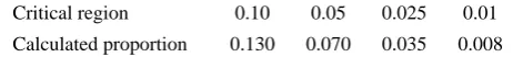
Table (1) summarises the results of the bootstrap study. The bottom row of the table gives the proportions of time that the calculated F-statistic fell beyond the critical values for different critical regions. This table presents relatively good evidence about the behaviour of the test. For the critical regions 0.10, 0.05 and 0.025 the calculated proportions are higher than the theoretical values, while we remember that we have rejected the assumption of no autocorrelation for the original data at the 0.10 level. The calculated proportion for the 0.01 is less than the theoretical value, which indicates that the test procedure will be conservative for the small critical regions.
Table 1. Simulation results of the first order autocorrelation test
Critical region 0.10 0.05 0.025 0.01
Calculated proportion 0.130 0.070 0.035 0.008
Table 2. Simulation results of the first order autocorrelation test using pelleted and grains diets data
Critical region 0.10 0.05 0.025 0.01
Calculated proportion 0.085 0.048 0.027 0.008
A second bootstrap study was conducted with a subset of eighteen groups of the digestibility data, which are pelleted and grains diets. The aim of the second study is to determine the effect of the small sample sizes
on the test procedure. While the other aspects of the bootstrap process were unchanged, we simulated 1000 data sets with a procedure exactly the same as before.
The results of the second study are summarised in Table (2). From this table we can see that, despite the possible rejection of the hypothesis of no autocorrelation for the original data at the level of 0.10, the calculated proportions are less than the theoretical values, which shows that for the small sample sizes the test procedure is conservative. Finally, while our simulation study is restricted to the first order autocorrelation, however, we could also extend our study to the higher orders and to see how the procedure works for small sample sizes.
Acknowledgements
I am indebted to the anonymous referee for a number of useful comments and suggestions, which help me to improve my paper.
References
1. Durbin, J. and Watson, G. S., Testing for serial correlation in least squares regression III. Biometrika, 58: 1-19 (1971).
2. Godfery, L., Testing for Multiplicative Heterosce-dasticity. J. Econometrics, 227-36 (1978).
3. Farebrother, R., The Durbin-Watson Test for Serial Correlation when there is no intercept in the Regression. Econometrica, 1553-63 (1980).
4. Engle, R. F., Wald, Likelihood-Ratio and Lagrangian Multiplier Tests in Econometrics. In: Z. Griliches and M. D. Intrilligator (Eds.), Annals of Econometrics, North- Holland, New York, (1984).
5. Fuller, W. A., Measurement Error Models. Wiley, New York, (1987).
6. Rasekh, A. R., Residuals in unequally replicated functional measurement error models. (Submitted to Communication is Statistics, Theory & Methods) (1998). 7. Fuller, W. A., Introduction to Statistical Time Series.
Wiley, New York, (1976).
8. Bishop, Y. M. M., Fienberg, S. E. and Holland, P. W., Discrete Multivariate Analysis: Theory and Practice. The MIT Press, (1975).