THE PERFORMANCE OF KARAFILLIS-BOYCE YIELD
FUNCTION ON DETERMINATION OF FORMING
LIMIT DIAGRAMS
M. Ganjiani and A. Assempour٭
Department of Mechanical Engineering, Sharif University of Technology Azadi Avenue P.O. Box 11365-9567, Tehran, Iran
*Corresponding Author
(Received: June 25, 2006 - Accepted in Revised Form: January 18, 2007)
Abstract Forming Limit Diagrams are useful tools for evaluation of formability in the sheet metals. In this paper the effects of yield criteria on predictions of the right and left-hand sides of forming limit diagrams (FLDs) are investigated. In prediction of FLD, Hosford 1979, “Karafillis-Boyce” (K-B) and BBC2000 anisotropy yield functions have been applied. Whereas the prediction of FLD is based on the “Marciniak and Kuczynski” model, thus a numerical approach using the Newton-Raphson method has been used. Forming Limit Diagrams have been obtained for Al 6111-T4 and AA5XXX alloys and results have been compared with published experimental data. Results indicate that predictions of FLD are very sensitive to selection of yield criterion. Also it was found that the FLD of K-B yield function has a better agreement than that by other yield criteria.
Keywords Marciniak and Kuczynski Model, Karafillis and Boyce, Hosford 1979, BBC2000, Yield Function, Newton-Raphson Method
ﻩﺪﻴﮑﭼ
ﻲﻨﺤﻨﻣ ﻞﻜﺷﺪﺣ ﻱﺎﻫ ﻞﻜﺷﻦﻴﻤﺨﺗ ﻱﺍﺮﺑ ﺪﻴﻔﻣﻱﺭﺍﺰﺑﺍ ﻲﻫﺩ
ﻕﺭﻭ ﻱﺮﻳﺬﭘ ﻲﻣﻱﺰﻠﻓ ﻱﺎﻫ
ﺪﻨﺷﺎﺑ . ﻦﻳﺍ ﺭﺩ
ﭗﭼ ﻭ ﺖﺳﺍﺭ ﺖﻤﺳ ﻪﺒﺳﺎﺤﻣ ﻱﻭﺭ ﻒﻠﺘﺨﻣ ﻢﻴﻠﺴﺗ ﻱﺎﻫﺭﺎﻴﻌﻣ ﺮﻴﺛﺎﺗ ﻪﻟﺎﻘﻣ ﻲﻨﺤﻨﻣ
ﻞﻜﺷ ﺪﺣ ﻱﺎﻫ ﻲﺳﺭﺮﺑ ﻲﻫﺩ
ﻲﻣ ﺩﻮﺷ . ﻲﻨﺤﻨﻣﻪﺒﺳﺎﺤﻣﺭﺩ ﻞﻜﺷﺪﺣﻱﺎﻫ
ﺩﺭﻮﻔﺳﺎﻫﻥﻮﭼﻱﺩﺮﮕﻧﺎﺴﻤﻫﺎﻧﻢﻴﻠﺴﺗﻱﺎﻫﺭﺎﻴﻌﻣ،ﻲﻫﺩ ۱۹۷۹
ﺲﻴﻠﻴﻓﺍﺭﺎﻛ،
-ﻲﺑﻭﺲﻳﻮﺑ ﻲﺑ
ﻲﺳ ۲۰۰۰ ﺖﺳﺍ ﻩﺪﺷﻝﺎﻤﻋﺍ .
ﻲﻨﺤﻨﻣﻥﺩﺭﻭﺁ ﺖﺳﺪﺑ ﻪﻛﺎﺠﻧﺁﺯﺍ ﻞﻜﺷﺪﺣ ﻱﺎﻫ
ﻝﺪﻣﻪﻳﺎﭘ ﺮﺑ ﻲﻫﺩ
ﻙﺎﻴﻨﻴﺷﺭﺎﻣ
-ﻲﻣﻲﻜﺴﻨﻳﺯﻮﻛ ﺭ ﻦﻳﺍﺮﺑﺎﻨﺑ ،ﺪﺷﺎﺑ
ﻦﺗﻮﻴﻧ ﻱﺩﺪﻋ ﺵﻭ
-ﺖﺳﺍ ﻩﺪﺷ ﻩﺩﺎﻔﺘﺳﺍ ﻥﻮﺴﻓﺍﺭ .
ﻲﻨﺤﻨﻣ ﺪﺣ ﻱﺎﻫ
ﻞﻜﺷ ﻱﺎﻫﮊﺎﻴﻟﺁﻱﺍﺮﺑﻲﻫﺩ
AA5XXX
ﻭ
Al 6111-T4
ﻩﺩﺍﺩﺎﺑﻥﺁﺞﻳﺎﺘﻧﻭﻪﺘﺸﮔﺝﺍﺮﺨﺘﺳﺍ ﻩﺪﺷﺮﺸﺘﻨﻣﻲﺑﺮﺠﺗﻱﺎﻫ
ﺖﺳﺍ ﻩﺪﺷ ﻪﺴﻳﺎﻘﻣ ﺕﻻﺎﻘﻣ ﻪﻴﻘﺑﺭﺩ .
ﻲﻣ ﻥﺎﺸﻧ ﺞﻳﺎﺘﻧﻦﻳﺍ ﻲﻨﺤﻨﻣ ﻪﻛﺪﻫﺩ
ﻞﻜﺷ ﺪﺣﻱﺎﻫ ﻊﺑﺎﺗﻉﻮﻧ ﺏﺎﺨﺘﻧﺍﻪﺑ ﻲﻫﺩ
ﺴﻫﺱﺎﺴﺣﻢﻴﻠﺴﺗ ﺪﻨﺘ
. ﻞﻜﺷﺪﺣﻲﻨﺤﻨﻣﻪﻛﻩﺪﺷﻩﺪﻫﺎﺸﻣﻦﻴﻨﭽﻤﻫ ﺲﻴﻠﻴﻓﺍﺭﺎﻛﻢﻴﻠﺴﺗﻊﺑﺎﺗﺯﺍﻪﺠﺘﻨﻣﻲﻫﺩ
-ﺲﻳﻮﺑ
ﺩﺭﺍﺩﻢﻴﻠﺴﺗﻊﺑﺍﻮﺗﻪﻴﻘﺑﻪﺑﺖﺒﺴﻧﻲﺑﺮﺠﺗﺞﻳﺎﺘﻧﺎﺑﻱﺮﺘﻬﺑﻖﺑﺎﻄﺗ .
1. INTRODUCTION
In sheet metal operation, the amount of deformation is restricted by the occurrence of localized necking. Experimental investigations revealed that localized necking of sheet metals could be well described by a diagram in principal strain plane, namely Forming limit diagram (FLD). Thus the FLD is convenient tool to be used as the reference in evaluation of the formability in sheet metals.
Keeler and Backofen [1] and Goodwin [2]
Van Minh, et al. [6], Yamaguchi and Mellor [7], Tadros and Mellor [8] examined the effects of different types of initial non-uniformity on FLD. Barata da Rocha et al. [9] used the M–K method to predict FLD. They also used Hill’s 1948 yield criterion and analyzed the influence of the directional r-values. Kuroda and Tvergaard [10] investigated the influence of different orthotropic yield criteria in the M–K model and showed that disorientations of the orthotropic axes inside and outside the necking band can lead to significant differences in FLD prediction. Cao et al. [11] predicted localized thinning of sheet metal alloys for linear and nonlinear strain paths in the Marciniak-Kuczynski (M-K) model. Kuroda and Tvergaard [12] studied the influence of the yield criterion on Forming Limit Diagram by using the M-K model. Butuc et al. [13] used the M–K model
and proposed a solution scheme based on a Newton–Raphson solver in order to determine the unknown parameters in the M–K model. Banabic et al. [14] compared different modeling approaches to predict the forming limit diagram (a finite element based approach, the M–K model, the Hora et al., Swift’s diffuse and Hill’s localized necking
approach) using an orthotropic yield criterion BBC2003. They showed that the results of the M– K model and the finite element based approach are very close to each other and agreed very well with the experimental necking FLD.
A thorough review of the effects of yield surface shape on the prediction of FLDs was offered by Barlat [22]. In his work, several important characteristics of the yield surface are identified and a parameter is introduced that quantifies some of the differences between various yield criteria. This parameter, P, defined as the
ratio of the yield stress in plane strain to that in balanced-biaxial tension has been shown to correlate well with predictions of limit strains based on the M-K analysis.
The purpose of this paper is to investigate the effect of three yield surface shape namely Hosford 1979, “Karafillis - Boyce” (K-B) and BBC2000 on prediction of the right and left hand sides of Forming Limit Diagrams. Thus a developed numerical method on M-K model for prediction of the FLD is applied. The numerical approach is based on the Newton-Raphson method. For calculating FLD, two hardening laws such as
Power law and Voce hardening laws [15] are employed. Also, the predicted FLD is compared with the experimental data for Al 6111-T4 and AA5XXX metals.
2. YIELD CRITERIA
While there exists numerous yield criteria that incorporate the effects of plastic anisotropy, we examine the effects of three specific criteria in order to find a general rule for making judgment on the effects of plastic anisotropy on forming limit. The first of these is Hosford 1979’s yield criterion:
a y σ ) 1 R ( a ) 2 σ 1 σ ( R a 2 σ a 1
σ + + − = + (1)
where σ1 and σ2 are the in-plane principal stresses and σy is the equivalent stress, in this case, equal to the yield stress in uniaxial tension. The coefficient R is normal anisotropy and is defined
by:
) 90 R 45 R 2 0 R ( 4 1
R= + + (2)
where R0, R45 and R90 are the ratios of transverse to
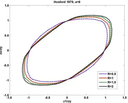
through-thickness strains under uniaxial tension at 0, 45° and 90° to the rolling direction. This criterion is based on upper-bound crystallographic calculations. The suggested exponent, a, is 6 for
BCC materials and 8 for FCC materials. This criterion has been plotted for both cases for various values of R in Figures 1 and 2, respectively. As
shown in the figures, the yield surfaces are quite flat and the positions of plane strain relative to that of balanced-biaxial stretching are quite insensitive to the value of R.
The second yield surface of the anisotropic material with orthotropic symmetry is described by a non-quadratic yield criterion developed by “Karafillis and Boyce” [15]. The K-B yield criterion was constructed by mixing two yield functions, Ψ1 and Ψ2. As shown in Equations 3-5,
Figure 1. Hosford's yield criterion with an exponent of 6 for various values of R.
Figure 2. Hosford's yield criterion with an exponent of 8 for various values of R.
upper bound as a changes from 2 to ∞.
a 1 2 2 Ψ C 1 Ψ ) C 1 ( y σ ⎥ ⎥ ⎦ ⎤ ⎢ ⎢ ⎣ ⎡ − +
= (3)
where, a 2 S 1 S a 3 S 1 S a 3 S 2 S 1
Ψ = − + − + − (4)
a 3 S a 2 S a 1 S ( 1 1 a 2 a 3 2
Ψ + +
+ −
= (5)
a and c are material constants and Si is the principal values of the isotropic plasticity equivalent stress tensor and σy is the average yield
stress in uniaxial tension obtained experimentally. A fourth order tensorial operator, L, introduces the
material anisotropy, i.e.
σ : L
S= (6)
Where s is isotropic plasticity stress tensor, σ is the Cauchy stress in the anisotropic material:
] 12 σ 23 σ 31 σ 33 σ 22 σ 11 σ [
σ= (7)
and L is a fully symmetric and traceless fourth
order tensor: ⎥ ⎥ ⎥ ⎥ ⎥ ⎥ ⎥ ⎥ ⎦ ⎤ ⎢ ⎢ ⎢ ⎢ ⎢ ⎢ ⎢ ⎢ ⎣ ⎡ + − − − + − − − + = 6 C 0 0 0 0 0 0 5 C 0 0 0 0 0 0 4 C 0 0 0 0 0 0 3 / ) 2 C 1 C ( 3 / 1 C 3 / 2 C 0 0 0 3 / 1 C 3 / ) 1 C 3 C ( 3 / 3 C 0 0 0 3 / 2 C 3 / 3 C 3 / ) 3 C 2 C ( L (8) Where c1, c2, …, c6 are material constants. The last
criterion is BBC2000 yield criterion. This yield function is a new yield criterion for orthotropic sheet metals under plane stress conditions. It is derived for the one proposed by Barlat and Lian in 1989 [22]. Two additional coefficients, namely b and c, have been introduced in order to allow a better representation of the orthotropic sheet metals plastic behavior. The equivalent stress is defined by the following relationship:
K 2 1 K 2 ) Ψ c 2 ( ) a 1 ( K 2 ) Ψ c Γ b ( a K 2 ) Ψ c Γ b ( a σ ⎥ ⎥ ⎦ ⎤ ⎢ ⎢ ⎣ ⎡ − + − + +
= (9)
Where a,b,c and K are material parameters,
described in Equation 8. Hence, in the reference system associated to the directions of plastic orthotropy, the tensor L has six non-zero
components for 3D conditions and four components for a plane stress state. Let (x, y, z) be
the reference frame associated to the directions of plastic orthotropy. For a rolled sheet, x, y, and z
represent the rolling direction, the transverse direction, and the perpendicular to the plane of the sheet metal, respectively. The components of the s tensor can be expressed as follows in this frame: 0 13 S 31 S , 0 32 S 23 S , 21 σ g 21 S , 12 σ g 12 S , 22 σ ) f (e , 11 σ ) e d ( 33 S , 22 σ f 22 σ e 22 S , 11 σ e 11 σ d 11 S = = = = = = + − + − = + = + = (10)
Where d, e, f and g, the four independent
components of the tensor L, are anisotropy
coefficients of material. The second and third invariants of the deviatoric tensor s have the following expressions: kk S ) ij S t e d ( 3 J , ij S t e d 2 kk S 2
J = − =− (11)
where the Greek indices take the values 1 and 2.
ij S t e d 3 I , kk S 2
I = = (12)
The quantities are not affected by the rotations that leave unchanged the third axis (ND). Thus, in the case of the plane stress of sheet metals, we can use
I2and I3 instead of J2 and J3 in order to define the functions Γ and Ψ. We have adopted the following expressions for these functions:
2 1 3 I 2 2 2 I Ψ , 2 I Γ ⎥ ⎥ ⎥ ⎦ ⎤ ⎢ ⎢ ⎢ ⎣ ⎡ − ⎟ ⎟ ⎠ ⎞ ⎜ ⎜ ⎝ ⎛ = = (13)
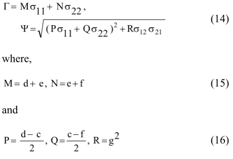
By using Equations 11-13, we can express Γ and Ψ as explicit dependences of the actual stress components; 21 12 2 R ) 22 Q 11 P ( , 22 N 11 M σ σ + σ + σ = Ψ σ + σ = Γ (14) where, f e N , e d
M= + = + (15)
and 2 g R , 2 f c Q , 2 c d
P= − = − = (16)
The K value is set in accordance with the
crystallographic structure of the material: K = 3 for
BCC alloys, and K = 3 for FCC alloys.
These criteria have been plotted for AA5XXX in Figure 3. Material constants of this metal for these yield criteria are listed in Tables 1 and 3. As shown in Figure 3, at the position balanced - biaxial stretching, the Hosford’s yield surface is coincided to the BBC2000’s yield surface. At other positions, the differences between these two yield function is negligible. But the differences between Karafillis - Boyce yield surface and other two yield surfaces are sensible.
3. REVIEW OF MARCINIAK AND KUCZYNSKI MODEL
Figure 3. Comparison of different yield surfaces.
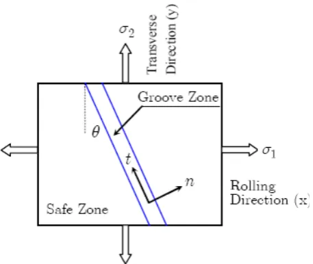
Figure 4. Assumption of a narrow groove in the sheet surface for prediction of FLD in the M - K model.
follows:
b nn F a nn F
b nt F a nt F
= =
(17)
where Fnn and Fnt are forces in the normal and
tangential directions in the groove. By introducing the stress state in these areas, Equation 17 could be
rewritten as follows:
b 0 t ) b 3 ε ( p x e b nn σ a 0 t ) a 3 ε ( p x e a nn σ
b 0 t ) b 3 ε ( p x e b nt σ a 0 t ) a 3 ε ( p x e a nt σ
= =
(18)
where σnn and σnt are stress components in the “n” and “t” directions, ta0 and tb0 are initial thicknesses in the safe and groove regions, respectively. Non-uniformity factor, f, can be
expressed as a function of the initial defect: )
a 3 ε -b 3 ε ( p x e f
f= 0 (19)
Herein f0 is the initial non-uniformity factor and
denotes by tb0/ta0, and ε3 is the strain in thickness direction calculated by incompressibility condition:
) 2 ε 1 ε ( 3
ε =− + (20)
Thus, force equilibrium conditions are summarized as:
a nt σ b nt σ f
b nn σ b nn σ f
= =
(21)
It is assumed that the strain increments parallel to the groove are the same in both regions (compatibility condition):
a tt ε d b tt ε
d = (22)
By using the force equilibrium and compatibility conditions, the unknown parameters are obtained. The unknown parameters are including stress and strain components, whereas, using flow rule, the strain components are related to effective strain and stress state:
ij y ε d ij ε d
σ ∂
σ ∂
= (23)
TABLE 1. Material Constants Describing the K - B Yield Function [18].
c6 c3 c2 c1 c a Metal
0.48 0.96 1.08 1.03 0.63 26 Al 6111-T4
0.99 1.07 0.80 1.05 0.63 26 AA5XXX
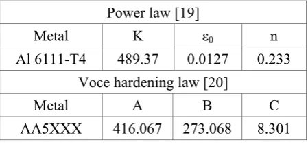
TABLE 2. Material Constants Describing the Hardening Laws.
Power law [19]
n
ε0 K
Metal
0.233 0.0127
489.37 Al 6111-T4
Voce hardening law [20]
C B
A Metal
8.301 273.068
416.067 AA5XXX
TABLE 3. Mechanical Constants Describing BBC2000 and Hosford Yield Functions for AA5XXX.
R K Q P N M c b a
0.63 4 -0.725 0.726 0.504 0.507 0.730 0.982 0.663
4. COMPUTATION PROCESS
To calculate the limit strains, the safe region is loaded, i.e. it is assumed the safe region is stretched with constant stress relation α. For this purpose, a value for α, between 0 and 1 is selected and note that this value must remain constant at entire time during the process. At starting, a small value for effective strain increment dεa (for example 0.0001) is assumed. Substituting εa in the hardening law, the effective stress σY is obtained. Since the effective stresses by hardening law and yield function are equal, thus a
x
σ and a y
σ can be obtained. A relationship between effective strain
and effective stress can be represented by the so - called Power law:
n ) 0 ( K
Y= ε +ε
σ (24)
where, K is the strength coefficient, ε0 is the pre-strain and n is the hardening law exponent. Also Voce [15] hardening law has been used to describe behavior of aluminum alloys that are insensitive to the strain-rate sensitively:
) C ( p x e B A
Y= − − ε
σ (25)
Where A, B and C are material constants. Using the
assumed dεa, stress components and flow rule, strain components dεax and dεay are calculated. Since the groove has an angle with respect to transverse direction, it is required to find stress and strain states in the groove direction. This work is needed for satisfying the compatibility and force equilibrium conditions. Using the rotation matrix, the vectors for strain and stress tensors are changed to the groove system of coordinates:
⎥ ⎥ ⎦ ⎤ ⎢
⎢ ⎣ ⎡
σ σ
σ σ = σ
= σ
tt nt
nt nn T T xyz T
ntz (26)
with,
⎥ ⎦ ⎤ ⎢
⎣ ⎡
θ θ
−
θ θ
=
) ( COS ) ( Sin
) ( Sin ) ( COS
T (27)
where T is the rotation matrix and TT is transpose of rotation matrix. In this paper, for calculating the unknown parameters at groove region, the Newton-Raphson method is applied. Consider N functional Fi relations to be zeroed involving
variables x1, i=1,2,...,N. as follows:
. N , ... , 2 , 1 i 0
) N x , ... , 2 x , 1 x ( i F
= =
(28)
Using Taylor series, functions Fi can be expanded
as follows:
) 2 x ( O j x N
1 j xj
i F )
x ( i F ) x x ( i
F ∑ δ + δ
= ∂ ∂ + = δ
In matrix notation, Equation 29 is reduced to: ) 2 x δ ( O x δ . J ) x ( F ) x δ x (
F + = + + (30)
Where J is the matrix of partial derivatives and is called the Jacobian matrix.
j x i F ij J ∂ ∂
= (31)
By neglecting terms of order δx2 and higher and by setting F(x+δx)=0, we obtain a set of nonlinear equations:
0 F x .
J δ + = (32)
or,
F . J x =− −1
δ (33)
Then, the variable δx is added to the solution
vector:
x old x new
x = +λδ (34)
where λ is the Newton step length. Using a backtracking algorithm, an acceptable λ can be found. The following steps must be considered as the simplest backtracking line search to find λ:
Step 1. Set
λ = 1.Step 2. While:
4 10 ) old x new x ( . ) x ( g ) old x ( g ) new x (
g > +∇ − (35)
set λ =λs.
Step 3. Set
λK= λ.Equation 35 is suggested by Armijo [19] as the condition for finding the optimum λ. In this equation g(x) is defined as;
F . F ) x (
g = (36)
Typically, s = 0.8 or 0.5, meaning that based on the
linear extrapolation, a small decrease in g(x) is accepted. To exit the Newton’s calculation loops, it is required to define a criterion. In the present formulations, there exists a vector of function which has four components. All components of this vector have the same important rank. Thus, the maximum value among these components has been selected to be compared with the tolerance in the Newton’s loop. i.e.:
i F 4 1 i max F = =
∞ (37)
This is called ∞ - norm. Since the unknown parameters in this region are including,
b nt σ , b tt σ , b nn
σ and dεb, the vector of values x is defined as: T b d b nt σ b tt σ b nn σ
x=⎢⎣⎡ ε ⎥⎦⎤ (38)
Using the compatibility and force equilibrium conditions, three equations for the vector of functions are obtaining. In this paper, the energy relation is used as the 4th equation:
Y σ b ε d b nt σ b nt ε d b tt σ b tt ε d b nn σ b nn ε
d + + = (39)
Thus, vector of functions, F is introduced as follows: T 4 F 3 F 2 F 1 F
F=⎢⎣⎡ ⎥⎦⎤ (40)
where, 0 1 Y σ b ε d b nt σ b nt ε d b tt σ b tt ε d b nn σ b nn ε d 1
F = + + − = (41)
0 1 a tt ε d b tt ε d 2
F = − = (42)
0 1 a nn σ b nn σ f 3
0 1 b nt σ b nt σ f 4
F = − = (44)
and the Jacobian matrix is written as:
⎥ ⎥ ⎥ ⎥ ⎥ ⎥ ⎥ ⎥ ⎥ ⎥ ⎥ ⎥ ⎥ ⎦ ⎤ ⎢ ⎢ ⎢ ⎢ ⎢ ⎢ ⎢ ⎢ ⎢ ⎢ ⎢ ⎢ ⎢ ⎣ ⎡ ∂ ∂ ∂ ∂ ∂ ∂ ∂ ∂ ∂ ∂ ∂ ∂ ∂ ∂ ∂ ∂ ∂ ∂ ∂ ∂ ∂ ∂ ∂ ∂ ∂ ∂ ∂ ∂ = b ε d 4 F b nt σ 4 F b tt σ 4 F b nn σ 4 F b ε d 3 F b nt σ 3 F b tt σ 3 F b nn σ 3 F b ε d 2 F b nt σ 2 F b tt σ 2 F b nn σ 2 F b ε d 1 F b nt σ 1 F b tt σ 1 F b nn σ 1 F
J (45)
Calculating of limiting strains is repeated for different value of θ between 0 and 90°. It is important to note that considering of groove orientation is necessary for calculating the limit strain especially for the left hand side of FLD. Changing in the groove orientation is obtained using definition of the natural strain as follow:
0 l 1 l ln ε
d = (46)
where l0 and l1 are initial and deformed lengths,
respectively. Using Equation 46 and considering Figure 5, strain increments in the rolling and transverse directions are obtained as follows:
) 1 ε d ( exp ln 1 ε
d a a
a
a′⇒ ′=
= (47)
) 2 ε d ( exp ln 2 ε
d b b
b
b′⇒ ′=
= (48)
Using Equations 47 and 48 and definition of tangent of an angle, we have:
) 2 ε d 1 ε d ( exp ) 0 θ ( tg ) 2 ε d 1 ε d ( exp ) θ (
tg = − = −
′ ′ = b a b a (49) Minimum value of major localization strain is
selected among the calculation loops by variation
of θ. The selected minimum strain for any value of
α is used in plotting of the FLD. This progression is shown in appendix I as a flowchart.
5. RESULTS AND DISCUSSIONS
In this paper, the effects of the preceding yield functions on prediction of the FLD have been studied in Al 6111-T4 and AA5XXX metals. Mechanical properties of these metals are listed in Table 1.
To calculate the limit strains, Power law relationship is selected for Al 6111-T4 and Voce hardening law is chosen for AA5XXX. Table 2 shows material constants related to these hardening laws.
Figure 6 compares the calculated FLD in AA5XXX with experimental data. To calculate the limit strains (Forming Limit Diagram) of AA5XXX f0 is selected 0.9960. As shown in
Figure 6, the predicted FLD has good agreement with the experimental data. To validate the FLD of K-B yield function, the predicted FLD is compared with BBC2000 [22] and Hosford [23] yield functions. The mechanical constants related to these two yield functions for AA5XXX alloy are listed in Table 1.
In Figure 7, the predicted FLD by applying the K-B yield function is compared with the FLD of Hosford and BBC2000 yield functions. The FLD of BBC2000 and Hosford yield criteria has been also calculated by similar method in this paper. It is observed from Figure 7 that the FLD by K - B yield function is safer than the FLD by BBC2000 and Hosford yield functions with the exponent a =
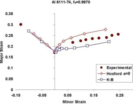
8. To calculate the FLD of Al 6111-T4, the non-uniformity factor, f0, is selected 0.9970. For this
metal, the Power law is selected to describe the relation between effective strain and effective stress. R is necessary property for describing
Hosford yield function in Al 6111-T4 which is 0.63. The exponent in the Hosford relationship, a,
is selected 8. Figure 8 shows comparison of predicted FLD using “Karafillis - Boyce” and “Hosford” yield functions. The predicted FLD by K-B yield function has better agreement than that by Hosford yield criterion.
Figure 5. Groove orientation in the M - K model.
Figure 6. Comparison of Predicted FLD using K - B yield criterion and experimental data [20].
Figure 7. Comparison of FLD of different yield criteria with the experimental results [20].
Figure 8. Comparison of Predicted FLD using K - B and
Hosford yield functions and experimental data [19]. with other experimental data. Figure 9 and Figure
10 reveal the result of this comparison. As shown in all above figures, the left hand side (LHS) of FLD is linear and it is not dependent to the selection of yield function.
6. CONCLUSION
In this paper, to calculate the limit strains, the “Marciniak and Kuczynski” (M-K) model has been
Figure 9. Comparison of FLD by K - B and Hosford yield criteria and experimental results [24].
Figure 10. Comparison the right - hand side of FLD by K – B and Hosford yield criteria and experimental results [21].
has linear variation from FLD0.
7. NOMENCLATURE
σ1,σ2 Principal stress components.
σnn,σtt,σnt Stress components in the groove coordinate.
Y
σ Effective stress obtained by hardening law.
y
σ Effective stress obtained by yield function.
ε0, K, n, m, A, B, C Material constants describing
hardening laws.
a, c, c1, …, c6 Material constants describing
K - B yield function.
c , b ,
a , M,N,P,Q,R Material constants describing
BBC2000 yield function.
R Normal anisotropy.
ε Effective plastic strain. ε& Rate of effective plastic strain.
ε
d Effective plastic strain
increment. nt
dε , tt dε , nn
dε Strain increments in the groove coordinate.
3 dε , 2 dε , 1
dε Strain increments in the
material coordinate.
a Ratio of stresses along the
strain path.
T Rotation matrix.
dλ Plastic multiplier.
Fnn, Fnt Force equations in the groove directions.
f Non-uniformity factor.
δx Newton’s step.
J Jacobian matrix.
θ Angle between the groove
coordinates and the material coordinates.
λ Newton step length.
8. REFERENCES
1. Keeler, S. P. and Backofen, W. A., “Plastic Instability and Fracture in Sheets Stretched Over Rigid Punches”,
Transactions of The ASM, 56, (1963), 25-48.
2. Goodwin, G. M., “Application of Strain Analysis to Sheet Metal Forming Problems in the Press Shop", Society of Automotive Engineers, Technical Paper No., (1968), 680093.
3. Keeler, S. P., “Determination of Forming Limits in Automotive Stampings”, Society of Automotive Engineers, Technical paper No., (1965), 650535.
4. Marciniak, M. and Kuczynski, K., “Limit Strains in the Processes of Stretch - Forming Sheet Metals”, Int. J.
Mech. Sci., 9, (1967), 609–20.
APPENDIX I. The Progression Flowchart for Prediction of FLD.
Int. J. Mech. Sci., (1973), 15: 789-805.
6. Van Minh, H., Sowerby, R. and Duncan, J. L., “Probabilistic Model of Limit Strains in Sheet Metal”,
Int. J. Mech. Sci., 17, (1975), pp. 339-349.
Stretching”, Int. J. Mech. Sci., 18, (1976), 85-93.
8. Tadros, A. K. and Mellor, P. B., “Some Comments on the Limit Strains in Sheet Metal Stretching”, Int. J.
Mech. Sci., 17, (1975), pp. 203-208.
9. Barata da Rocha, F. B. and Jalinier, J. M., “Prediction of the Forming Limit Diagrams of Anisotropic Sheets in Linear and Non - Linear Loading”, Mater. Sci. Eng.,
68, (1984–1985), 151–64.
10. Kuroda, Mand. and Tvergaard, V., “Forming Limit Diagrams for Anisotropic Metal Sheets with Different Yield Criteria”, Int. J. Solids Struct., 37, (2000), 5037–59.
11. Cao, J., Yao, H., Karafillis, A. and Boyce, Mary C., “Prediction of Localized Thinning in Sheet Metal Using a General Anisotropic Yield Criterion”, Int. J. of
Plasticity, 16, (2000), 1105-1129.
12. Kuroda, Mits. and Tvergaard, V., “Forming Limit Diagrams for Anisotropic Metal Sheets with Different yield criteria”, Int. J. of Solids and Struct., 37, (2000),
5037-5059.
13. Butuc, M. C., Barata da Rocha, A., Gracio, J. J. and Ferreira Duarte, J., “A more general model for forming limit diagrams prediction” J. Mater. Process. Technol.,
(2002), 125–126, 213–18.
14. Banabic, D., Aretz, H., Paraianu, L. and Jurco, P., “Application of Various FLD Modeling Approaches”, Modeling Simul. Mater. Sci. Eng., 13, (2005), 759–769. 15. Voce, E., “The Relationship Between Stress and Strain
for Homogeneous Deformation”, J. Inst. Met., 74,
(1948), 537–540.
16. Armijo, L., “Minimization of Functions Having Lipschitz Continuous First Partial Derivatives”, Pacific
J. Math., (1966), 6:1-3.
17. Karafillis, A. P. and Boyce, M. C., “A General
Anisotropic Yield Criterion Using Bounds and Transformation Weighting Tensor”, J. Mech. Phys.
Solids, 41, (1993), 1859.
18. Yao, H. and Cao, J., “Prediction of Forming Limit Curves Using an Anisotropic Yield Function with Prestrain Induced Back Stress”, Int. J. Plasticity, 18,
(2002), 1013-1038.
19. Chow, C. L. and Yang, X – J., “Prediction of the Forming Limit Diagram on the Basis of the Damage Criterion under Non - Proportional Loading”, Proceed.
Instit. Mech. Eng., 4: ProQuest Science Journals,
(2001), 215.
20. Butuc, M. C., Banabic, D., Barata da Rocha, A., Gracio, J. J., Ferreira Duarte, J., Jurco, P. and Comsa, D. S., “The Performance of Yld96 and BBC2000 Yield Functions in Forming Limit Prediction”, J. of Mater.
Process. Tech., (2002), 125-126, 281-286.
21. Siguang, Xu, and Weinmann, Klaus J., “Prediction of Forming Limit Curves of Sheet Metals Using Hill’s 1993 User - Friendly Yield Criterion of Anisotropic Materials”, Int. J. Mech. Sci., (1998), 40, 913-925.
22. Barlat, F. and Lian, J., “Plastic Behavior and Stretchability of Sheet Metals. Part I: A Yield Function for Orthotropic Sheet Under Plane Stress Conditions”,
Int. J. Plasticity, (1989), 5, 51-56.
23. Hosford, W. F., “On Yield Loci of Anisotropic Cubic Metals”, 7th North American Metalworking Research
Conference Proceedings, SME Dearborn, Michigan,
(1979), 191.
24. Wu, P. D., Graf, A., MacEwen, S. R., Lloyd, D. J., Jain, M. and Neale, K. W., “On Forming Limit Stress Diagram Analysis”, Int. J. Solids and Struc., (2005),
![Figure 9. Comparison of FLD by K - B and Hosford yield criteria and experimental results [24]](https://thumb-us.123doks.com/thumbv2/123dok_us/242458.2018946/10.595.57.539.71.731/figure-comparison-fld-hosford-yield-criteria-experimental-results.webp)