Designing different Sampling Plans Based on Process Capability Index

Please cite this article as: M S. Fallah Nezhad, S. Seifi, Designing Different Sampling Plans Based on Process Capability Index, International Journal of Engineering (IJE), TRANSACTIONSB: Applications Vol. 29, No. 8, (August 2016) 1120-1130

International Journal of Engineering

J o u r n a l H o m e p a g e : w w w . i j e . i r

Designing Different Sampling Plans Based on Process Capability Index

M. S. Fallah Nezhad*, S. Seifi

Faculty of Industrial Engineering, Yazd University, Yazd, Iran

P A P E R I N F O

Paper history: Received 31 October 2015

Received in revised form 08 June 2016 Accepted 14 July 2016

Keywords:

Process Capability Index

Repetitive Group Sampling Plan (RGS) Acceptance Sampling Plan

Average Sample Number (ASN) Multiple Dependent State (MDS) Sampling Plan

Double Sampling Plan

A B S T R A C T

Acceptance sampling models have been widely applied in companies for evaluation the raw material as well as the final products. Meanwhile, process capability indices (PCIs) have been used in various industrial environments as capability measures that are obtained based on process departure from a target, process yield, process consistency and process loss. In this research, first a repetitive group sampling (RGS) plan based on process capability index is developed for variables inspection. Then the optimal parameters of proposed RGS plan are determined and also a new multiple dependent state (MDS) sampling plan, a double sampling plan (DSP) and a sampling plan for resubmitted lots are developed and finally, a comparison study is carried out between the proposed sampling plans and the results are elaborated.

doi: 10.5829/idosi.ije.2016.29.08b.12

1. INTRODUCTION1

Because of the competition between suppliers and its importance, producing a product with good quality is a basic need of any production process. We can increase product quality and reduce waste using statistical techniques. This action can bring customer satisfaction and reduce costs and finally increase sales in market. To produce a product with high quality, it is needed to control and measure the quality of products at all steps of processes. A set of these measurements is defined as process capability analysis. One application of the process capability analysis is to make decision about the acceptance of a lot received from supplier in any industrial environment. Lot acceptance sampling plans provide a method for evaluating the quality of a received lot based on an inspected sample. These sampling plans are used by suppliers, manufacturers, contractors and service providers in a wide range of industrial environments. These plans are applied as a

1_{*Corresponding Author’s Email: [email protected] (M. S.}

Fallah Nezhad)

method of quality assurance that reduce the risk of both producers and consumers.

Among the classical methods of acceptance sampling plan, variable sampling plan is applied for quantitative analysis of quality characteristics. Although the use of variable sampling plans is more difficult compared to attribute sampling plan, but it is less risky and has less sample size.

Variable sampling plans are designed for quality characteristics that follow specified probability distribution function in continues scale. One of assumptions of variable sampling plan is the normality of quality characteristics. Process capability index is a continuous variable with a known probability distribution that is used for analyzing the production process thus it can be used for designing sampling plans.

Sampling plan has been widely discussed in the previous decades. The basic concepts of variables sampling plans were presented by Jennett and Welch [1] and Moskowitz and Tang [2]. Pearn and Wu [3] designed a variable sampling plan for very low fraction of defectives. Wu [4] proposed a method for estimating process capability under Bayesian approach based on subsamples collected over time from an in-control process. A new system of skip-lot sampling plan defined as SkSP-R was proposed by Balamurali et al. [5] that is efficient to minimize the cost of the lot inspection. A sampling plan based on process capability index was developed by Wu et al. [6] for the situation where resampling is permitted on lots which are not accepted on the main inspection. Suresh and Sangeetha [7] introduced an acceptance sampling plan for construction of Bayesian chain sampling plan (BChSP-1) using quality regions. A double sampling plan (DSP) based on truncated life tests in Rayleigh distribution was proposed by Aslam [8].

Sherman [9] presented a new acceptance sampling plan for the inspection of attributes quality characteristics known as the repetitive group sampling (RGS) plan. In the past years a repetitive mixed sampling plan based on the process capability index was developed by Aslam et al. [10]. Wu et al. [11] proposed a RGS plan based on variables inspection. Also three types of RGSs using the generalized process capability index of multiple characteristics were investigated by Aslam et al. [12]. In another work, Aslam et al. [13] developed a variable RGS plan by considering process loss. Suresh et al. [14] proposed a Bayesian repetitive deferred sampling plan indexed through relative slopes. A multiple deferred state sampling inspection (MDS sampling plan) was presented by Wortham and Baker [15]. Soundararajan and Vijayaraghavan [16] proposed a method for designing multiple dependent (deferred) state sampling plans. Also Vaerst [17] designed a procedure to construct multiple deferred state sampling plan. Aslam et al. [18] extended the idea of MDS sampling plans based on process capability index when the quality characteristic of the product follows the normal distribution.

In addition, a new acceptance sampling plan for resubmitted lots was investigated by Govindaraju and Ganesalingam [19]. A variable sampling plan for resubmitted lots based on process capability index was developed by Aslam et al. [20] for normally distributed processes. Also Balamurali et al. [21] proposed a variable RGS plan for minimizing ASN. Balamurali and Jun [22] proposed a RGS procedure for variable sampling plans. An optimal double-sampling plan based on process capability index was proposed by Fallah Nezhad and Seifi [23] in order to reduce the average sample number. Balamurali and Subramani [24] proposed the procedures for designing variables RGS

plan indexed by indifference quality level and the relative slope on the operating characteristic curve.

In this research, first we propose a variable RGS plan based on process capability index Cpm. Then the optimal parameters of developed RGS plan are obtained with considering the constraints related to the risk of consumer and producer. Also we present various variable sampling plans based on process capability index Cpm_{, then a comparison study is done between the}

developed sampling plans based on ASN criterion and the results are analyzed.

This research is organized as following. In section 2 the exact probability distribution function of process capability index is introduced. In section 3 a brief introduction of RGS, DSP, MDS and sampling plan for resubmitted lots are presented. A simulation study is presented in section 4. Finally, the results of comparison study and conclusions are presented in section 5 and section 6, respectively.

The main contributions of this research are as follows: Developing a RGS plan based on exact probability distribution function of Cpm_.

Comparing the performance of different proposed sampling plans.

2. THE EXACT PROBABILITY DISTRIBUTION FUNCTION OF PROCESS CAPABILITY INDEX

The formula for evaluating process capability index is defined as follows:

( 1 )

, 6 USL LSL

C_pm __

where   E X( T)2 and USL LSL, _{are upper and}

lower specification limits and

T

is the target value presented by customers or product designer. The parameter of  2

is usually unknown and have to be estimated; one estimation is as follows (Chan et al. [25]):

( 2 )

2

( )

ˆ ,

1 1

n X_i T

n i

  

 

The resultant estimator is obtained as follows:

( 3 )

( )

ˆ _,

ˆ 6 USL LSL

C_pm _

Since the process measurement arises from a normal distribution, thus the probability Pr(Cˆpmk C0)is

obtained as follows (Chan et al. [25]):

( 4 )

2 ₁

2 2

ˆ 2

Pr( ) exp dw,

2 _{1 0}

! 2

j _a

n j

C _w

C_pm C e w

n

j j j



      

    

  _  _{ }     _{ }

where aCpm2 (1/ )(n n1) and   2 2

/

n T

   _. Therefore, the statistical properties of process capability index Cˆpm can be analyzed for the general cases and we

can use this probability function for evaluating process capability index in sampling plans.

3. PROPOSED PLANS

3. 1. Proposed Variables RGS Plan Variables RGS plan is one of the effective sampling plans and the parameters in the proposed sampling plan are as follows:

sample size

n

1=the lower threshold of process capability index for rejecting the lot based on the single sample

k

2=the upper threshold of process capability index for

accepting the lot based on the single sample

k

Now we explain procedure of proposed plan with the real example. In many industries, the process capability of systems, materials, and products needs to be compatible with the specified engineering tolerances. In practical case, we consider a company that produce machine tools. This company needs to keep actual production (which includes machine tools) within the desired tolerances. The company engineers define a dimensional tolerance for each portion of tool and estimate process capability index for them. Finally, their decision making about received lot based on the process capability index and RGS procedure will be as follows: Step 1: Collect a sample with n observation.

Step 2: Accept the lot if 2

ˆ pm

C k _{and reject the lot if}

1

ˆ

pm

C k _where k₂k_{1. If} 1 2

ˆ pm

k C k _{, so repeat steps 1}

and 2.

The OC function of the RGS plan, which includes the proportion of lots that are expected to be accepted for given product quality, (a) is as follows:

( 5 ) ( ) Pa ,

P C_{a pm} P_r P_a

 

OC function can be rewritten as follows:

( 6 ) ˆ Pr( ) 2

( ) _{ˆ ˆ} ,

1 Pr( ) Pr( )

1 2

C k

P_a pm

P C_{a pm}

P_r P_a C_pm k C_pm k



 

    

Therefore, based on the plan of Balamurali and Jun [22], and considering the producer risk,  and consumer risk, , model constraints depending on the different values of CAQL,CLTPD can be defined as follows:

( 7 ) ˆ Pr( ) 2

a = a_{1 ˆ ˆ} 1 ,

1 Pr( ) Pr( )

1 2

C_pm k

C_pm C_AQL

C_pm k C_pm k 

          and: ( 8 ) ˆ Pr( ) 2

a = a ,

2 1 Pr(ˆ ) Pr(ˆ )

1 2

C_pm k

C C

pm LTPD _{C k C k}

pm pm





   

   

where a1CAQL2 (1/ )(n n1),

2

2 LTPD(1 / )( 1)

a C  n n _.

Also in the first constraint, 2

ˆ

Pr(C_pmk ) _and

1

ˆ Pr(C_pm k ) are the probabilities of accepting and rejecting the lot at AQL point based on single sample. In addition, in

second constraint, 2

ˆ

Pr(C_pmk ) _and

1

ˆ

Pr(Cpmk ) are the probabilities of accepting and rejecting the lot at LQL point based on single sample.



is producer risk and  is consumer risk, CAQLisdefined as the value of process

capability index in the quality level of AQL and CLTPDis

defined as the value of process capability index in the quality level of LTPD.

The objective function of model is to minimize the ASN and the number of sampling steps is equal

to 1 2

1

ˆ ˆ

Pr(Cpm k ) Pr(Cpm k )

 

 

    

 . In the other words, the number

of sampling steps can be defined as the mean value of a geometric distribution which its success probability is

equal to 1 2

ˆ ˆ

Pr(Cpmk ) Pr( Cpmk ). In each sampling step, the sample size is equal with n. Then the objective function of problem is obtained as follows:

( 9 )

,

ˆ ˆ

Pr( ) Pr( )

1 2

n Min ASN

C k C k

pm pm



  

Therefore, by solving an optimization problem with the mentioned constraints and objective function for specified values of CAQL, CLTPD,  as well as different

values of



and , we can obtain the optimal values of decision parameters in a RGS plan and the values of

1 2 , ,

n k k _{, can be determined using computer search}

procedures.

3. 2. Designing a Double Sampling Plan (DSP) The parameters of DSP have been defined as follows:

1 sample size of the first sample

n 

2 sample size on the second sample

n 

1=the lower threshold of process capability index for

rejecting the lot based on the first sample k

2=the upper threshold of process capability index for

3=the upper threshold of process capability index for

accepting the lot based on the second sample

k

The procedure of DSP is as follows:

Step 1: Select n1 observation from the lot and compute

ˆ

pm

C _.

Step 2: Accept the lot if 2

ˆ pm

C k _{else reject the lot if}

1

ˆ pm

C k _where k2k1. If 1 2

ˆ pm

k C k _{, then obtain a}

second sample of

n

2 measurements.

Step 3: Compute Cˆpmfor the n2 measurement. If

3

ˆ

pm

C k _{accept the lot, otherwise reject the lot.}

In DSPs, according to the cumulative distribution function of Cpm, if we do not use the shortened

inspection, the equation of the ASN can be obtained as follows:

( 10 )

min ASN = n + n_{1 2} _P (C_pm> k ) - P (C_{1 pm}> k ) ,₂_

 

In addition, the constraint of producer risk and consumer risk are as follows:

( 11 )

C_pm C_AQL a a Pr C_pm k n n

Pr C_pm k n n Pr k C_pm k n n 

ˆ

( | )

1 2 1

ˆ ˆ

+ ( | ₂) . ( _{2 1}| ₁) 1- ,

3             and: ( 12 )

C_pm C_LQL a a Pr C_pm k n n

Pr C_pm k n n Pr k C_pm k n n 

ˆ

( | )

2 1 1

ˆ ˆ

+ ( | ₂) . ( _{2 1}| ₁) ,

3

     

     

By solving optimization model for given values of CAQL, CLTPD,  and the different values of and , decision parameters of proposed DSP can be obtained.

3. 3. Designing Proposed MDS Sampling Plan MDS sampling plan is an appropriate plan in which sampling results of past or future lots are considered. This plan belongs to the group of conditional sampling procedures. In these plans, acceptance or rejection of a lot is based not only on the single sample from that lot, but also on sample results from past lots (dependent state sampling) or future lots (deferred state sampling). For application of variable MDS plan, the mentioned assumptions should be valid as follows:

(i) Submitted lots in the order of production from a process having a constant proportion non-conforming. (ii) The quality characteristic of interest is under a normal distribution.

(iii) The consumer has confidence to supplier and there is no reason to believe that a particular lot is poorer than the preceding lots.

Parameters of MDS sampling plan are defined as follows:

n=sample size m= number of preceding lots 1

k =the upper threshold of process capability index for accepting the lot based on the first samples

2

k =the lower threshold of process capability index for rejecting the lot based on the first sample

The decision making about received lot based on the process capability index and MDS procedure will be as follows:

Step 1: take a sample with

n

observations and calculate process capability index.

Step 2: if Cˆpmk1, accept the lot else if Cˆpmk2, reject

it. If k2Cˆpmk1, then if

m

preceding lots on the

condition of Cˆpm k1is accepted, then accept the lot else

reject it.

The OC function of MDS sampling plan for the specified quality level can be obtained as the follows (Balamurali and Jun [26]):

( 13 )

ˆ ˆ ˆ

Pr{ ₁} Pr{ _{2 1}}.[Pr{ ₁}]m,

P_a C_pmk  k C_pmk C_pmk

where Pr{Cˆpmk1} is the probability of accepting the lot based on single sample and is defined as follows:

( 14 )

b n

2 (1+3₁)

2 (b n -t)

ˆ _{G - t}

1 ₀ 2

9 1

[ (t + ξ n ) + (t - ξ n )] dt, k

P_a P C k

pm k         _    _  _         

and Pr{ 2 ˆ 1| }.[Pr{ˆ 1| }]

m

pm pm

k C k p C k p _{defined as the}

probability of accepting the lot based on m preceding lots. Now according to OC function of proposed MDS sampling plan and the probability distribution function of Cpm, the required sample size,

n

can be minimize by

solving the following model:

(15( :

( ) 1

1

( )

2

Minimize n

subject to

a a C C_{A QL} P_A C_{A QL}

and

a a C C_LTPD P_A C_LTPD





     

    

Thus the above model for given values of and can be solved by numerical methods.

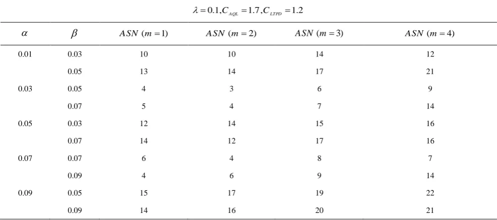
TABLE 1. Optimal values of parameters for different values of  , β and

m

0.1,CAQL 1.7,CLTPD 1.2

  





ASN m( 1) ASN m( 2) ASN m( 3) ASN m( 4)

0.01 0.03 10 10 14 12

0.05 13 14 17 21

0.03 0.05 4 3 6 9

0.07 5 4 7 14

0.05 0.03 12 14 15 16

0.07 14 12 17 16

0.07 0.07 6 4 8 7

0.09 4 6 9 14

0.09 0.05 15 17 19 22

0.09 14 16 20 21

It is seen that the results of proposed MDS sampling plan in the cases of m1 and m2 is near to each other but the results of the cases of m=3 , m=4 are not satisfactory. For instance, assuming 0.05, 0.07, ASN of MDS sampling plan is equal to 14 and 12 in the cases of m1or m2 and ASN is equal to 17 and 18, respectively for the cases of m3and m4.

3. 4. Designing Variable Sampling Plan for Resubmitted Lot The variable sampling plan for resubmitted lots is one of the important sampling plans. Parameters of the proposed sampling plan are as follows:

m= number of resubmissionsn=sample size

a

k =the lower threshold of process capability index for accepting the lot based on the sample

The decision making about received lot based on the process capability index will be as follows:

Step 1: Take a random sample of size

n

and calculated ˆ

pm

C _.

Step 2: If Cˆpmka then accept the lot else, after repeating

the step 2 and resubmitting the lot for

m

times, if the lot was not accepted, then reject the lot.

It is noted that when m =1, then mentioned sampling plan would be similar to a single sampling plan (SSP). So sampling plan for resubmitted lot can be considered as a more general form of SSP.

Sampling plan for resubmitted lots is easy to implement. There are some situations that the producer may discard the results of first sample and take the same number units for inspection and investigation under the

provision of contract. For real example, in many countries such as India, the tax is paid based on the assessment of the first sample and if the producer does not agree with first inspection results then the second result is obtained under the same sample size as in the first inspection.

The OC function of the sampling plan for resubmitted lots is defined as follows (Govindaraju and Ganesalingam [19]):

(16) ( ) 1 (1 )m,

P_A C_pm   P_a

whereCpmis defined as the quality level of submitted lot and Pa is defined as the acceptance probability in a single stage that is obtained as the follows:

(17)

b n

(1+3 ) 2

2 (b n -t)

ˆ _{G - t}

2

0 ₉

[ (t + ξ n ) + (t - ξ n )] dt , k

a

P_a P C_pm k_a

k a

 

 

 

 



 

 _  _  

 

 

 



The ASN of proposed sampling plan for given quality level (Cpm_{) is determined as follows (Govindaraju and}

Ganesalingam [19]):

(18)

(1 (1 ) )

( ) ,

m

n P

a ASN C

pm _P

a

  

Now according to OC function of proposed sampling plan for resubmitted lots and the probability distribution function of Cpm, the required ASN can be minimized by

(19 ( (1 (1 ) )

( )

:

( ) 1

1

( )

2

m

n P_a

Minimize ASN a

P_a

subject to

C_pm C_AQL a a P_A C_AQL

and

C_pm C_LQL a a P_A C_LQL



  



     

    

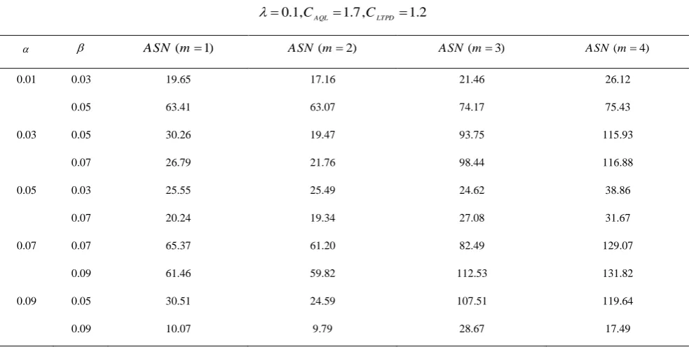
Also a sensitivity analysis is carried out based on different values of

m

to determine which value of

m

has the better performance. The results are presented in Table 2.

It is observed that the ASN of proposed plan in (m2)_{is better than other cases. For instance, for} specified values of 0.05,0.07_{, ASN of MDS} sampling plan is equal to 19.34 in the case of m2 and in other cases of m1,3, 4_{, ASN is equal to 20.24, 27.08} and 31.67, respectively. Thus we have applied the case

(m2)_{for comparison study with other plans.}

Now, we can design variable RGS plan and then compare variable RGS plan with the proposed DSP, MDS sampling plan and variable sampling plan for resubmitted lot.

Now we present methodology to obtain the proposed RGS plan parameters.

In the case of RGS plan with using a grid search, we can determine the minimum ASN plan searching in the multi-dimensional grid formed setting n=3(1)100,

k1=1.0(0.001)1.5, k2=1.5(0.001)2.2.

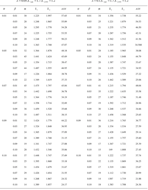
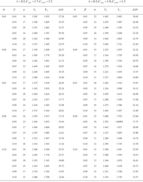
4. SIMULATION STUDIES

Tables 3 and 4 denote the optimal parameters of 1 2

, ,

n k k _{for specified values of} C_{AQL, CLTPD, and}

different values of



and. Since T is the target value

and 2

USL LSL

M  

is the midpoint of the specification

limits, according to the formula





2 2

/

n T

   _{, we}

assumed data comes from standard normal distribution

thus

 

2

n T

 _{and T values can be obtained based on} simulated values of .

For example, if,



0.05,CAQL1.7,CLTPD1.2and

0.05, 0.03

  _{, then the optimal solution is}

1 2

45, 1.441, 1.624

n k  k  _{and the procedure of}

variable RGS plan will be as follows:

Step 1: Collect a sample with n45 observations. Step 2: Accept the lot if Cˆpm1.624 and reject the lot if

ˆ _1.441 pm

C  _{. If} 1.441 ˆ 1.624

pm C

  _{, then repeat steps 1 and 2.}

TABLE 2. Optimal values of parameters for different values of , and m

0.1,C_AQL 1.7,C_LTPD 1.2

  

  ASN m( 1) ASN m( 2) ASN m( 3) ASN m( 4)

0.01 0.03 19.65 17.16 21.46 26.12

0.05 63.41 63.07 74.17 75.43

0.03 0.05 30.26 19.47 93.75 115.93

0.07 26.79 21.76 98.44 116.88

0.05 0.03 25.55 25.49 24.62 38.86

0.07 20.24 19.34 27.08 31.67

0.07 0.07 65.37 61.20 82.49 129.07

0.09 61.46 59.82 112.53 131.82

0.09 0.05 30.51 24.59 107.51 119.64

TABLE 3. Values of optimal parameters for different values ,

0.05,CAQL 1.7,CLTPD 1.2



   0.1,C_AQL1.7,C_LTPD 1.2

 

n

k1 k2 ASN  

n

k1 k2 ASN

0.01 0.01 30 1.225 1.997 57.65 0.01 0.01 34 1.356 1.738 55.22

0.03 28 1.248 1.865 55.89 0.03 25 1.221 1.879 54.53

0.05 26 1.295 1.778 54.28 0.05 21 1.235 1.774 46.50

0.07 24 1.225 1.755 53.55 0.07 20 1.287 1.756 42.31

0.09 20 1.248 1.777 50.23 0.09 36 1.362 1.512 41.56

0.10 24 1.363 1.768 47.07 0.10 34 1.319 1.535 34.588

0.05 0.01 32 1.364 1.878 48.18 0.05 0.01 28 1.185 1.965 38.08

0.03 45 1.441 1.624 45.69 0.03 24 1.155 1.848 44.79

0.05 25 1.354 1.715 38.47 0.05 20 1.387 1.747 33.67

0.07 44 1.487 1.555 46.95 0.07 24 1.135 1.721 34.93

0.09 17 1.226 1.884 38.78 0.09 31 1.436 1.529 27.22

0.10 22 1.349 1.619 37.33 0.10 26 1.462 1.589 25.06

0.07 0.01 45 1.475 1.797 45.84 0.07 0.01 41 1.215 1.794 48.04

0.03 34 1.442 1.698 36.78 0.03 35 1.222 1.635 35.58

0.05 21 1.364 1.776 34.19 0.05 27 1.187 1.746 31.48

0.07 22 1.358 1.716 32.69 0.07 19 1.392 1.712 26.96

0.09 36 1.459 1.520 35.68 0.09 30 1.268 1.537 34.66

0.10 35 1.487 1.511 38.15 0.10 27 1.458 1.568 25.65

0.09 0.01 32 1.424 1.779 44.22 0.09 0.01 36 1.216 1.765 36.77

0.03 27 1.324 1.848 36.95 0.03 20 1.334 1.534 27.59

0.05 24 1.365 1.879 37.09 0.05 27 1.428 1.649 29.14

0.07 20 1.389 1.768 31.15 0.07 21 1.155 1.757 25.60

0.09 19 1.341 1.747 27.08 0.09 17 1.367 1.721 25.39

0.10 28 1.432 1.546 35.06 0.10 15 149 1.808 27.45

0.10 0.01 37 1.448 1.747 37.69 0.10 0.01 33 1.222 1.737 37.74

0.03 25 1.395 1.868 33.18 0.03 22 1.135 1.869 36.25

0.05 31 1.454 1.679 31.67 0.05 17 1.319 1.861 23.67

0.07 29 1.426 1.654 31.55 0.07 19 1.112 1.730 20.99

0.09 16 1.268 1.867 24.32 0.09 14 1387 1.719 21.88

TABLE 4. Optimal values of parameters for different values of ,



0.2,C_AQL 1.7,C_LTPD 1.2

  



0.3,CAQL 1.9,CLTPD 1.3



 n k1

k

2 ASN   n k1 k2 ASN

0.01 0.01 18 1.265 1.935 37.26 0.01 0.01 22 1.462 1.963 29.65

0.03 17 1.248 1.849 32.53 0.03 14 1.435 1.987 26.48

0.05 29 1.357 1.662 31.57 0.05 19 1.448 1.549 24.76

0.07 16 1.269 1.767 29.39 0.07 18 1.359 1.928 23.18

0.09 28 1.362 1.566 24.99 0.09 14 1.564 1.803 22.79

0.10 21 1.337 1.565 22.79 0.10 19 1.465 1.741 21.65

0.05 0.01 17 1.378 1.828 26.27 0.05 0.01 15 1.323 1.875 23.22

0.03 14 1.385 1.779 29.30 0.03 17 1.316 1.795 29.58

0.05 16 1.226 1.991 21.72 0.05 18 1.358 1.765 20.79

0.07 23 1.449 1.565 25.07 0.07 16 1.279 1.924 16.68

0.09 12 1.249 1.845 19.35 0.09 15 1.221 1.835 17.57

0.10 15 1.368 1.616 19.40 0.10 11 1.237 1.804 16.89

0.07 0.01 17 1.375 1.918 26.49 0.07 0.01 28 1.444 1.763 27.07

0.03 19 1.342 1.835 22.24 0.03 15 1.316 1.898 19.13

0.05 28 1.456 1.616 26.19 0.05 22 1.459 1.615 26.98

0.07 16 1.234 1.937 17.77 0.07 17 1.286 1.930 17.68

0.09 24 1.418 1.565 21.88 0.09 25 1.472 1.586 21.24

0.10 17 1.575 1.544 20.81 0.10 14 1.465 1.507 13.89

0.09 0.01 16 1.393 1.913 17.32 0.09 0.01 23 1.488 1.793 23.66

0.03 15 1.365 1.833 19.44 0.03 18 1.355 1.86901 17.75

0.05 17 1.449 1.666 20.83 0.05 19 1.443 1.671 20.98

0.07 19 1.247 1.985 12.61 0.07 15 1.327 1.855 15.88

0.09 9 1.252 1.997 15.54 0.09 11 1.286 1.948 14.74

0.10 18 1.334 1.763 11.24 0.10 12 1.359 1.735 13.78

0.10 0.01 18 1.368 1.928 22.53 0.10 0.01 15 1.348 1.941 22.59

0.03 29 1.449 1.776 23.57 0.03 37 1.588 1.595 34.23

0.05 18 1.355 1.145 18.00 0.05 13 1.346 1.879 16.43

0.07 19 1.419 1.655 19.73 0.07 13 1.468 1.678 19.73

0.09 17 1.376 1.765 15.95 0.09 15 1.341 1.768 13.59

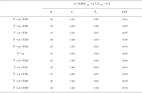
TABLE 5. The optimal parameters for proposed sampling plan (T 



)

0.05,C_AQL 1.7,C_LTPD 1.2

  

n

k1

k

2 ASN

0.5

T    42 1.417 1.587 41.61

0.4

T    44 1.428 1.596 42.85

0.3

T    44 1.431 1.612 44.97

0.2

T  





46 1.428 1.610 43.46

0.1

T  





45 1.437 1.615 45.93

T  45 1.441 1.624 45.69

0.1

T    45 1.445 1.634 46.46

0.2

T    45 1.443 1.631 46.74

0.3

T    47 1.458 1.637 47.46

0.4

T    46 1.461 1.642 48.20

0.5

T  





48 1.463 1.748 49.76

TABLE 6. Results of comparison study under different approaches



 DSP _{MDS sampling plans RGS plan} Sampling plan for resubmitted lots

RGS plan (Wu et al. [11])

0.01 0.025 50.62 19 33.62 38.64 80

0.01 0.075 44.24 17 29.74 32.17 71

0.05 0.01 63.89 16 26.27 28.35 62

0.075 0.025 37.46 10 22.66 23.77 50

0.075 0.10 44.97 14 20.54 34.42 37

0.10 0.05 26.03 13 18.36 21.22 40

0.10 0.075 32.85 9 18.49 19.23 36

0.10 0.10 20.45 8 14.52 23.57 33

Now with regards to the target value (T ) and process mean (



), with assuming T _{, we evaluate}

the process capability index Cˆpm. To analyze the behavior of proposed plan in the case of T 



, we compared the ASN of proposed sampling plan for

different values of T and 0.05,0.03. The results are denoted in Table 5.

5. COMPARISON STUDY AMONG DEVELOPED SAMPLING PLANS

Simulation results under different values of  , and specified value of 0.1,CAQL 1.8,CLTPD 1.1_for probability distribution function are presented in Table 6. It is observed that MDS sampling plan has the least values of ASN and is the best method. RGS plan performs better than sampling plan for resubmitted lots and DSP. DSP has the worst performance in comparison with other sampling plans.

6. CONCLUSION

In this paper, optimization models were developed for designing acceptance sampling plans like RGS, DSP, MDS and sampling plan for resubmitted lots considering consumer risk, producer risk as the constraints and process capability index as the performance measure. The proposed plan was based on exact probability distribution of process capability index. In addition, we presented a procedure to obtain the required sample size, and the thresholds of process capability index to make decision about the lot.

It is observed that MDS sampling plan has the least values of ASN and is the best method. RGS plan performs better than sampling plan for resubmitted lots and DSP. DSP has the worst performance in comparison with other sampling plans.

7. REFERENCES

1. Jennett, W. and Welch, B., "The control of proportion defective as judged by a single quality characteristic varying on a continuous scale", Supplement to the Journal of the Royal Statistical Society, Vol. 6, No. 1, (1939), 80-88.

2. Moskowitz, H. and Tang, K., "Bayesian variables acceptance-sampling plans: Quadratic loss function and step-loss function",

Technometrics, Vol. 34, No. 3, (1992), 340-347.

3. Pearn, W. and Wu, C.-W., "Critical acceptance values and sample sizes of a variables sampling plan for very low fraction of defectives", Omega, Vol. 34, No. 1, (2006), 90-101. 4. Wu, C.-W., "Assessing process capability based on bayesian

approach with subsamples", European Journal of Operational

Research, Vol. 184, No. 1, (2008), 207-228.

5. Balamurali, S., Aslam, M. and Jun, C.-H., "A new system of skip-lot sampling plans including resampling", The Scientific

World Journal, Vol. 2014, (2014).

6. Wu, C.-W., Aslam, M. and Jun, C.-H., "Variables sampling inspection scheme for resubmitted lots based on the process capability index Cpk", European Journal of Operational

Research, Vol. 217, No. 3, (2012), 560-566.

7. Suresh, K. and Sangeetha, V., "Construction and selection of bayesian chain sampling plan (BChSP-1) using quality regions",

Modern Applied Science, Vol. 5, No. 2, (2011).

8. Aslam, M., "Double acceptance sampling based on truncated life tests in rayleigh distribution", Editorial Advisory Board e, Vol.

17, No. 4, (2005), 605-610.

9. Sherman, R. E., "Design and evaluation of a repetitive group sampling plan", Technometrics, Vol. 7, No. 1, (1965), 11-21. 10. Aslam, M., Azam, M. and Jun, C.-H., "A mixed repetitive

sampling plan based on process capability index", Applied

Mathematical Modelling, Vol. 37, No. 24, (2013),

10027-10035.

11. Wu, C.-W., Aslam, M., Chen, J. C. and Jun, C.-H., "A repetitive group sampling plan by variables inspection for product acceptance determination", European Journal of Industrial

Engineering, Vol. 9, No. 3, (2015), 308-326.

12. Aslam, M., Azam, M. and Jun, C. H., "Various repetitive sampling plans using process capability index of multiple quality characteristics", Applied Stochastic Models in Business

and Industry, Vol. 31, No. 6, (2015), 823-835.

13. Aslam, M., Yen, C.-H. and Jun, C.-H., "Variable repetitive group sampling plans with process loss consideration", Journal of Statistical Computation and Simulation, Vol. 81, No. 11, (2011), 1417-1432.

14. Suresh, K., Umamaheswari, S. and Veerakumari, K. P., "Bayesian repetitive deferred sampling plan indexed through relative slopes", (2014).

15. Wortham, A. and Baker, R., "Multiple deferred state sampling inspection", The International Journal of Production

Research, Vol. 14, No. 6, (1976), 719-731.

16. Soundararajan, V. and Vijayaraghavan, R., "Construction and selection of multiple dependent (deferred) state sampling plan",

Journal of Applied Statistics, Vol. 17, No. 3, (1990), 397-409.

17. Vaerst, R., "A procedure to construct multiple deferred state sampling plan", Methods of Operations Research, Vol. 37, (1982), 477-485.

18. Aslam, M., Azam, M. and Jun, C.-H., "Multiple dependent state sampling plan based on process capability index", Journal of

Testing and Evaluation, Vol. 41, No. 2, (2013), 1-7.

19. Govindaraju, K. and Ganesalingam, S., "Sampling inspection for resubmitted lots", Communications in Statistics-Simulation

and Computation, Vol. 26, No. 3, (1997), 1163-1176.

20. Aslam, M., Wu, C.-W., Azam, M. and Jun, C.-H., "Variable sampling inspection for resubmitted lots based on process capability index cpk for normally distributed items", Applied

Mathematical Modelling, Vol. 37, No. 3, (2013), 667-675.

21. Balamurali, S., Park, H., Jun, C.-H., Kim, K.-J. and Lee, J., "Designing of variables repetitive group sampling plan involving minimum average sample number", Communications in Statistics—Simulation and Computation®, Vol. 34, No. 3, (2005), 799-809.

22. Balamurali, S. and Jun, C.-h., "Repetitive group sampling procedure for variables inspection", Journal of Applied Statistics, Vol. 33, No. 3, (2006), 327-338.

23. Nezhad, M. S. F. and Seifi, S., "Designing optimal double-sampling plan based on process capability index",

Communications in Statistics-Theory and Methods,

just-accepted, (2016), 00-00.

24. Balamurali, S. and Subramani, J., "Designing of variables repetitive group sampling plan indexed by point of control",

Journal of Manufacturing Engineering, Vol. 5, (2010), 166-169.

25. Chan, L. K., Cheng, S. W. and Spiring, F. A., "A new measure of process capability: Cpm", Journal of Quality Technology, Vol. 20, No. 3, (1988), 162-175.

26. Balamurali, S. and Jun, C.-H., "Multiple dependent state sampling plans for lot acceptance based on measurement data",

European Journal of Operational Research, Vol. 180, No. 3,

Designing Different Sampling Plans Based on Process Capability Index

M. S. Fallah Nezhad, S. Seifi

Faculty of Industrial Engineering, Yazd University, Yazd, Iran

P A P E R I N F O

Paper history: Received 31 October 2015

Received in revised form 08 June 2016 Accepted 14 July 2016

Keywords:

Process Capability Index

Repetitive Group Sampling Plan (RGS) Acceptance Sampling Plan

Average Sample Number (ASN)

A Multiple Dependent State (MDS) Sampling Plan

Double Sampling Plan

هديكچ

لذم یاَ رادزب ٍوًمو ی شزیذپ تُج ٌدزتسگ رًط ٍب

ا ی تکزض رد اَ ازب ی سرا یبای ىچمَ ي ماخ داًم هی

اُو تلاًصحم یی

مَ رد .تسا ٌذض ٌدافتسا هی

لباق صخاض ،لاح تی

آزف ذىی (

PCIS

حم رد ) طی اَ ی تعىص ی ناًىع ٍب فلتخم رایعم

اواًت یی

ب ٍک تسا ٌذض ٌدافتسا یاىبم ز

ازف جيزخ ذىی سا کی ،فذَ ٌدساب آزف ذىی تابث ، ذىیازف ي فلاتا آزف ذىی یم تسد ٍب ذیآ رد .

ا هی رازکت ٌيزگ ٍوًمو حزط اذتبا ،صَيژپ ی

(

RGS

لباق صخاض ساسا زب ) تی

آزف ذىی ازب ی غتم یاَزی سرساب ی ٍعسًت ٍتفای

اپ سپس .تسا اَزتمار

ی ُب ٍىی ی حزط

RGS

پ یداُىطی عت هیی ٌذض ىچمَ ي هی رادزب ٍوًمو حزط تلاح ی

یاَ ٍتسباي

ذج ٍواگذىچ ذی

(

MDS

) ، کی ٍوًمو حزط یرادزب يد ٍواگ (

DSP

ي ) کی ٍوًمو حزط یرادزب ازب ی ٌيزگ یرازکت یاَ ٍعسًت

ٍتفای اُو رد ي ،تی کی ٍعلاطم ی اقم ٍسی یا ب هی حزط ٍوًمو اَ ی پ یداُىطی یم ماجوا دًض اتو ي یم ٌداد حیضًت جی ذوًض

.