OPTIMAL SOLUTION IN A CONSTRAINED DISTRIBUTION SYSTEM
M. Modarres
Department of Industrial Engineering, Sharif University of Technology Tehran, Iran, [email protected]
E. Taimury
Department of Industrial Engineering, Iran University Science and Technology Tehran, Iran, [email protected]
(Received: April 7, 2001 – Accepted in Revised Form: December 31, 2001)
Abstract We develop a method to obtain an optimal solution for a constrained distribution system with several items and multi-retailers. The objective is to determine the procurement frequency as well as the joint shipment interval for each retailer in order to minimize the total costs. The proposed method is applicable to both nested and non-nested policies and ends up with an optimal solution. To solve this large nonlinear and integer problem, a two-level algorithm is proposed. In the first level, the functional constraints are relaxed and a solution is obtained by taking advantage of its special structure. Then, we apply separable programming technique for finding the optimal solution of the original problem. To decrease the size of the problem, some appropriate bounds on variables are introduced. We will show that under some conditions, the optimal solution of the original problem is proportional with the solution of its unconstrained problem.
Key Words Production/Inventory, Constrained Problems, Separable Programming, Supply Chain, Nested
ﻩﺪﻴﻜﭼ
ﻲﻣﻪﻌﺳﻮﺗﻊﻳﺯﻮﺗﻪﻜﺒﺷ ﻚﻳﻪﻨﻴﻬﺑ ﺏﺍﻮﺟﻥﺩﺭﻭﺁﺖﺳﺪﺑﻱﺍﺮﺑﻲﺷﻭﺭ،ﻪﻟﺎﻘﻣﻦﻳﺍﺭﺩ
ﺪﺑﺎﻳ
. ﻪﻜﺒﺷﻦﻳﺍﺭﺩ
ﺭﺎﺒﻧﺍﻖﻳﺮﻃﺯﺍﺲﭙﺳﻭﻱﺭﺍﺪﻳﺮﺧﻱﺰﻛﺮﻣﺭﺎﺒﻧﺍﻚﻳﻂﺳﻮﺗﻱﺩﺪﻌﺘﻣﻡﻼﻗﺍﻪﻛ
ﻲﻋﺮﻓﻱﺎﻫ
)
ﻲﺷﻭﺮﻓﻩﺩﺮﺧ
(
ﻊﻳﺯﻮﺗ
ﻲﻣ
ﺩﻮﺷ
ﺖﺳﺍﻱﺩﺪﻌﺘﻣﻱﺩﺮﻛﺭﺎﻛﻱﺎﻬﺘﻳﺩﻭﺪﺤﻣﻱﺍﺭﺍﺩ
.
ﺭﺎﭘ،ﺎﻬﻨﻳﺍ ﺮﺑﻩﻭﻼﻋ ﺮﺘﻣﺍ
ﻲﻣﺰﻴﻧﻝﺪﻣﻱﺎﻫ
ﻲﻌﻄﻗﺮﻴﻏﺪﻨﻧﺍﻮﺗ
)
ﻲﻟﺎﻤﺘﺣﺍ
(
ﺪﻨﺷﺎﺑ
. ﺯﺍﻲﻟﺍﻮﺘﻣﻞﻤﺣﻭﺩﻦﻴﺑﻲﻧﺎﻣﺯﻪﻠﺻﺎﻓﻦﻴﻨﭽﻤﻫﻭﻱﺰﻛﺮﻣﺭﺎﺒﻧﺍﺭﺩﻡﻼﻗﺍﺪﻳﺮﺧﺮﺗﺍﻮﺗﻦﻴﻴﻌﺗ،ﻑﺪﻫ
ﻪﻨﻳﺰﻫﻉﻮﻤﺠﻣ ﻪﻛ ﻱﺭﻮﻄﺑ،ﺖﺳﺍ ﻲﻋﺮﻓ ﻱﺎﻫﺭﺎﺒﻧﺍ ﺯﺍ ﻡﺍﺪﻛ ﺮﻫ ﻪﺑ ﻱﺰﻛﺮﻣ ﺭﺎﺒﻧﺍ
ﺩﺩﺮﮔﻞﻗﺍﺪﺣ ﺎﻫ
. ﻙﺮﺘﺸﻣﻪﻟﻮﻤﺤﻣ
ﻪﺑﻱﺰﻛﺮﻣﺭﺎﺒﻧﺍﺯﺍﺎﻫﻻﺎﻛ
ﻲﻣﻒﻠﺘﺨﻣﻱﻻﺎﻛﺪﻨﭼﻞﻣﺎﺷﻲﻋﺮﻓﻱﺎﻫﺭﺎﺒﻧﺍ ﺩﻮﺷ
. ﻱﺎﻬﺘﺳﺎﻴﺳﻱﺍﺮﺑﻢﻫﻱﺩﺎﻬﻨﺸﻴﭘﺵﻭﺭ
Nested
ﺩﺭﺍﺩﺩﺮﺑﺭﺎﻛﻥﺁﺮﻴﻏﻱﺍﺮﺑﻢﻫﻭ
. ﺢﻴﺤﺻﺩﺪﻋ،ﻲﻄﺧﺮﻴﻏﻱﺰﻳﺭﻪﻣﺎﻧﺮﺑﻚﻳﻪﺑﻪﻛﻞﺻﺎﺣﻲﺿﺎﻳﺭﻝﺪﻣﻱﺍﺮﺑ
ﻩﺯﺍﺪﻧﺍﺎﺑ
ﻲﻣﻲﻬﺘﻨﻣﮒﺭﺰﺑﻱﺎﻫ
ﻩﮋﻳﻭﻢﺘﻳﺭﻮﮕﻟﺍ،ﺩﻮﺷ
ﻲﻣﻲﺣﺍﺮﻃﻱﺍ
ﺖﺳﺍﻪﻠﺣﺮﻣﻭﺩﻱﺍﺭﺍﺩﻪﻛﺩﻮﺷ
.
ﺩ
،ﻝﻭﺍﻪﻠﺣﺮﻣﺭ
ﻩﺮﻬﺑﺎﺑﻭﻱﺩﺮﻛﺭﺎﻛﻱﺎﻬﺘﻳﺩﻭﺪﺤﻣﻱﺯﺎﺳﺩﺍﺯﺁﺎﺑ ﻲﻣﺖﺳﺪﺑﻪﻴﻟﻭﺍﺏﺍﻮﺟﻚﻳﻥﺁﻩﮋﻳﻭﺭﺎﺘﺧﺎﺳﺯﺍﻱﺮﻴﮔ
ﺪﻳﺁ
.
ﺭﺩ،ﻩﺎﮕﻧﺁ
ﻪﻣﺎﻧﺮﺑﺯﺍﻩﺩﺎﻔﺘﺳﺍﺎﺑﻡﻭﺩﻪﻠﺣﺮﻣ
ﻲﻣﻪﺒﺳﺎﺤﻣﻲﻠﺻﺍﻪﻟﺎﺴﻣﻪﻨﻴﻬﺑﺏﺍﻮﺟ،ﺮﻳﺬﭘﻚﻴﻜﻔﺗﻱﺰﻳﺭ ﺩﻮﺷ
.
ﻥﺩﺮﻛﺩﻭﺪﺤﻣﻱﺍﺮﺑ
ﻠﺣﺮﻣﺭﺩ،ﻥﺁﻥﺩﻮﻤﻧﻞﺣﻞﺑﺎﻗﻭﻪﻟﺎﺴﻣﻩﺯﺍﺪﻧﺍ
ﻡﺍﺪﻛﺮﻫﻱﺍﺮﺑﺐﺳﺎﻨﻣﻦﻴﻳﺎﭘﺪﺣﻚﻳﻭﻻﺎﺑﺪﺣﻚﻳﻢﺘﻳﺭﻮﮕﻟﺍﻡﻭﺩﻪ
ﺮﻴﻐﺘﻣﺯﺍ
ﻲﻣﻦﻴﻴﻌﺗﺎﻫ ﺩﺩﺮﮔ
.
ﻲﻣﻩﺩﺍﺩﻥﺎﺸﻧﺎﻨﻤﺿ
ﺎﺑﺐﺳﺎﻨﺘﻣﻲﻠﺻﺍﻪﻟﺎﺴﻣﻪﻨﻴﻬﺑﺏﺍﻮﺟﺹﺎﺧﻂﻳﺍﺮﺷﺖﺤﺗﻪﻛﺩﻮﺷ
ﺖﺳﺍﺖﻳﺩﻭﺪﺤﻣﻥﻭﺪﺑﻪﻟﺎﺴﻣﻪﻨﻴﻬﺑﺏﺍﻮﺟ
.
1. INTRODUCTION
In supply chain or logistics approach, a major goal of all world-class companies is to reduce the total cost of the system altogether rather than to minimize inventory or transportation cost, separately. In this paper, we study a distribution system with a central as well as various local (or departmental) warehouses, in which different items are flowing from outside
into the central warehouse and then shipped to the departmental warehouses for the final distribution. There are many constraints resulting from limited resources. The objective is to reduce the integrated cost of inventory and transportation altogether by determining the optimal shipment planning, i.e. the interval time between two successive shipments for each item.
be applied to represent a company that produces several products and distributes them through many retailers.
Maxwell and Muckstadt [3] formulated a model for multi-echelon problems and developed a method on the basis of graphical structure of the model. Later, Muckstadt and Roundy [5] simplified the method for the case of multi-item, multi-retailer production-distribution system. However, they assumed nested policies hold, only. Modarres and Taimury[4] developed another method when this assumption is relaxed, although it may hold for some nodes. Jackson et al. [2] proposed a method for a constrained distribution system on the basis of Lagrangian relaxation. However, this method works only if the coefficients of constraints are proportional to the corresponding holding or setup costs. Furthermore, if there is more than one constraint, then the number of iterations will tend to infinity. Although they claim the method is convergent, it cannot be proved mathematically. Bertrand and Bookbinder [1] considered a two-echelon periodic review inventory system consisting of a warehouse W and non-identical retailers R1, …, Rn. In their model, it is possible
to redistribute among retailers, between replenishment of the overall system. Heijeden [6] developed an inventory control rule for a multi-echelon system with a stock central depot. The control rule determines a set of rationing fractions at the central depot as well as a set of order-up-to levels for retailers.
In this paper, we propose a method for a constrained distribution system, similar to the model of Jackson et al.[2], but with no restriction on the coefficients of the constraints. The resulting solution obtained from our method is optimal within any desired measure of accuracy.
The remainder of this paper is organized in the following way. In the next section, we present the definition of the problem along with the assumptions, as well as the graphical structure of the model according to our notation. In section 3, the framework of the method as well as its structure of the model, which consists of two levels, is presented. In sections 4, we illustrate how to obtain the optimal solution of the unconstrained problem in the first level, as well as mathematical developments regarding the properties of this optimal solution. In
sections 5, we present the second level of the method and how to apply separable programming with less effort. The summary of the proposed algorithm is developed in section 6.
2. THE PROBLEM
Consider a multi-echelon inventory system carrying I type of items. This system consists of one central warehouse and M retailers (departmental warehouses). The purchased items are stocked in the (central) warehouse first and then shipped to the retailers. Shipments to each retailer may include different items. In other words, joint replenishment to retailers is assumed. In this system, one may consider various functional constraints, such as the amount of inventory (total or average) or the maximum number of orders from outside.
The objective is to determine the procurement frequency as well as the joint shipment interval for each retailer in order to minimize the total inventory costs, including setup and holding costs while different constraints are satisfied.
We do not restrict the policy to be nested only. However, it is assumed to be stationary. By stationary, we mean the reorder points for each warehouse is invariant with respect to time. We also assume the interval time between two successive orders for each item and in all warehouses is a power-of-two multiple of a base planning period. By our experience, the most practical base planning period is one week.
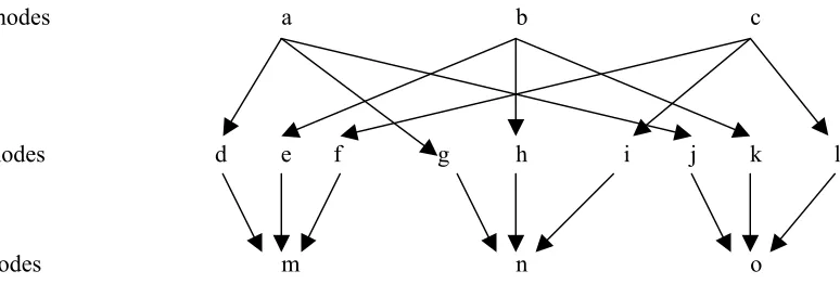
The system illustrated in figure 1 has three items. Nodes a, b and c represent the storage of these items in the central warehouse. There are also three retailers. In this figure, nodes d, e and f represent the receipt of items a, b and c, respectively, at retailer 1. Similarly, nodes g, h, i as well as nodes j, k, l represent the receipt of the same items at retailers 2 and 3, respectively. On the other hand, nodes m, n and o indicate joint shipment of items to retailers 1,2 and 3, respectively.
Assumptions and Notation
We use the following notation for node n, for n = 1, ...., N.dn : demand rate at node n;
Sn : set up (or ordering) cost of node n. This cost is
applicable for all nodes;
hn : holding cost of an item at node n. This cost is
proportional to the level of inventory, not applicable to J nodes;
T(n) : the inter-shipment time (between two successive shipments) at node n;
T*(n) : the optimal inter-shipment time at node n; τ (n) : the optimal inter-shipment time at node n, when functional constraints are relaxed.
We assume H represents the set of functional constraints. Then, associated for constraint h
∈
H, the following notation is also introduced.bh : maximum amount of hth resource;
N(h): the set of nodes in constraint h;
Aih: the consumption coefficient of node i in
constraint h.
Clearly, a node may be in more than one constraint. In other words, for h1, h2
∈
H, theintersection of N(h1) and N(h2) is not necessarily
empty.
Note
We assume demand rate at each node is constant. Although this assumption is justified for retailers, it may seem to be unrealistic especially for W type of nodes. However, we assume the demand at each retailer shifts to the central warehouse, immediately. Therefore, the demand for each node of W type is also assumed to be constant. On the other hand, since the number of retailers is usually very large, the inventory cost can be approximated with the cost function of a system with continuous demand, see Muckstadt and Roundy [5].Nested and Non-Nested Policies
A policy is called nested if T(i)≥
T(j), where i precedes j in the graph. By our notation, with the existence of nested relation between two successive nodes, they are connected by a directed arc. In other words, if no arc connects nodes, then nested relation does not hold at all and each node is independent of the rest of the system and can be optimized independently. However, since we assume replenishment to retailers includes several items jointly and power-of-two policy also holds, then at least nested property holds between R and J nodes. Some nested relations may also exist, due to technological or other restrictions.Considering this concept and notation, the set of arcs, A(G) , represents the nested relations in the problem. Therefore, for any arc of the graph, the following relation holds.
Wnodes a b c
R nodes d e f g h i j k l
Jnodes m n o
Typical Constrained Models
Depending on the type of constraints, we define two constrained models.Model I
H h b ) i ( T a .t . s ) n ( T g ) n ( T S Minimize h ) h ( N i ih ) G ( N n n n ∈ ≤ +∑
∑
∈ ∈ (1) ) G ( A ) j ,i ( ), j ( T ) i (T ≥ ∈ (2)
). G ( N j , o ) j ( T ) G ( A i ,..., 2 , 1 , 0 l , B 2 ) i ( T l ∈ ≥ ∈ =
= (3)
where, gn = (hn.dn)/2. In fact, gn represents the holding
cost of one unit of item per period in node n. B denotes the base planning period.
It is obvious from the model that all functional constraints of (1) are linear and the objective function is convex as well as separable.
Model II
In this model, Constraints 1 are replaced by the following constraints.H h b ) i ( T a h ) h ( N i
ih ≤ ∈
∑
∈
(4)
Constraints
Inequalities 1 or 4 represent functional constraints, (2) indicates nestedness relation while power-of-two constraints are represented by (3). In the remaining part of this paper by constraints, we mean functional constraints of (1) or (4) only and not nested of (2) or power-of-two of (3) constraints.Many real-world restriction can be expressed by either constraints (1) or (4) of models I or II, such as the maximum allowable amount of inventory (capital tied up with stocks) or the maximum number of orders from outside are of special importance. The restriction for capital tied up with stocks can be applied either for the total system or for each retailer. The former case occurs when the inventory system is an integrated one and operated by a single organization. In the
latter case, retailers are independent, such as in a supply chain system, in which retailers are restricted by a maximum amount they can invest for their stocks. The following examples fit in either model I, or model II.
Example 1. Restriction on the Average
Investment in Inventory
Suppose the policy is to keep the average amount of total inventory under a certain amount of B. This means the following constraint has to be satisfied. B 2 Q C ) G ( N j j j ≤∑
∈where, Cj is the unit price and Qj is the ordering
size of node j. Since Qj = dj T(j) and gj = (hjdj) /2
and also by considering the fact that Cj/hj is the
same for every j, then the above constraint changes to: b ) j ( T g ) G ( N j j ≤
∑
∈ (5)where, b=B(hj/Cj).
In this example, H= {1} and ajh=gj for j=1,.N.
If Cj/hj is not the same for every j, then
a
jh≠
g
j, and the method by Jackson et.al.[1] is not applicable, any more.Example 2. Distribution System With Restricted
Average Inventory for Retailers
Suppose the average amount of inventory for each retailer is restricted. Then, similar to example 1, for each retailer, a constraint such as (5) holds. In other words, we have,H h , b ) j ( T a h ) h ( N
j∈
∑
jh ≤ ∈n ) j ( T
1 W j
≤
∑
∈
where, W is the set of nodes in central warehouse and n is the maximum number of allowable orders. This is a model of type II. To solve this model, we substitute 1/T(j) with T'(j) as mentioned before, and apply the proposed algorithm.
3. FRAMEWORK OF THE METHOD
In this section, we first present the main steps of the proposed method for Model I. To solve this problem, power-of-two constraints of (3) are relaxed and then a two-levels algorithm is applied, as follows:
Level 1.
The functional constraints of (1) are relaxed and then the optimal solution is obtained, by using the method developed by Modarres and Taimury [4].Level 2.
The optimal solution of Model I is obtained by applying separable programming. In this level, upper and lower bounds of variables are determined by using the solution obtained in the first level.It is necessary to explain why we do not apply separable programming directly to obtain the solution and go through a two levels algorithm. In separable programming, each variable is substituted with some bounded variables in order to linearize the functions. The number of substituted variables depends on the domain of the original variable. Thus, it is vital to shorten that domain. On the other hand, determining a reasonable upper and lower bound for variables is not an easy task. In other words, if the variation range of a variable is not known, then the number of substituted new variables increases indefinitely, or at least it will be so large that makes it out of control.
In our proposed method, the results of level 1 of the algorithm as well as some other technical properties are used to shorten the variation range and to decrease the number of new variables, and consequently the size of the linear problem.
After the optimal reorder intervals, T*(n),
n∈N(G), corresponding to the problem with relaxed
constraints of power-of-two is determined, then each reorder interval is changed into 2l B, where, l
is the smallest integer such that the following relation for each n∈N(G), holds.
1 l 1
l l
l 2 g(n)2
) n ( K 2 ) n ( g 2
) n (
K +
+ +
≤
+ (6)
One should note that any model that includes power-of-two constraints is quite complicated to be solved by standard integer programming techniques. For more detail, the reader is referred to Maxwell and Muckstadt [3].
Transforming Model II into Model I
To solve model II, in the first level and after relaxing constraints (4), T(n) is substituted with 1/T’(n).Thistransforms it into Model I, which enables us to use the same procedure as that model. In the second level, the optimal solution is used in model II directly, since constraint (4) is appropriate for applying separable programming. Therefore, in the remaining part of this paper we concentrate on how to solve Model I.
4. LEVEL 1 - SOLUTION PROCEDURE
According to the method developed by Muckstadt and Roundy [5] and also by Modarres and Taimury [4], in any solution (including optimal) nodes are divided into some sets called "clusters".
Definition 1
a) A cluster is a set of nodes with equal inter-arrival or inter-shipment time. If s is a cluster, then inter-shipment of all nodes of this cluster is T(s).
b) In any solution, the clusters of a constraint are defined as the set of clusters containing at least one node of that constraint.
On the basis of definition 1, for any particular solution, the following notation is introduced. C: set of clusters;
Ch : set of clusters of constraint h ∈ H;
H(s): set of constraint containing at least one node of s ∈ C;
; h a ) h , s ( A )} s ( H ) h ( N { i i
∑
∩ ∈ =G(X): sum of gi associated with set X ;
S(X) : sum of ki associated with set X, i.e.
∑
∑
∈ ∈ = = X i i X ii; and S(X) S g
) X ( G
Lemma 1
. Suppose s and s' are two clusters in the optimal solution and T(s') < T(s). Then, the direction of any arc connecting a node of s to a node of s' is always from s to s'.Proof:
If not, then it contradicts the definition of arcs in our system.Marginal Costs
Definition 2.
Let T be the inter-shipment of all nodes of cluster s. Then, the marginal cost of this cluster called MT(s), is defined to be the derivativeof its cost with respect to T(s). Therefore,
) s ( T ) s ( S ) s ( G ) s (
MT = − 2 (7)
Marginal cost represents the incremental rate of cost with respect to increasing inter-shipment of that cluster.
Optimal Inter-Shipment of Unconstrained
Problems
If no node of cluster s belongs to any constraint, then, the minimum value of this convex function occurs at MT (s) = 0. In other words, theoptimal inter-shipment for this cluster is as follows:
) s ( G ) s ( S ) s ( =
τ (8)
Definition 3.
We define relative marginal cost of cluster s with respect to a constraint h, denoted by mT(s, h) as follows.) h , s ( A ) s ( M ) h , s (
mT = T
where, T is the inter shipment of this cluster.
Theorem 1.
If no cluster of h∈
H has any node in other constraints, then the optimal relative marginal cost of every cluster of this constraint is the same.Proof:
For clusters s∈
C_h and s'∈
Ch, let mT(s,h) < mT (s',h ). Then, increase T(s) by ∆T and
decrease T(s') by
) h , s ( A ) h , s ( A T ′
∆ . Clearly, constraint h is still satisfied but the total cost decreases. Thus, s and s' are not part of an optimal solution.
Definition 4.
Relative Importance of cluster s in relation with constraint h is defined as follows:) h , s ( A ) s ( G sh = τ
Definition 5.
For each constraint say h∈
H,we define overcapacity coefficient denoted by αh as
follows:
∑
∑
∈ ∈ τ = α h h C t C th A(,lh) (l) ) l ( T ) h ,l ( A (9)
By this definition, the constraint is satisfied if the available resource is increased from bh to αh bh.
Clearly, for any active constraint, αh > 1.
Theorem 2.
If no cluster of h∈
H has any node in other constraints and for every node in N(h) the objective function has the form of Si /T(i) + gi T(i),then the value of the following term is constant for every cluster of this constraint.
τ −
τ ) 1
) s ( * T ) s ( ( 2
sh (10)
Proof:
From theorem 1 and also by replacing MT(s) from (7) and also considering (8), the result is obtained.
importance of all clusters of constraint h is the same, then the optimal solution is proportional with the optimal solution obtained from the first level. In other words,
h ) s ( ) s ( * T
α τ
= (11)
Proof:
From (10).Note:
The result of Corollary 1 is a generalization of the main result of Maxwell and Muckstadt [3] for single constraint. They reached the same result by applying Lagrangian relaxation technique.Example 4.
Consider the example presented in Jackson et al. [2], illustrated by figure 1. Holding and set up costs associated with nodes are shown in the Table 1. We assume nested policies holdin this example, for every successive pair of nodes. However, the following constraint also has to be considered.
8T(a) + T(b) + T (c) + T (d) + 3 T (e) + 5T(f) + T(g) + T(h) + T(i) +2T (j) +6 T (k) + T (l)
≤
25.Solution:
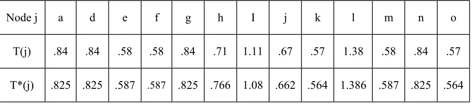
The optimal solution for this problem, τ(s), after relaxing its single constraint, is obtained by applying the method proposed by Modarres and Taimury[4] and is shown in the following table. On the other hand, since the consumption coefficient for each variable is equal to the corresponding gn,then, the relative importance of all clusters is the same. Therefore, the result of corollary 1 can be applied. By our definition, α1 = (27.9)/(25). The
optimal inter-shipment for each cluster, T*(s), is
also shown in the Table 2.
Example 5
. Consider example 4, again. However, this time consider the following constraints. T(d) + 3T(e) + 5T(f)≤
3,T(g) + T(h) + T(i)
≤
4, 2T(j) + 6T(k) + T(l)≤
4.As can be seen from Table 1, the clusters of the 3rd constraint, or nodes (j, k, l, o) are not in any other constraints. Furthermore, rs3 =1 for all clusters of this
constraint. Therefore, in this case, T*(j) = τ (j)/ α 1,
where α3 = 1.65. Thus, T*(j) = 0.4 , T*(k) = 0.35, T*(l)
= 1.05, T*(o) = 0.35.
5. LEVEL II - FOUNDATION AND PROCEDURE
In this level, the optimal solution is determined by separable programming, starting with the solution obtained from level I. To do that, we linearize the objective function, which is a separable function. TABLE 1. Set Up and Holding Cost of the Nodes of Example 1.
Nodes a b c d e f g h i j k l m n o
Sn 1 4 3 2 1 1 1 1 2 1 1 3 2 5 1
gn 8 1 1 1 3 5 1 1 1 2 6 1 - - -
TABLE 2. Optimal Inter-Shipment of Clusters.
Cluster Nodes τ(s) T*(s)
1 (k), (o)
3
3 0.517
2 (e), (f),
(m), (j)
2
2 0.634
3 (a), (d),
(g), (n)
0
.
9
0.85
4 (h) 1 0.896
5 (i)
2
1.2676 (c), (l)
3
1.552On the other hand, since the constraints are also linear functions, then the resulting model is a linear programming problem and can be solved by simplex method with bounded variables. In fact, each variable is replaced with some new variables within an upper and a lower bound. The number of substituted variables for each original variable depends on the variation range of that variable and also on the desired accuracy of the solution. Naturally, this number can be increased tremendously. To avoid facing with a huge problem, two points should be considered.
a. To have fewer variables, it is necessary to shorten the variation range of variables as much as possible. We recall that in a convex separable programming, when the optimal solution does not lie on the border of a specified variation range, then that solution is still optimal even if the range is enlarged. However, if the solution lies on the border, then enlarging the range may lead to a better solution. Therefore, finding an appropriate initial range for each variable is an important task in this method.
b. Since the accuracy of the solution depends on the number of substituted variables, first we obtain an optimal solution with less accuracy and then increase the number of these variables in the neighborhood of the optimal solution for fine-tuning.
As mentioned before, to determine a reasonable variation range for each variable, we obtain the optimal solution and identify the clusters, after relaxing the functional constraints.
Notation:
Let T(s,h) and T(s,h) be the lower and upper bound of T*(s), respectively, if there is
only one constraint, h
∈
H(s).The following theorem is a guideline for selecting reasonable upper and lower bounds for variables.
Theorem 3.
Consider a constraint h∈
H, such that none of its clusters belongs to any other constraints, then the variation range of inter-shipment of clusters of this constraint is obtained as follows.1 ) 1 ( r ) h ( R ) s ( ) h , s (
T 2h
sh α − +
τ
= (12)
and, 1 ) 1 ( r r ) s ( ) h , s (
T 2h
sh
h α − +
τ
= (13)
where, }, C u , r max{ ) h (
R = uh ∈ h
and, }. C u , r min{ ) h (
r = uh ∈ h
Proof:
Let. C s , ) s ( * T ) s ( ) v ( * T ) v ( h ∈ τ ≥ τ
Then, from (9) it is implied that
) v ( * T ) v ( h ≤ τ
α .
Similarly, r(h) = rvh results from (10) and also from
the definition of cluster v. On the other hand, from (10), 1 } 1 ] ) v ( T ) v ( {[ r r ) s ( * T ) s ( 2 uh uh 2 + − τ =
τ (14)
Now, by substituting rvh with r(h) and considering
) v ( * T ) v ( h ≤ τ
α in (14) the proof for (13) is complete. The proof for (12) is similar.
Variation Range of a Cluster Inter-Shipment
Let, Tu(s) and Tl(s) denote the upper and lower bound of T*(s), respectively, when all constraintscontaining at least one node of s are considered. Then, )} s ( H h ), h , s ( T min{ ) s (
Tl = ∈
and, )}} s ( H h ), h , s ( T max{ ), s ( min{ ) s (
Tu = τ ∈
τ(s), (the unconstrained optimal solution), therefore, τ(s) is considered as the ceiling for the upper bound of this variable, in (16).
Enlarging Variation Range of Variables For a cluster of s
∈
C, we assign a lower bound from (15) and an upper bound from (16). However, enlarging this range may results in a better solution if the optimal solution lies outside of this range. To make sure the variation range is large enough, we change the upper or lower bound of a variable if its value is exactly equal to either limits of the range. If the value of a variable is equal to the upper (or lower) limit of the border, then we set τ(.) (or 0) as the new upper (or lower) bound for this variable.It is necessary to mention that only in very few cases out of many we examined, enlarging the variation range was required.
6. THE ALGORITHM
In this section, we summarize the results of the preceding section into an algorithm. Set δ as the measure of accuracy of each variable of the optimal solution.
Step 1.
Relax functional as well as power-of-two constraints and apply the method proposed by Modarres and Taimary[4] to solve the problem. However, do not merge the clusters that have equal inter-shipments. Identify all clusters s∈
C as well as H(s). (For model II, in this step the original problem is solved and then T(n) is substituted by 1/T'(n) from Step 2 on.)Step 2.
For each constraint h∈
H, determine αh,R(h) and r(h) independently. If αh
≤
1 for every h∈
H, then the constraints are satisfied and the solution is optimal. Go to Step 9.Step 3.
If there exits only one constraint, H= {h}, and all C is the same for every j∈
N, then we have,h ) j ( ) j ( * T
α τ =
Go to Step 9.
Step 4.
If no cluster of a constraint h∈
H, belongs to any other constraint and also αh is thesame for every cluster of this constraint, then divide τ(s) by αh for all clusters of this constraint.
Delete all clusters s
∈
C h, from C.Step 5.
For each cluster s∈
C, and for every constraint h∈
H, determine upper and lower bounds, T(s,h) and T(s,h)from (12) and (13), respectively. Then, calculate Tl(s) and Tu(s) from (15) and (16), respectively. If a cluster does not belong to any constraint, then the lower bound is set to the minimum of the lower bounds of all clusters that proceed this one.Step 6.
Replace each T(s) with some substituted variable within th.e variation range of that cluster such that the length of interval between two successive breaking points (B.P.) are within δ and 10δ. Then, solve the resulting model by simplex method. (It is necessary to mention that although the breaking points of all nodes of a cluster are the same, the slope of substituted variables for different nodes of each cluster is not the same).Step 7.
For each node j∈
N, increase the number of variables in the neighborhood of the optimal value such that the length of each interval is at most δ. If no optimal value is exactly equal to either limits of that node, then go to Step 9.Step 8.
If T(j) is equal to the upper bound of this variable, then set Tu(j) equal to τ(j) and go back to Step 6. If it is equal to the lower bound of this variable then set Tl(j) equal to 0 and go back to Step 6.Step 9.
Apply power-of-two relation of (6).be required.
Example 6.
Consider example 4 again, but this time assume the amount of inventory for each retailers is restricted and represented by the following constraint.T(d) + T(e) + T(f)
≤
2 2T(g) + T(h) + T(i)≤
3.5, T(j) + T(k) + 2T(l)≤
4.Since the coefficients of the constraints are not proportional to corresponding gj or Sj, then the
problem cannot be solved by the method developed by Jackson et al. [2]. To find the optimal solution, we follow our proposed algorithm, with δ =0.01. In
Step 1, by relaxing the functional constraints the optimal solution (clusters and inter-shipments) is obtained which is the same as in example 1, in Table 2. H(s) is also determined in this step for each cluster s
∈
C. In Step 2,α1 =1.181, α1 =1.232, α3 =1.187, r(1) =4,
R(1)=10, r(2) =1, R(2)=5, r(3) =5, R(1)=6. Step 3 and Step 4 are not applicable. In Step 5, we first calculate T(s,h) and T(s,h) from (12) and (13) respectively and then Tl(s) and Tu(s) from (15) and (16). Only cluster # 4 which consists of nodes {a, d, g, n} belongs to more than one constraint. The other clusters have only one lower and upper bounds. Clusters # 8 and 9, i.e. nodes b, and c do not belong to any constraint and no other TABLE 3. Variation Range of the Clusters in Example 6.
Cluster Nodes τ(s) H(s) rsh T(s,h) T(s,h) Tl(s) Tu(s) L.I N.I.
1 K, o 3
3 3 0.6 0.486 0.568 0.48 0.57 0.03 3
2 e, f, m 3
3 1 4 0.501 0.599 0.5 0.6 0.025 4
3 J 3
3 3 2 0.474 0.673 0.47 0.67 0.05 4
4 a, d, g, n 0.9 1 2 4 1 0.803 0.77 0.881 0.903 0.77 0.91 0.035 4
5 H 1 2 1 0.528 0.812 0.53 0.81 0.045 4
6 I 2 2 1 0.747 1.148 0.75 1.15 0.1 4 7 L 3 3 0.5 0.712 1.459 0.7 1.5 0.1 8
8 C 3 - - 3 3 3 3 - -
clusters proceed. Thus, the constraints will not change the inter-shipment of these nodes. Now each variable is substituted with some new variable. Thus, in Step 6, we are dealing with each node individually, and not with the clusters. In Table 3, other than Tl(s), the lower limit of the variation range of every node of cluster s, "L.I", the length of each interval, (the distance between two successive breaking points), as well as the number of intervals in the variation range, "N. I", is shown.
Finally, in the objective function, the slope of all variables is calculated within their corresponding intervals. For example, T(a) is replaced with T(a1) + T(a2) + T(a3) + T(a4) and the objective function associated with this variable is changed into,
6.39 T(a1) + 6.52 T(a2) + 6.64 T(a3) + 6.74 T(a4),
where the coefficients of the objective function is the slope of the linearized function between two successive breaking points. Then, we solve this problem by separable programming. T(j), the inter-shipment value of node j obtained at the end of Step 6 is shown in table 4. Then, in Step 7, the problem is solved again by making the intervals between two successive breaking points, in the neighborhood of the optimal value, as small as δ = 0.01. The result of this stage for node j is T*(j) and is shown in table 3.
Since no optimal value lies on the border of the variation range, then step 8 is not required to apply.
The total cost of the problem by relaxing the constraints is 55.8. However, the objective
function of the constrained problem, which is obtained by separable programming, is 56.465 and 56.452 at the end of Steps 6 and 7, respectively.
7. CONCLUSION
In this research, a method was developed to obtain an optimal solution for an inventory system of multi-echelon and multi-item with constraints. The extension of this model is to incorporate fuzzy information in the model in order to make it more realistic. It is also possible to consider the existence of stochastic parameters or constraints in the model.
8. ACKNOWLEDGEMENT
The authors wish to thank the anonymous referee for his comments.
9. REFERENCES
1. Bertrand, L. P. and Bookbinder, J. H., "Stock Redistribution in Two-Echelon Logistic Systems",
Journal of Operational Research Society, 49, 9, (1998). 2. Jackson, P. L, Maxwell, W. L. and Muckstadt, J. A.,
"Determining Optimal Reorder Intervals in Capacitated Production-Distribution System", Management Science, 34, 8, (1988).
3. Maxwell, W. L. and Muckstadt, J. A., "Establishing Consistent and Realistic Reorder Intervals in Production-Distribution System", Operations Research, 33, 6, (1985).
4. Modarres, M. and Taimury E., "Generalization of TABLE 4. The Results of Example 3.
Node
j
a d e f g h I j k l m n o
T(j)
.84 .84 .58 .58 .84 .71 1.11 .67 .57 1.38 .58 .84 .57
Multi-Item, Multi-Retailer Distribution System",
Production Planning and Control, 8, 7, (1997).
5. Muckstadt, J. A., and Roundy, R. O., “Multi-Item, One-Warehouse, Multi-Retailer Distribution Systems”, Management
Science, 33, 12., (1987).