ON THE PERFORMANCE OF A MULTIVARIATE CONTROL
CHART IN MULTISTAGE ENVIRONMENT
S. T. Akhavan Niaki
Department of Industrial Engineering, Sharif University of Technology. Tehran Iran, [email protected]
A. A. Houshmand and B. Moeinzadeh
Department of Industrial Engineering, University of Cincinnati P.O. Box 210116, Cincinnati, OH 45221-0116 [email protected], [email protected]
(Received: October 5, 1998 - Accepted in Final Form: June 15, 2000)
Abstract In this paper, a Multivariate-Multistage Quality Control (MVMSQC) procedure is
investigated. In this procedure discriminate analysis, linear regression and control chart theory are combined to control the means of correlated characteristics of a process, which involves several serial stages. Furthermore, the quality of the output at each stage depends on the output of the previous stage as well as the process of the current stage. The theoretical aspects and the applications of this procedure are enhanced and clarified and its performance is evaluated through a series of simulated data. Both in-control (type one error) and out-of-control (type two error) Average Run Length (ARL) studies are made and the performance of the MVMSQC methodology is discussed.
Key Words Statistical Quality Control, Control Chart Theory, Average Run Length, Discriminate
Analysis, Regression Residuals, Hotelling T2
ﻩﺪﻴﻜﭼ
ﻩﺮﻴﻐﺘﻣﺪﻨﭼﺖﻴﻔﻴﻛﻝﺮﺘﻨﻛﺵﻭﺭﻚﻳﻪﻟﺎﻘﻣﻦﻳﺍﺭﺩ
ﺖﺳﺍﻩﺪﺷﻲﺳﺭﺮﺑﻱﺍﻪﻠﺣﺮﻣﺪﻨﭼ
. ﺵﻭﺭﻦﻳﺍﺭﺩ
ﺕﺎﻴﺻﻮﺼﺧﻦﻴﮕﻧﺎﻴﻣﺭﺍﺩﺮﺑﺎﺗﺪﻧﺍﻩﺪﺷﺐﻴﻛﺮﺗ،ﻝﺮﺘﻨﻛﻱﺎﻫﺭﺍﺩﻮﻤﻧﻪﻳﺮﻈﻧﻭﻲﻄﺧﻥﻮﻴﺳﺮﮔﺭ،ﻱﺭﺍﺬﮔﺾﻴﻌﺒﺗﻞﻴﻠﺤﺗ
ﻪﻠﺣﺮﻣﺮﻫﻲﺟﻭﺮﺧﺖﻴﻔﻴﻛﻭﺖﺳﺍﻪﻠﺣﺮﻣﺪﻨﭼﻞﻣﺎﺷﻪﻛﺪﻨﻳﺍﺮﻓﻚﻳﻪﺘﺴﺒﻤﻫﻲﺘﻴﻔﻴﻛ ﻭﻞﺒﻗﻪﻠﺣﺮﻣﻲﺟﻭﺮﺧﻪﺑﻢﻫ
ﺩﻮﺷ ﻝﺮﺘﻨﻛ،ﺩﺭﺍﺩ ﻲﮕﺘﺴﺑﻱﺭﺎﺟﻪﻠﺣﺮﻣﺕﺎﻴﺻﻮﺼﺧ ﻪﺑﻢﻫ
. ﻪﻟﺎﻘﻣ ﻚﻤﻛﻪﺑ ﺵﻭﺭﻱﺩﺮﺑﺭﺎﻛﻭﻱﺮﻈﻧ ﻱﺎﻫﻪﺒﻨﺟ
ﻲﻣﻲﺳﺭﺮﺑﻱﺯﺎﺳﻪﻴﺒﺷﻖﻳﺮﻃﺯﺍﻥﺁ ﺩﺮﻜﻠﻤﻋﻭﻩﺪﺷﺢﺿﺍﻭ ﺩﻮﺷ
. ﺀﺍﺮﺟﺍﻝﻮﻃﻂﺳﻮﺘﻣ (ARL)
ﻉﻮﻧﺯﺍﻢﻫ ﺖﺤﺗ
ﻝﺮﺘﻨﻛ
)
ﻝﻭﺍﻉﻮﻧﻱﺎﻄﺧ
( ﻝﺮﺘﻨﻛﺯﺍﺝﺭﺎﺧﻉﻮﻧﺯﺍﻢﻫﻭ
)
ﻄﺧ
ﻡﻭﺩﻉﻮﻧﻱﺎ
(
ﻲﻣﺭﺍﺮﻗﻲﺳﺭﺮﺑﺩﺭﻮﻣ
ﺩﺭﻮﻣﺭﺩﻭﺩﺮﻴﮔ
ﻲﻣﺚﺤﺑ،ﻩﺪﺷﻪﺋﺍﺭﺍﺵﻭﺭﺩﺮﻜﻠﻤﻋﻩﻮﺤﻧ ﺩﻮﺷ
.
INTRODUCTION
The revolution of design cycle and customers’ tendency to use more efficient and easy to use products have had significant effects on design and production of goods. On the other hand the competitive market has made the quality of products an important factor for having higher market share or even surviving in the market. The complexity of products and the need for higher quality require more advanced quality control
involves several quality characteristics. If these quality characteristics were independent, the traditional univariate control charts would have been effective tools for controlling the process. However, this is not usually the case. When there is a strong correlation among the quality characteristics, the traditional control charts may provide misleading results. Montgomery [1] has presented the consequences of this misuse.
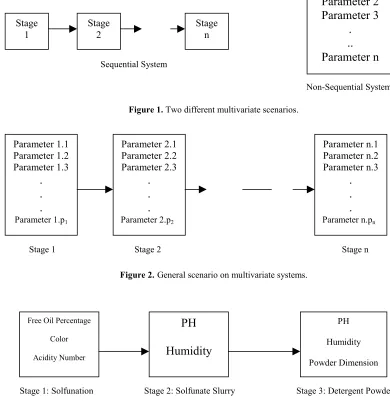
Sequential System
Non-Sequential System Figure 1. Two different multivariate scenarios.
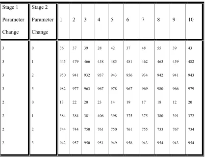
Stage 1 Stage 2 Stage n Figure 2. General scenario on multivariate systems.
Stage 1: Solfunation Stage 2: Solfunate Slurry Stage 3: Detergent Powder Figure 3. Three stages of detergent production line and their corresponding quality.
includes several serial stages as a sequential system. Sequential and non-sequential systems are graphically presented in Figure 1. In the sequential case, production lines have several stages and the quality of the product in each stage depends not only on the process of the current stage, but also on the quality of the input to the current stage, which is the output of the previous stage. Chemical industry is a good example of this case. In the non-sequential case, where there are several correlated
where the process has gone “out-of-control” and which of the variable(s) is (are) the cause of deterioration. A general scenario depicted in Figure 2 can be a system, which contains both of these categories.
The detergent production industry is a good example of these systems. Detergent production is a chemical-physical process, which in different stages of the process, different materials mix together and go through chemical reactions. This is Stage
1
Stage 2
Stage n
Parameter 1
Parameter 2
Parameter 3
.
..
Parameter n
Parameter 1.1 Parameter 1.2 Parameter 1.3
.
.
.
Parameter 1.p1Parameter 2.1 Parameter 2.2 Parameter 2.3
.
.
.
Parameter 2.p2Parameter n.1 Parameter n.2 Parameter n.3
.
.
.
Parameter n.pnFree Oil Percentage
Color
Acidity Number
PH
Humidity
PH
Humidity
systems have several stages in production; and in each stage of the production several correlated quality characteristics are present and used to control the process. Figure 3 shows the main stage of production and quality characteristics at each stage. The output quality of the second stage depends on the process of the first stage as well as the quality of sulfunic acid, which is the output of the first stage. We will use the data of stage one and stage two of such a system in example one. In the MVMSQC method, Niaki and Moeinzadeh [2] developed a statistic and an algorithm for the cause-selecting problem in which the population parameters are not known and are to be estimated. They also applied the Hotelling T2 statistic (Hotelling [3], Montgomery [4] or Ryan [5]) and regression concept to develop a criterion to eliminate the effect of the prior stage from the current stage’s quality characteristics. They suggested a statistical quality control system to address the general scenario by answering the following questions:
1. Is the process at each stage “in control”?
2. If the process of stage (i) is out-of-control, which characteristic(s) is (are) the cause of deterioration?
1. If the process shows an “out-of-control” signal in stages i and i+1, how has the output of stage i affected the result of stage i+1?
To address the first question they used the well-known Hotelling T2 statistics, then they applied the discriminant analysis to address the second question; and an iterative algorithm was developed to test each variable and subset of variables. In their research, the third question was answered by applying T2 statistic and regression concepts. They developed a criterion to eliminate the effect of the prior stage from the quality characteristics of the current stage.
The purpose of this research is to enhance the theoretical aspects of the MVMSQC method, to clarify its applications as well as to evaluate its
performance through series of simulated data and average run length studies.
LITERATURE REVIEW
The literature in Multivariate Quality Control can be classified into two broad categories; Sequential and Non-Sequential. The distinction between sequential and non-sequential processes is not in the order of occurrence of the processes, but in the order of measurement of the process parameters. Sequential Process The control of sequential processes is less of a problem since a change in a parameter affects only the upstream processes and does not affect the preceding processes. Using least-square regression seems to be the best possible solution to the problem (Mandel [6]). See also Zhang [7-10]. Constable et al. [11,12], Wade and Woodall [13] and Hawkins [14,15].
Zhang [7] has studied a system with several production stages in which each stage consists of one quality characteristic. The other approach, which was put forward by Mason et al. [16], has proposed an effective method to address sequential systems using double decomposition of Hotelling T2. In this model each stage can have more than one variable. This method is designed to detect stepwise changes. One draw back of this method is its excessive computation, especially when the number of time periods increases. Each time period adds one row and one column to the variance-covariance matrix. The other draw back of this method is its limited generality, where the quality characteristics of all stages remain the same, which is not the case in many real situations.
“out-of-control”. He divided the complete set of variables into two subsets and then tried to determine which one of the subset caused the “out-of-control” signal. He used the difference between the full squared distance and the reduced squared distance as the test statistic. By doing a series of tests and continuously dividing the subset of the variables into smaller subsets, it is possible to determine the “out-of-control” quality characteristics.
An extension of Murphy’s [17] work is Chua and Montgomery [18]. They proposed a three steps quality control process by using a Multivariate Exponential Weighted Moving Average (MEWMA) control chart, a backward selection algorithm and a hyper plane method. A MEWMA control chart is established after every new observation in a continuous basis until an “out-of-control” signal appears. If an “out-of-“out-of-control” signal appears, then the backward selection algorithm and the hyper plane method are used to diagnose it. An obvious draw back of this method is that it does not allow us to see trends, so it is not diagnostic on a continuous basis. This method does not necessarily always pinpoint the “out-of-control” quality characteristic. The method also uses only the MEWMA chart to detect initial “out-of-control” signals, which sometimes take a considerable amount of time to show up because of the inertia problem in the MEWMA chart. The MEWMA should always be used in conjunction with the Hotelling T2 (Lowry et. al. [19]).
The principal component analysis is a way of explaining the variance-covariance structure in a multivariate environment by the use of few linear combinations of the original variables. Jackson [20-23] gave a detailed description of principal components and its possible use as a multivariate quality control tool. Chang [24] extended Jackson’s work by giving a thumb rule to identify the cause of shifting in the overall mean based on unique distribution patterns exhibited by the
principal component charts. The problem with principal component is that they are not easily interpretable in many cases. They do not have a one-to-one relation with the original variables (i.e. the first principal component signaling does not mean that the first variable is “out-of-control”). Regardless of the order of variables, the principal components remain the same, so it is not possible to pinpoint a cause based on principal components. In some cases principal components can be very useful, depending on the context, but these successes cannot be generalized in all cases.
In order to diagnose the “out-of-control” variable in a non-sequential case, Alt [25] proposed an application of Bonferroni inequality to develop control charts. The control limits of these charts are wide and they are not effective when the shifts are small. We tried control limits based on simultaneous T2 intervals (Johnson and Wichern [26]), which were even wider than the control limits when using Bonferroni intervals.
Daganaskoy et. al. [27] proposed the use of univariate t-statistic for ranking the variables most likely to have changed. Then to further strengthen the belief that a certain variable has changed they applied Bonferroni type interval. The obvious draw back of this method is that it only tells you which variable is most likely to have shifted and this it is not conclusive. This method does not also allow us to study trends.
THE MVMSQC METHOD
In the MVMSQC procedure, it is assumed that the process at each stage of production possesses a multivariate normal distribution with unknown parameters (µ , Σ ), and Σ is constant during the study. The procedure consisted of four phases, in each of them the estimated value of (µ , Σ ) was used.
In phase zero, named the “Collecting Data for the Model Setup phase”, assuming an in control process, k groups of sample data were collected; each consisting n observations, and Xijm was defined to be the observation of the mth sample of parameter i in the jth group. Then the p*k sample means of parameters in k groups were computed as: (1) p 1,..., i , k 1,..., j ; 1
1 = =
= = n m ijm ij X n X
The overall sample mean of the ith parameter and the sample mean vector was calculated as:
(2) p , 1,... i ; k 1 j ij X k 1 i
X ∑ =
= = and (3) T p X , ... , 2 X , 1 X X =
The estimated element of row i and column j of the pooled sample variance-covariance matrix (SP) of the sample vector mean of the
p parameters, was then computed as:
(4) ) X -X )( X -X ( ) 1 k ( k 1 S S k 1 m j jm i im p
pij ji
∑
=
− = =
where i and j are equal to 1, 2, … , and p. To make sure that the setup phase had been successfully
completed, for each of the k groups Tj2 was calculated as: (5) ) X X ( S ) X X ( n
T 1 (j)
p ) j ( 2
j = − − −
and compared it against the Upper Control Limit (UCL) as: (6) F ) ) 1 p k kn p np kp knp (
UCL α(p,kn−k−p+1)
+ − − + − − =
whereX(j) denoted a vector with p elements that contained the group averages for each of the p parameters. If the values of Tj2 in all of the k groups did not exceed the UCL, then Tj2 values of stage s+1 were regressed on the Tj2 values of stage s and the regression parameters were estimated for future use. Otherwise, if any of the Tj2 exceeded the UCL, then the corresponding group(s) was investigated. Furthermore, if there was any assignable cause in them, the corresponding entire group(s) was eliminated and the computations were made again.
In phase one of the MVMSQC procedure, named the “Detecting Departure at Each Stage phase”, the actual behavior of stages of the production line was controlled through the Hotelling T2 statistic. If an “out-of-control” signal was detected for a group, the phase two of the procedure was then activated to find the parameter(s) causing the deviation. Also, if both of the subsequent stages were “out-of-control’, phase three of the method were activated to see whether the latter stage was “out-of-control” or if the former stage had been “out-of-control” and caused an “out-of-control” signal for the current stage.
causing the deterioration is (are) detected. The users of any multivariate system can find the technical reason of “out-of-control” signal much easier if they know which variable(s) is (are) the cause of deviation. Because of the statistical concerns, a cause selecting procedure must have the following three characteristics to be useful in real world application.
• It must be easy to use. This means that the interpretation of the results does not need a high level statistical expertise. An example of this, which does not satisfy this criterion, is using principal components for the Cause Selecting problem. The final results of the analysis consist of a set of independent variables none of which individually represents any of the original variables.
• The result must be straightforward. This means that the result should have a unique and unambiguous interpretation. Graphical methods addressed by Anderson [29], Andrews [30], Chamber et. al. [31], Chernoff [32], and Scott [33], have this draw back because they present the overall status of samples and this status can be assessed in different ways.
• In real world problems the values of the population parameters are rarely available. Therefore a test procedure must use the estimated values of the parameters.
EVALUATION OF PHASE THREE
In phase three of the MVMSQC algorithm, named the “Detecting the out-of-control stage”, a sequential multivariate problem was addressed. In this phase, the intuition of Zhang’s [10] method in univariate case was used and extended to a multivariate situation. Zhang has used the residual of observed value of a univariate quality characteristic with its regressed value on the
corresponding observation of the previous stage. Several statistics can be chosen for applying this idea on multivariate case. In MVMSQC method, Hotelling T2 was selected for two reasons. First, the quadratic form of Hotelling T2 magnifies the effect of any deviation and makes the test more sensitive. Second, the Hotelling T2 was applied in phase 1 of the procedure, and by using it in this phase there was no need for any extra calculation.
In MVMSQC procedure, several regression models are needed to be tested to find the best linear or non-linear regression model between Hotelling T2 of the current stage and Hotelling T2 of the previous stage, and there was no best general model. In this phase, instead of testing the observed value of Hotelling T2, the residuals of the observed value and the predicted value of Hotelling T2 were tested. If the process in stage s+1 is “in control” the residual will be a small value close to zero (positive or negative). Because if the system behaves as it did in phase zero of the procedure, the observed and the predicted values of Hotelling T2 will be close to each other. By a simple transformation, these residuals would have a “t” distribution, which can be used for establishing a test of hypothesis.
regression model.
Example 1: Consider the detergent production problem depicted in Figure 3. As the figure shows, there are three main stages in the production of detergent powder. In this example stage 1 and stage 2 of the production will be considered. Due to proprietary, we are unable to provide any more information about the nature of our data or specifics of possible signals. This was a consulting work done with the full understanding that no more than what we have stated here will be made public. However, we have used the desired values of the quality characteristic means and variance (by using the specification limit)* and the correlation among the quality characteristics (by interviewing an expert in the production line) for simulating data. *Management of the company claims that a natural tolerance limits (NTL) of their production is narrower than specification limits in standard. By relying on this statement, a PCR (Process Capability Ratio) of equal to one for each characteristic was assumed. Knowing that they are adjusting the process at the center of NTL, the standard deviation of each of the variables was then calculated.
Stage one of the production has a multi-normal distribution with µ= [67.5,12,97] and
For simulating the variables of stage 2, we have used the following relations:
where x21and x22 are the simulated variables of the
second stage with µ21=100 and µ22=150. Also x11 and x12 are the observed values of the variables in the first stage with their corresponding means µ11 and µ12, and finally ε1 and ε2 are normal random variables with mean equal to zero and a variance equal to the variance of their corresponding variables.
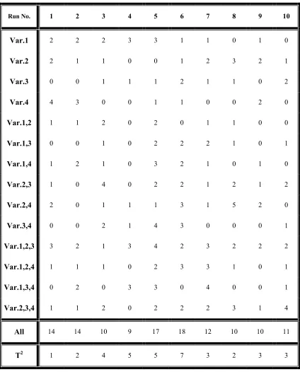
The distribution of TD (the statistic for testing the hypothesis that either the current stage or the previous stage is “out-of-control”) is not available. So simulation technique has been used to choose an appropriate value of UCL. One thousand data sets have been used to estimate the coefficients of the regression model. To specify the control limits for run time phase, the maximum value and the histogram of TD under different scenarios have been used. Table 1 shows the maximum values of TD under different scenarios and Charts 1 and 2 are two samples of the charts, which have been used to choose the UCL value.
After several trial and error studies we have chosen UCL to be equal to 5 and used it for the run time sets. Table 2 shows the number of “out-of-control” signals in 10 replications of 1000 observations for each scenario. The first column of Table 2 shows the amount of shift (in multiple of
σ) in the first variable of stage 1 and the second column shows the amount of shift (in multiple of
σ) in the first variable of the second stage. Each cell of Table 2 shows the number of “out-of-control” signals in 1000 observations for the corresponding replication of each scenario. The first and the fifth rows show the number of false alarms of the procedure which can be used to calculate the type I error of this phase. In univariate and one stage multivariate quality control for a specific statistic and control limits, type I error has a specific value. However, in the proposed multistage procedure, it is not correct. To clarify this statement, let’s restate the definition of type I error in this case. Type I error is the probability of having an “out-of-control” signal for
0.03
0.1 − 0.07 −
0.1 − 1.00 0.36
0.07 − 0.36 0.68 =
2
2
Σ
(7)
)
(
and
)
(
11 22 1211 21
21 2
12 22
1
=
+
+
=
ε
µ
µ
ε
µ
µ
x
x
x
the current stage when it is in control assuming the previous stage is “out-of-control”. In this case the probability of type I error depends not only on the control limits of the current stage control chart, but also on how the previous stage has been “out-of-control”.
As a second example the first and the fifth rows of Table 2 show this fact. In both rows, the current stage has not shifted, but the previous stage has been shifted equal to 3σ at the first row and 2σ at the second row. The numbers of false alarms are significantly different in these rows. As Table 2 indicates, TD is very sensitive when the mean of the current stage shifted 3σ (about 96%) regardless
of the amount of shift in the previous stage (rows 4 and 8). At 2σ shift in the mean of the current stage the procedure is very sensitive when the previous stage has shifted 3σ (about 94%). However, when both stages are shifted about 2σ, the sensitivity of the procedure goes down to 75%.
It should be mentioned that phase 3 of the procedure has been adjusted for our specific problem and the results can be used directly for other cases. However, we believe this approach can be modified for a wide range of real problems. The other point of phase three is used for simulation to find the critical value for the test, instead of being faced with the mathematical and pure statistical problems.
TABLE 1. The Maximum of TD in 1000 Data Sets Under Different Scenarios.
Scenario
µ
12Æ
3σ
µ
21Æ
0
σ
µ
12Æ
3
σ
µ
21Æ
3
σ
µ
12Æ
2
σ
µ
21Æ
0
σ
µ
12Æ
2
σ
µ
21Æ
1
σ
µ
12Æ
2
σ
µ
21Æ
2
σ
µ
12Æ
2
σ
µ
21Æ
3
σ
Max Value
of TD 11.2 89.5 8.6 48.5 61.9 86.2
Chart 1. The distribution of TD (the first variables of both
stages are shifted 3σ Number of rejected groups considering UCL=5 in 1000 observations is 999.
Chart 2. The distribution of TD (the first variables of both
TABLE 2. Number of “Out-of-Control” Signals in 1000 Observations. Stage 1 Parameter Change Stage 2 Parameter Change
1 2 3 4 5 6 7 8 9 10
3 3 3 3 2 2 2 2 0 1 2 3 0 1 2 3 36 445 950 982 13 384 744 942 37 479 941 977 22 384 744 957 39 466 932 963 20 381 750 950 28 458 937 967 23 406 761 951 42 485 943 978 14 398 750 949 37 481 956 967 19 375 761 958 48 462 934 969 17 375 755 943 55 463 942 980 18 380 733 954 39 459 941 966 12 391 767 943 43 482 943 979 20 372 734 954
AVERAGE RUN LENGTH STUDIES
In-Control ARL (Type I error) Why does the procedure use Hotelling T2 test in phase one, and why does it use the cause selecting method just for “out-of-control” groups? Average run length study for “in control” and “out-of-control” situations, is one of the most effective criteria to assess the capability of a procedure.
Assume that phase two of the procedure would have been used for each observed subgroup regardless of the results of phase one. If we consider a type one error equal to α for each test for each subset of variable(s) in the procedure, because of the repetitive nature of the procedure, the overall type one error of the procedure would
be higher than the basic value of α. A conservative type one error of the procedure in phase two can be achieved by assuming that all of the tests in different steps of the procedure are independent. If
αT gives this upper limit for the total type one error of phase two of the procedure, then:
However, because of the inherent dependency among the tests, the probability of the statistic plot inside the control limits is higher than 1-αT . To estimate the real values of type one and type two errors, one set of 200 subgroups with 6 samples in each subgroup of four-dimensional simulated multivariate normal variables with the
(8) ) 1 ( 1 1
∑
=− − = n i n i T α Cfollowing parameters has been used for the setup phase.
Then 10 replications of 1000 subgroups with 6 samples in each subgroup of four-dimensional simulated multivariate normal variables with the same parameters have been used as runtime subgroups for the simulation.
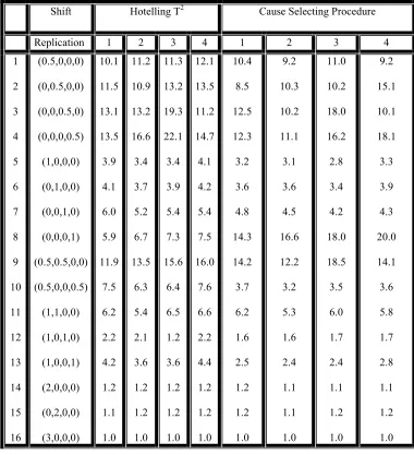
Using the setup data we have estimated these parameters and have used the estimated values for the rest of the simulation study. Table 3 shows the number of “out-of-control” signals in test of each subset of variables for 10 replications of 1000 groups. The last two rows of Table 3 show the total number of false alarms by the Hotelling T2 and cause selecting procedure respectively. A comparison of the results in these two rows reveals that the number of false alarms at the cause selecting procedure is significantly higher than the number of false alarms of Hotelling T2. This draw back can be managed by one of the following ways:
• Before using the procedure, estimate the real value of total type one error by using simulation. This means the user must set the value of type one error of each test in a way that the total type one error becomes equal to a desired α.
• Use phase two of the procedure only after you find out the system is “out-of-control” by applying another statistical test; this method has been chosen for this research, because we only apply cause selecting procedure if Hotelling T2 detects an “out-of-control” signal.
Out-Of-Control ARL (Type two error): In multivariate quality control, assessment of type
two error is not as straightforward as it is in the univariate case. This is because the level of shift is not the only factor in determining the type two error, but is also dependent on the correlation between parameters. A procedure can be sensitive in detecting a shift on one of the variables for specific amount of shift but insensitive in detecting the same level of shift in other variables. This phenomenon makes it impossible to benchmark different multivariate procedures. In general, there is no uniformly most powerful test available. However, before a procedure is used for monitoring a system, it must be tested for the important possible shifts and be evaluated in detecting these shifts. In this research different scenarios for different levels of shift in different subsets of the variables have been simulated. In this simulation study, we have used the same covariance structure under different mean shifts. The simulation study has made in two different ways. Table 4 summarizes the results of the first study, in which four replications of different scenarios with α=0.05 are used in Hotelling T2 as well as the cause selecting procedure. The results of this study shows that the MVMSQC procedure is very sensitive in detecting shifts (in multiple σ) in mean of equal or higher than 2σ (the last three rows of the table). For smaller shifts the sensitivity of the procedure depends on the structure of the variance-covariance matrix. As an example, consider rows five through eight, where at each row, one of the variable’s mean has been shifted by 1 σ. However, the sensitivity of the procedure is much higher in the first three rows; this can be explained by the existing lower correlation of the fourth variable with the other variables. Another interesting point is that the procedure is more sensitive for the shift in the mean of one variable than the shift in the mean of two variables. To investigate this point, consider rows one, two and nine. The ARL in rows one and two is lower than the ARL in row nine. Assuming µ=(0,0,0,0) and a
[
]
1.00
0.50
0.45
0.40
0.50
1.00
0.65
0.55
0.45
0.65
1.00
0.80
0.40
0.55
0.80
1.00
=
Σ
0,0,0,0
=
and
TABLE 3. In Control ARL (The No. of False Alarms in Test of 1000 Subgroups (αααα=0.01)).
Run No. 1 2 3 4 5 6 7 8 9 10
Var.1 2 2 2 3 3 1 1 0 1 0
Var.2 2 1 1 0 0 1 2 3 2 1
Var.3 0 0 1 1 1 2 1 1 0 2
Var.4 4 3 0 0 1 1 0 0 2 0
Var.1,2 1 1 2 0 2 0 1 1 0 0
Var.1,3 0 0 1 0 2 2 2 1 0 1
Var.1,4 1 2 1 0 3 2 1 0 1 0
Var.2,3 1 0 4 0 2 2 1 2 1 2
Var.2,4 2 0 1 1 1 3 1 5 2 0
Var.3,4 0 0 2 1 4 3 0 0 0 1
Var.1,2,3 3 2 1 3 4 2 3 2 2 2
Var.1,2,4 1 1 1 0 2 3 3 1 0 1
Var.1,3,4 0 2 0 3 3 0 4 0 0 1
Var.2,3,4 1 1 2 0 2 2 2 3 1 4
All 14 14 10 9 17 18 12 10 10 11
T2 1 2 4 5 5 7 3 2 3 3
high positive correlation between the first two
variables, this can be explained by the higher
probability to get a point around (0.5, 0.5, 0, 0)
sensitive as Hotelling T
2test, while it can also
detect the variable(s) causing deterioration.
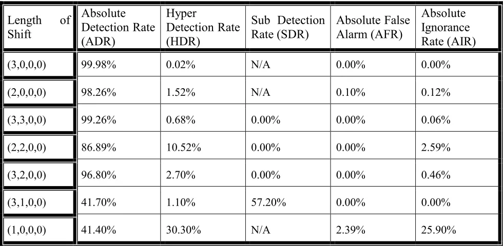
In the second simulation study, to show the effectiveness of the procedure more clearly, we have defined the following terms and have used them in Table 5 to better explain the results:• Absolute Detection Rate (ADR): The percentage of parameters that are “out-of-control” and are detected as such.
• Hyper-Detection Rate (HDR): The percentage
of times the procedure has detected the “out-of-control” variable(s), but another in control variable is also signaled as being “out-of-control”.
• Sub-Detection Rate (SDR): The percentage of times the procedure has detected only a subset of the “out-of-control” variables.
• Hyper-Detection Rate (HDR): The percentage of times the procedure has detected the “out-of-control” variable(s), but another in control variable is also signaled as being “out-of-control”.
TABLE 4. Comparisons of Hotelling T2 and Cause Selecting Procedure Out-Of-Control ARL (
α αα α=0.05).
Shift Hotelling T2 Cause Selecting Procedure
Replication 1 2 3 4 1 2 3 4
• Absolute False Alarm Rate (AFR): The percentage of times the procedure shows a variable or a subset of variables to be “out-of-control”, when none is “out-of-control”.
Absolute Ignorance Rate (AIR): The percentage of times the procedure does not show a variable or a subset of variables to be “out-of-control”, when at least one is “out-of-control”.
This categorization is important because the critical situations are different in industries. If the cost of type one error or examination of an “out-of-control” signal is very high, the user should consider the HDR to be as important as AFR. On the other hand, if the cost of type two error or ignorance of an “out-of-control” variable is very high, SDR must be considered to be as important as AFR in evaluating the procedure. Ideally ADR can lead to find the cause of “out-of-control” signal; however, in some cases, HDR or SDR also can be a good starting point in looking for the root
of the problem because they provide more information than Hotelling T2 does.
Table 5 shows the average of the above rates, which is resulted from 10 replications of each scenario. Review of Table 5 shows the results clearly. As rows 1-5 show, when one or two variables have been shifted by 2 or more σ, the procedure is very sensitive. When one variable shifts 3σ and the other variable shifts 1σ (row 6), the procedure faces a high SDR (57.2%). This is because the contribution of the first variable in the value inflation of the statistic is much more than the other variable and this covers the effect of the other variable in the value of the statistic.
On the other hand, the last row of Table 4 shows that the sensitivity of the procedure goes down for changes around 1σ and it has a high amount of HDR (30.3%) and AIR (25.9%). This means that the procedure is not effective for shifts of small magnitude.
TABLE 5. The Average of Error Rates Resulting from 10 Replications of Each Scenario.
Length of
Shift
Absolute
Detection Rate
(ADR)
Hyper
Detection Rate
(HDR)
Sub Detection
Rate (SDR)
Absolute False
Alarm (AFR)
Absolute
Ignorance
Rate (AIR)
(3,0,0,0) 99.98% 0.02% N/A 0.00% 0.00%
(2,0,0,0) 98.26% 1.52% N/A 0.10% 0.12%
(3,3,0,0) 99.26% 0.68% 0.00% 0.00% 0.06%
(2,2,0,0) 86.89% 10.52% 0.00% 0.00% 2.59%
(3,2,0,0) 96.80% 2.70% 0.00% 0.00% 0.46%
(3,1,0,0) 41.70% 1.10% 57.20% 0.00% 0.00%
CONCLUSION AND FURTHER WORK
We have presented the practical aspects of the MVMSQC method to control a multivariate-multistage production system. In this research, the cause-selecting phase (phase three) of the MVMSQC algorithm has been theoretically enhanced and a numerical example has been given to clarify and evaluate the performance of this phase. We have considered a linear relation among the variables of two stages and we believe that phase three of the procedure is a good area for the future work.
Even though the procedure works effectively on our detergent production example, there is no guarantee that the linear relation will work for every system. At this point it is the user’s responsibility to find the best linear or non-linear relation between the Hotelling T2 of any consecutive stages. Also the performance of the procedure has been evaluated through several simulation studies. Results show that while the procedure works well for large amount of shifts in the mean of the parameters in consecutive stages, it has some drawbacks for small shifts.
REFERENCES
1. Montgomery, D. C., "Introduction to Statistical Quality Control", John Wiley and Sons, New York, (1991). 2. Niaki, S. T. and Moeinzadeh, B., "A Multivariate Quality
Control Procedure in Multistage Production Systems",
International Journal of Engineering, Vol. 10, No. 4, (1997).
3. Hotelling, H., "Multivariate Quality Control, Techniques of Statistical Analysis", (C. Eisenhart, M. W. Hastay, and W. A. Wallis Eds.), McGraw-Hill, New York, (1947). 4. Montgomery, D. C., "Introduction to Statistical Quality
Control", 3rd Ed., John Wiley and Sons, New York,
(1996).
5. Ryan, T. P., "Statistical Methods for Quality Improvement", John Wiley and Sons, New York, (1989). 6. Mandel, B. J. "The Regression Control Chart", Journal of
Quality Technology, Vol. 1, No. 1, (1969).
7. Zhang, G. X., "A New Type of Control Charts and a Theory of Diagnosis with Control Charts", Proceedings of World Quality Congress Transactions, American
Society for Quality Control, (1984).
8. Zhang , G. X., "Brief Introduction to the Cause Selecting Theory", Economic Quality Control, Newsletter of the Wurzburg Research Group of Quality Control, Vol. 4, (1989).
9. Zhang, G., "A New Diagnosis Theory with Two Kinds of Quality", Total Quality Management, Vol. 1, No. 2, (1990).
10. Zhang, G. X., "Cause Selecting Control Charts and Diagnosis, Theory and Practice", Aarhus School of Business, Department of Total Quality Management, Aarhus, Denmark, (1992).
11. Constable, G. K., Clearly M. J. and Zhang, G., "Cause-Selecting Control Charts. A New Type of Quality Control Charts", ASQC Quality Congress Transactions, (1987). 12. Constable, G. K., Cleary, M. J., Tickel, C. and Zhang, G.,
"Use of Cause-Selecting Control Charts in the Auto Industry", ASQC Quality Congress Transactions, Dallas, (1988).
13. Wade, M. R. and Woodall, W. H., "A Review and Analysis of Cause-Selecting Control Charts", Journal of Quality Technology, Vol. 25, No. 3, (1993).
14. Hawkins, D. M., "Multivariate Quality Control Based on Regression – Adjusted Variables", Technometrics, Vol. 33, No. 1, (1991).
15. Hawkins, D. M., "Regression Adjusted for Variables in Multivariate Quality Control", Journal of Quality Technology, Vol. 25, No. 3, (1993).
16. Mason, R. L., Tracy, N. D. and Young, J. C., "Monitoring a Multivariate Step Process", Journal of Quality Technology, Vol. 28, (1996).
17. Murphy, B. J., "Selecting Out-Of-Control Variables with the T2 Multivariate Quality Control Procedure", The
Statistician, Vol. 36, (1987).
18. Chua, M. K. and Montgomery, D., "An Investigation and Characterization of a Control Scheme for Multivariate Quality Control Charts", Quality and Reliability Engineering International, Vol. 8, (1992).
19. Lowry, C. A., Woodall, W. H., Champ, C. W. and Rigdon, S. E., "A Multivariate Exponentially Weighted Moving Average Control Chart", Technometrics, Vol. 34, No. 1, (1992).
20. Jackson, J. E., "Quality Control Methods for Several Related Variables", Technometrics, Vol. 1, (1959). 21. Jackson, J. E., "Principal Component and Factor Analysis,
Part I – Principal Components", Journal of Quality Technology, Vol. 12, No. 4, (1980).
Quality Technology, Vol. 13, No. 2, (1981).
23. Jackson, J. E. and Morris, R. H., "An Application of Multivariate Quality Control to Photographic Processing",
Journal of the American Statistical Association, Vol. 52, (1957).
24. Chang, T., "Statistical Control of Correlated Variables",
ASQC Quality Congress Transactions, Milwaukee, (1991).
25. Alt, F. B., "Multivariate Quality Control", Encyclopedia of Statistical Science, Vol. 6 (S. Kotz and N. Johnson, Eds.), John Wiley and Sons, New York, (1985).
26. Johnson, R. A. and Wichern, D. W., "Applied Multivariate Statistical Analysis", 3rd ed., Prentice-Hall Inc.,
Englewood Cliffs, N.J., (1992).
27. Doganaksoy, N., Faltin, F. W. and Tucker, W. T., "Identification of Out-Of-Control Quality Characteristics in a Multivariate Manufacturing Environment",
Communications in Statistics – Theory and Methods,
Vol. 20, (1991).
28. Mason, R. L., Tracy, N. D. and J. C. Young, "Decomposition of T2 for Multivariate Control Chart
Interpretation", Journal of Quality Technology, Vol. 27, (1995).
29. Anderson, E., "A Semigraphical Method for the Analysis of Complex Problem", Technometrics, Vol. 2, (1960). 30. Andrews, D. F., "Plots of High-Dimensional Data",
Biometrics, Vol. 28, (1972).
31. Chamber, J. S., Cleveland, W. S., Kleiner, B. and Tukey, P. A., "Graphical Methods for Data Analysis", Wadsworth Publishing Co., Inc., Belmont, CA, (1983).
32. Chernoff, H., "The Use of Faces to Represent Points in K-Dimensional Space Graphically", Journal of American Statistical Association, Vol. 74, (1973).