Please cite this article as: Y. Karimi, S. Rashahmadi, R. Hasanzadeh,The Effects of Newmark Method Parameters on Errors in Dynamic Extended Finite Element Method Using Response Surface Method,International Journal of Engineering (IJE),IJE TRANSACTIONS A: Basics Vol. 31, No. 1, (January 2018) 50-57
International Journal of Engineering
J o u r n a l H o m e p a g e : w w w . i j e . i rThe Effects of Newmark Method Parameters on Errors in Dynamic Extended Finite
Element Method Using Response Surface Method
Y. Karimi, S. Rashahmadi*, R. Hasanzadeh
Mechanical Engineering Department, Urmia University, Urmia, Iran
P A P E R I N F O
Paper history:
Received 17September2016
Received in revised form 22August2017 Accepted 02December2017
Keywords: Dynamic XFEM Time Integration Newmark Method Response Surface Method Error
A B S T R A C T
The Newmark method is an effective method for numerical time integration in dynamic problems. The results of Newmark method are function of its parameters (β, γ and ∆t). In this paper, a stationary mode I dynamic crack problem is coded in extended finite element method )XFEM( framework in Matlab software and results are verified with analytical solution. This paper focuses on effects of main parameters in Newmark method for dynamic XFEM problems. Also use of the response surface method (RSM) a regression model is presented for estimating error of dynamic stress intensity factors (DSIF) with high validity according to results of analysis of variance (ANOVA). This work enables one to understand the effect of Newmark parameters on error of DSIFs and to find optimum β and γ for a determined number of time steps (N). This procedure is highly effective in order to manage the computational cost and enhance the accuracy at the desired domain. The effect of the considered parameters on error, is investigated using RSM in Minitab software and optimum state for minimization of errors is illustrated.
doi: 10.5829/ije.2018.31.01a.08
NOMENCLATURE dyn
I
K Mode I dynamic stress intensity factor Greek Symbols
dyn II
K Mode II dynamic stress intensity factor 0 Applied stress (MPa)
c
t The time when applied stress wave reaches the crack tip for the first time (s) Density (kg/m3) t
Time step (s) Poission’s ratio
3c
N t t Number of time steps Parameter of Newmark method
1
E Error of dynamic stress intensity factors in a vicinity of time tc(%) Parameter of Newmark method 2
E Error of dynamic stress intensity factors in a vicinity of time 3tc(%) Superscripts d
C Dilatational wave speed ( m/s) aux Auxiliary fields
( )
H x Heaviside or jump function dyn Dynamic
l
F Singular or asymptotic enrichment functions Subscripts
E Young modulus of elastisity (GPa) in Interaction
1. INTRODUCTION1
Dynamic problems consist of a wide range of engineering problems in various fields [1, 2]. Finite element method is one of interesting numerical methods
*Corresponding Author’s Email: [email protected] (S. Rashahmadi)
Mohammadi [9] developed dynamic XFEM for analysis of composites. It is mandatory to select an accurate time integration algorithm in simulation of a dynamic problem. Time integration methods include the explicit and implicit approaches with different complexity, speed, efficiency and accuracy. Explicit approach is simple and fast, but it is less accurate and suffers from stability conditions. Implicit approaches are more accurate and stable, but they are computationally more expensive [9]. In wave propagation studies, small time steps must be used in order to represent the nature of problem. Therefore, very small time increments must be used, which usually enhances computation costs [10]. Implicit methods need a balance between the accuracy
and the computation time [11]. Alamatian
[12]introduced implicit multi time step integration on dynamic analyses with constant time step. Alamatian [13] presented an implicit time integration method with higher order accuracy for dynamic problems. Shojaee et al. [14] studied on an implicit time integration method which its advantage is eliminating conditional stability. The results of Newmark method are function of its parameters (β, γ and ∆t). Stability of results depends on values of β, γ and their accuracy depends on values of β,
γ and time increment (∆t). The computation time is only depend on ∆t. A huge part of errors in dynamic XFEM problems are errors due to time integration method. Control and mangement of these errors is an important challenge. Analytical solution of benchmark problems which usually used to verify numerical approaches, are based on semi-infinite or infinite plate assumption. In order to remove the effect of reflected stress wave on the crack tip, the numerical simulation of finite plates is perfomed until the reflected dilatational wave from another edge of the plate reaches the crack tip. The highest errors of dynamic stress intensity factors occur when:
1. Initial stress wave reaches the crack tip, which highest error in a vicinity of this time is called E1 in the present work.
2. Reflected wave from the end of the plate reaches the crack tip, and most error in a vicinity of this time is called E2.
In this paper a new look at Newmark method from statistical point of view is demonstrated. The aim of this study is to determine the effects of parameters of Newmark method (i.e. β, γ and N) on the errors E1 and
E2. A dynamic fracture mechanics problem in the framework of XFEM using the response surface methodology (RSM) was studied. In addition, regression models for errors E1 and E2 are presented.
2. GOVERNING EQUATION AND FORMULATION
2.1. Basics of XFEM Extended finite element
method is based on enrichment of displacement field. In XFEM, finite element mesh is produced regardless of existence and location of discontinuity. Nodes around discontinuity are selected to be enriched; thus, some additional degrees of freedom are added to classical finite element at selected nodes due to enrichment of displacement field. The displacement field for a domain containing discontinuity is exprssed as Equation (1) [3, 5]:
4
1
h
i i j j
i I j J
k
k l l
k K l
u x x u H x x a
x b F x
(1)In which I is the set of total nodes, J is the set of red squared nodes and K is the set of blue circled nodes as shown in Figure 1. H(x) is Heaviside or jump function and used for nodes of completely cut elements:
1 1above the crack H x
below the crack
(2)
The functions
l
F x (l1, 2,3, 4)are the crack tip enrichment functions and are defined as:
sin( / 2), cos( / 2), ,
sin( / 2) sin , cos( / 2) sin l
r r
F r
r r
(3)
where r and θ are the polar coordinates in the local crack tip coordinate system.
In XFEM implementation two points must be considered:
1. Using Equation (1), at node xi will have u x
i ui which is a contradiction. A simple idea to solve this matter is shifting enrichment functions:
4
1
h
i i j j j
i I j J
k
k l l l k
k K l
u x x u H x H x x a
x b F x F x
(4)2. Shared nodes between completely cut elements and crack tip elements must be enriched only by crack tip enrichment functions.
2.2. XFEM Dynamic Equation of Motion The weak form of momentum equation of the initial/boundary value problem for a body with traction-free crack Γc shown in Figure 2 stated as follows:
. . .
t
u ud d t ud
(5)The discretized form of Equation (5) in framework of XFEM ignoring damping effects would be given as follows:
h
h
M u K u F (6)
The mass matrix M, stiffness matrix K, external load vector F and nodal degrees of freedom u for an element, respectively are defined as follows:
M M M
M = M M M
M M M
uu ua ub ij ij ij
e au aa ab
ij ij ij ij
bu ba bb ij ij ij
(7)
K K K
K = K K K
K K K
uu ua ub ij ij ij
e au aa ab
ij ij ij ij
bu ba bb ij ij ij
(8)
F = F , F , Fie iu ia ib T (9)
u =h , , T
u a b (10)
The components of mass matrix, stiffness matrix and force vector, respectively are given as follows:
( ) ( ) d
e
T
ij i j
M h N N
, u a b, ,
(11)(B ) C(B ) d
e
T
ij i j
K h
, u a b, ,
(12)( )T
i i
F N td
u a b, ,
(13)where matrices B and N for a four node element (i1, 2,3, 4)and using four asymptotic functions (l1, 2, 3, 4) are stated as Equations (14) to (19).
Figure 2. Initial configuration of domain
0 0 i u i i N N N
(14)
0 0 i a i i HN N HN
(15)
0 0 l i b i l i F N N F N
(16)
, , , , 0 0 i x u
i i y
i y i x N B N N N (17) , , , , 0 0 i x u
i i y
i y i x HN B HN HN HN (18) , , , , , , , , 0 0
l x i l i x u
i l y i l i y
l y i l i y l x i l i x F N F N
B F N F N
F N F N F N F N
(19)
2.3. Newmark Time Integration Method After
construction of matrices, the Newmark time integration algorithm is used to obtain nodal accelerations, velocities and displacements at each time step, respectively as below[15]:
1 1
2 1
2
1
( )
(1 2 ) 2
n n
n n
n
U tU
U M t K F K t
U (20)
1 (1 ) 1
n n n n
U U tU tU (21)
2
2
1 1 (1 2 ) 1
2
n n n n n
t
U U tU U t U
(22)
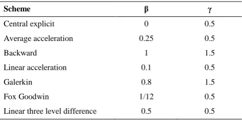
where,β and γ are constant parameters which accuracy and stability of numerical scheme depends on their values. Some of common numerical schemes with different values of β and γ has been reported in reference [16] as summarized in Table 1:
TABLE 1. Some of numerical schemes
Scheme β γ
Central explicit 0 0.5
Average acceleration 0.25 0.5
Backward 1 1.5
Linear acceleration 0.1 0.5
Galerkin 0.8 1.5
Fox Goodwin 1/12 0.5
In XFEM problems, central explicit and average acceleration (implicit mean acceleration) schemes were used [10, 17].
2.4. Stress Intensity Factors Computation
Interaction integral is derived via a two-field problem consisting of state 1, the actual field and state 2, the auxiliary field:
1 2 (1) (2) (1,2)
J J J I (23)
A simple to implementation way for calculation of dynamic stress intensity factors is the domain-independent form of interaction integral presented by Rethore [8]:
, ( , ) ( , , )
dyn aux aux aux aux
in k j ml m l l l kj ij i k ij i k A
I
q u u u u u dA, , , , ,
( aux aux) ( aux aux) k ij j i k i i k i i k i i k A
q u u u u u u u dA
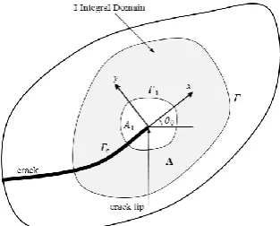
(24)The virtual extension field q is a smooth function tangent to the crack faces, varying from q=0 at the exterior boundary Γ at Figure 3 to q=1 near the crack tip.
The interaction integral is related to dynamic stress intensity factors in a plane strain condition as follows:
2
2(1 )
( )
in dyn aux dyn aux
I I II II
I K K K K
E
(25)
dyn I
K is evaluated by defining the auxiliary state as the pure mode I ( aux 1
I
K and aux 0 II
K ) and in a similar way, dyn
II
K can be obtained.
3. DESIGN OF EXPERIMENTS (DOE)
In order to optimize response variables in presence of various factors, design of experiments (DOE) was used. The most important objective in the DOE is to achieve the desired response with the lowest number of experiments [18].
Figure 3. The contour Γ and its interior area A
In this study, for optimization of process, investigation the regression model and finding the effect of variable parameters on the output, response surface method (RSM) was used.
The RSM regression model is generally quadratic full equation or reduced form of it is stated as Equation (26) [19]:
2
0 1 2 3
1 1
n n
i i i j
i i i j
y x x x x
(26)In Equation (26), y is the response variable,
0
, 1
, 2
and
3
are constant, linear, quadratic and interaction coefficients, respectively. Also xi and xj are the independent variables and
is the statistical error.After determining the regression model, efficiency of the model is checked using R2 as Equation (27) that can be obtained from analysis of variance (ANOVA) [20].
2
1 r
T
SS R
SS
(27)
where,
r
SS and
T
SS are the residual and total sum of squares, respectively.
In the present study, β, γ and N are considered as variable parameters and the effects of these parameters on the E1 and E2 are investigated using RSM. For selecting the range of parameters, range of time steps should be determined at first in order to manage camputational time, then by a few trial and error at upper and lower bound of N, range of β andγ could be determined so that the stability and error would be rational. For this purpose, by selecting the range of parameters, the design of experiments was performed according to the central composite design (CCD) with 20 experiments using Minitab software as summaraized in Table 2.
4. RESULTS AND DISCUSSION
The example considered for verifying codes is a finite plate with a stationary crack subject to a dynamic loading as shown in Figure 4. This example is a pure mode I problem ( dyn 0
II
K ). Analytical solution of this
problem is presented by Freund as stated in Equation (28) [21]:
0
0 ( ) 2 (1 2 )( )
1
c
I d c
c if t t
K t C t t
if t t
(28)
where
c d
t h C is the time when stress wave reaches the
(t3tc3h Cd) since the assumption of the analytical solution is infinite plate.
TABLE 2. The design of experiments according to RSM
Run Beta Gamma N
1 0.8549 0.5452 181
2 0.6295 0.5102 300
3 0.4041 0.4752 181
4 0.4041 0.4752 419
5 0.6295 0.5102 300
6 0.6295 0.5700 300
7 0.6295 0.5102 300
8 1.0000 0.5102 300
9 0.8549 0.4752 181
10 0.6295 0.4500 300
11 0.6295 0.5102 300
12 0.4041 0.5452 419
13 0.6295 0.5102 500
14 0.4041 0.5452 181
15 0.6295 0.5102 100
16 0.6295 0.5102 300
17 0.8549 0.5452 419
18 0.6295 0.5102 300
19 0.2500 0.5102 300
20 0.8549 0.4752 419
The dimensions are: L=10(m), a=5(m), h=2(m) and the material properties are the follows: Young’s modulus
211( )
E GPa , poisson’s ratio 0.3 and density
3
7800 (kg m)
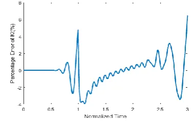
. The tensile stress applied on the top surface is 1(MPa). A 40×100 regular quadrilateral meshes was used. The time integration scheme used was implicit mean acceleration scheme with 250 time steps. The dynamic stress intensity factors obtained from code has a good agreement with analytical solution as shown in Figure 5. Percentage error is also given in Figure 6. The stress intensity factors are normalized by 0 h and
time is normalized by tc. According to Figure 6, the
most errors are at the vicinity of tNormalized1 when stress wave reaches the crack tip for the first time, and the vicinity of tNormalized 3 when the reflected stress wave reaches the crack tip [8].
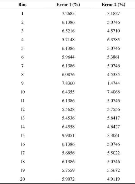
The results of twenty different experiments were obtained as presented in Table 3 using verified codes.
The result of normality test using SPSS software according to Kolmogorov-Smirnov method showed that P-values were equal to 0.067 and 0.293 (larger than statistical error i.e. 0.05) for E1 and E2, respectively. Therefore, the obtained results were followed normal distribution [22].
Figure 4. Geometry and loading for the dynamic problem
Figure 5. Comparison between normalized DSIF obtained from code and normalized analytical solution
Figure 6. Percentage error of I
K using 250 time steps,
0.25
and 0.5, are 1E 5% and E26.5%
The regression models for E1 and E2 were obtained using Minitab software; as expressed in Equations (29) and (30) respectively.
2 2 2
1 1.6 11.4 27.1 0.0272
2.59 27.0 0.000035
9.1 0.00844 0.0078
E N
N
N N
(29)
2 2 2
2 74.4 25.2 264 0.0421
3.51 243 0.000024 45.2 0.01322 0.0544
E N
N
N N
(30)
The results of ANOVA are summarized in Table 4 for
TABLE 3. The results of experiments
Run Error 1 (%) Error 2 (%)
1 7.2685 3.1827
2 6.1386 5.0746
3 6.5216 4.5710
4 5.7148 6.3785
5 6.1386 5.0746
6 5.9644 5.3861
7 6.1386 5.0746
8 6.0876 4.5335
9 7.8360 1.4744
10 6.4355 7.4068
11 6.1386 5.0746
12 5.5628 5.7556
13 5.4536 5.8417
14 6.4558 4.6427
15 9.9051 3.3061
16 6.1386 5.0746
17 5.6856 5.5022
18 6.1386 5.0746
19 5.7559 5.5672
20 5.9072 4.9119
TABLE 4. The results of ANOVA
Source Degree of freedom
P-value
E1 E2
Model 9 0.001 0.011
Linear 3 0.000 0.002
Square 3 0.008 0.137
Interaction 3 0.514 0.275
The P values less than 0.05, indicates that the desired parameters are effective [23]. It was observed that the linear and square terms were effective in the regression model of E1 while the square term was not effective in model of E2. Also the results indicated that obtained regression models have high efficiency for estimating error.
The main effect of parameters on E1 was obtained as illustrated in Figure 7. The results revealed that the E1
changed significantly with the change in the value of N. By increasing N, the E1 decreases markedly and the optimum value is in the range of 380-410 of N for minimum error. Also, the results illustrated that by increasing gamma, the E1 slightly decreases. As a
matter of fact, 0.57 is the best value for gamma for minimization of E1 in the considered range. Another result that could be obtained from Figure 7 is this fact that the optimum level for beta is 0.25 at which the minimum value of E1 was achieved.
Also, the main effect of parameters on E2 was achived as Figure 8. The results indicated that in contrary to E1, the E2 decreases as beta increases. The optimum value for gamma is 0.52 for minimization of
E2. Also, the results demonstrated that 100 is the best value for N at which E2 is minimumin.
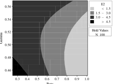
The interaction effect of beta and gamma on E1 is shown in Figure 9.
Figure 7. The main effect of parameters on E1
Figure 8. The main effect of parameters on E2
Figure 9. Interaction effect of beta*gamma on E1 when
N=100
0.9 0.6 0.3 9
8
7
6
5
0.55 0.50
0.45 100 300 500 Beta
E
1
Gamma N
0.9 0.6 0.3 6
5
4
3
2
0.55 0.50
0.45 100 300 500 Beta
E
2
Gamma N
N 100 Hold Values
Beta
G
a
m
m
a
1.0 0.9 0.8 0.7 0.6 0.5 0.4 0.3 0.56
0.54
0.52
0.50
0.48
0.46
The results demonstrate that in lowest values of beta, the E1 is in optimum state and is smaller than 8% for all values of gamma. Figure 10 shows the interaction effect of beta and gamma on E2. Figure 10 reveals that in the highest values of beta (beta>0.8), the E2 is minimum almost for all values of gamma. Also, the results indicated that in a constant value of gamma, the E2
decreases as beta increases.
Figure 10. Interaction effect of beta*gamma on E2 when
N=100
5. CONCLUDING REMARKS
In this study, the XFEM was implemented to model a dynamic problem with a stationary crack. Obtained dynamic stress intensity factors was verified with analytical solution. Also, the effects of parametes β, γ
and ∆t of the Newmark time integration method on the errors at two critical times was demonstrated. These errors are called E1 andE2 in this paper. The regression models were introduced for errors E1 and E2, which according to analysis of variance (ANOVA) results have high validity. The results showed that E1 has an inverse relation with γ and N and direct relation with β, while E2 has an inverse relation with β and the direct relation with N. Until 0.52 the relation between γ
and E2 is inverse and for greater values of γ, this relation is direct.
6. REFERENCES
1. Heidari, A. and Salajegheh, E., "Approximate dynamic analysis of structures for earthquake loading using fwt", International Journal of Engineering Transactions B Applications, Vol. 20, No. 1, (2007), 37-47.
2. Kaynia, A. and Dargush, G., "Fundamental solutions of dynamic poroelasticity and generalized termoelasticity", International Journal of Engineering, Vol. 5, No. 1&21, 1-10.
3. Belytschko, T. and Black, T., "Elastic crack growth in finite elements with minimal remeshing", International Journal for
Numerical Methods in Engineering, Vol. 45, No. 5, (1999), 601-620.
4. Armero, F. and Linder, C., "Numerical simulation of dynamic fracture using finite elements with embedded discontinuities",
International Journal of Fracture, Vol. 160, No. 2, (2009), 119-141.
5. Dolbow, J. and Belytschko, T., "A finite element method for crack growth without remeshing", International Journal for Numerical Methods in Engineering, Vol. 46, No. 1, (1999), 131-150.
6. Stolarska, M., Chopp, D., Moës, N. and Belytschko, T., "Modelling crack growth by level sets in the extended finite element method", International Journal for Numerical Methods in Engineering, Vol. 51, No. 8, (2001), 943-960.
7. Belytschko, T., Chen, H., Xu, J. and Zi, G., "Dynamic crack propagation based on loss of hyperbolicity and a new discontinuous enrichment", International Journal for Numerical Methods in Engineering, Vol. 58, No. 12, (2003), 1873-1905.
8. Réthoré, J., Gravouil, A. and Combescure, A., "An energy‐conserving scheme for dynamic crack growth using the extended finite element method", International Journal for Numerical Methods in Engineering, Vol. 63, No. 5, (2005), 631-659.
9. Mohammadi, S., "Xfem fracture analysis of composites, Wiley Online Library, (2012).
10. Menouillard, T., Rethore, J., Combescure, A. and Bung, H., "Efficient explicit time stepping for the extended finite element method (x‐fem)", International Journal for Numerical Methods in Engineering, Vol. 68, No. 9, (2006), 911-939.
11. Zhou, J. and Zhou, Y., "A new simple method of implicit time integration for dynamic problems of engineering structures",
Acta Mechanica Sinica, Vol. 23, No. 1, (2007), 91-99.
12. Alamatian, J., "A modified multi time step integration for dynamic analysis", International Journal of Engineering-Transactions B: Applications, Vol. 25, No. 4, (2012), 303-314.
13. Alamatian, J., "New implicit higher order time integration for dynamic analysis", Structural Engineering and Mechanics, Vol. 48, No. 5, (2013), 711-736.
14. Shojaee, S., Rostami, S. and Abbasi, A., "An unconditionally stable implicit time integration algorithm: Modified quartic b-spline method", Computers & Structures, Vol. 153, (2015), 98-111.
15. Newmark, N.M., "A method of computation for structural dynamics", Journal of the Engineering Mechanics Division, Vol. 85, No. 3, (1959), 67-94.
16. Zienkiewicz, O.C., "A new look at the newmark, houbolt and other time stepping formulas. A weighted residual approach",
Earthquake Engineering & Structural Dynamics, Vol. 5, No. 4, (1977), 413-418.
17. Liu, P., Bui, T., Zhang, C., Yu, T., Liu, G. and Golub, M., "The singular edge-based smoothed finite element method for stationary dynamic crack problems in 2d elastic solids",
Computer Methods in Applied Mechanics and Engineering, Vol. 233, No., (2012), 68-80.
18. Okafor, E.C., Ihueze, C.C. and Nwigbo, S., "Optimization of hardness strengths response of plantain fibers reinforced polyester matrix composites (PFRP) applying taguchi robust design", International Journal of Engineering, Vol. 26, No. 1, (2013), 1-11.
19. Alimirzaloo, V. and Modanloo, V., "Minimization of the sheet thinning in hydraulic deep drawing process using response surface methodology and finite element method", International Journal of Engineering (IJE), Transactions B: Applications, Vol. 29, No. 2, (2016), 264-273.
N 100 Hold Values
Beta
G
a
m
m
a
1.0 0.9 0.8 0.7 0.6 0.5 0.4 0.3 0.56
0.54
0.52
0.50
0.48
0.46
20. Nejad, S.J.H., Hasanzadeh, R., Doniavi, A. and Modanloo, V., "Finite element simulation analysis of laminated sheets in deep drawing process using response surface method", The International Journal of Advanced Manufacturing Technology, Vol. 93, No. 9-12, (2017), 3245-3259.
21. Freund, L.B., "Dynamic fracture mechanics, Cambridge university press, (1998).
22. Azdast, T., Hasanzadeh, R. and Moradian, M., "Optimization of process parameters in FSW of polymeric nanocomposites to
improve impact strength using step wise tool selection",
Materials and Manufacturing Processes, (2017), doi: 10.1080/10426914.2017.1339324.
23. Eungkee Lee, R., Afsari Ghazi, A., Azdast, T., Hasanzadeh, R. and Mamaghani Shishavan, S., "Tensile and hardness properties of polycarbonate nanocomposites in the presence of styrene maleic anhydride as compatibilizer", Advances in Polymer Technology, doi: 10.1002/adv.21832. http://onlinelibrary.wiley.com/doi/10.1002/adv.21832/full
The Effects of Newmark Method Parameters on Errors in Dynamic Extended Finite
Element Method Using Response Surface Method
Y. Karimi, S. Rashahmadi, R. Hasanzadeh
Mechanical Engineering Department, Urmia University, Urmia, Iran
P A P E R I N F O
Paper history:
Received 17September 2016
Received in revised form 22 August 2017 Accepted 02December 2017
Keywords: Dynamic XFEM Time Integration Newmark Method Response Surface Method Error
ديكچ ه
لارگتنا یارب یرثؤم شور کراموین شور زا یعبات کراموین شور جیاتن .تسا یکیمانید لئاسم رد یددع ینامز یریگ
( دنتسه نآ یاهرتماراپ β
، γ و ∆t هلئسم کی قیقحت نیا رد .) دوم یاتسیا یکیمانید کرت ی
I بلاق رد XFEM رازفا مرن رد و
Matlab هدش یجنس تحص یلیلحت لح اب جیاتن و تسا هدش یسیوندک ر یاهرتماراپ تارثا یور رضاح قیقحت .دنا
شو
لئاسم رد کراموین
هتفای هعسوت دودحم ناملا یکیمانید ی
(DXFEM)
.دراد زکرمت
خساپ حطس شور زا هدافتسا اب نینچمه
(RSM) یارض یاطخ نیمخت یارب ینویسرگر لدم ( یکیمانید شنت تدش ب
DSIF شور جیاتن قباطم ییلااب تقد اب )
( سنایراو زیلانآ ANOVA
یم رداق ار ققحم هدش هئارا قیقحت .تسا هدش هئارا ) یور ار کراموین یاهرتماراپ ریثأت هک دزاس
و دبایرد یکیمانید شنت تدش بیارض یاطخ β
و γ ماگ دادعت یارب ار هنیهب ا .دبایب نیعم ینامز یاه
روظنم هب هیور نی
هنیزه تیریدم هیحان رد تقد شیازفا و تابساحم ی
یور هدش هتفرگ رظن رد یاهرتماراپ ریثات .تسا رثؤم رایسب هاوخلد ی
شور زا هدافتسا اب ،اطخ RSM
رازفا مرن رد Minitab
دش هداد ناشن اطخ ندرک هنیمک یارب هنیهب تلاح و دش یسررب .