The Effect of Measurement Errors on the Performance of Variable Sample Size and Sampling Interval Control Chart

(1)

Please cite this article as: H. Sabahno, A. Amiri, The Effect of Measurement Errors on the Performance of Variable Sample Size and Sampling Interval 𝑋̅ Control Chart, TRANSACTIONS A: Basics Vol. 30, No. 7, (July 2017) 995-1004

International Journal of Engineering

J o u r n a l H o m e p a g e : w w w . i j e . i r

The Effect of Measurement Errors on the Performance of Variable Sample Size and

Sampling Interval

X

Control Chart

H. Sabahno, A. Amiri*

Department of Industrial Engineering, Faculty of Engineering, Shahed University, Tehran, Iran

P A P E R I N F O

Paper history:

Received 30 November 2016 Received in revised form 15 April 2017 Accepted 21 April 2017

Keywords:

Variable Sample Size and Sampling Interval X Control Charts

Adaptive Control Charts Linearly Covariate Error Model Average Time to Signal Markov Chain Approach

A B S T R A C T

The effect of measurement errors on adaptive and non-adaptive control charts has been occasionally considered by researchers throughout the years. However, that effect on the variable sample size and sampling interval (VSSI) X control charts has not so far been investigated. In this paper, we evaluate the effect of measurement errors on the VSSI X control charts. After a model development, the effect of measurement errors and multiple measurements on the performance of VSSI scheme are evaluated in terms of the out-of-control average time to signal (ATS) criterion, which is obtained using a Markov Chain approach. At last, a real case is presented to show the application of the proposed scheme.

doi: 10.5829/ije.2017.30.07a.09

1. INTRODUCTION1

Since the introduction of the Shewhart X control chart in 1924, which is very effective in detecting large process mean shifts, many developments have been made to improve the performance of the original X control chart, by allowing the detection of small or moderate process mean shifts. One of the main approaches to improve the performance of Shewhart charts, is using the adaptive control charts. An adaptive control chart is a chart that at least one of its parameters (sample size, sampling interval and control limit coefficient) is variable throughout the process.

Reynolds et al. [1] and Runger and Pignatiello [2] considered control charts with variable sampling intervals with two types of sampling intervals. Prabhu et al. [3], Costa [4] and Zimmer et al. [5] are among those who considered variable sample size (VSS) control charts. Costa [6, 7] considered variable sample size and sampling interval (VSSI) and variable parameters (VP)

X control charts. Tagaras [8] presented a

comprehensive survey about adaptive control charts,

*Corresponding Author’s Email: [email protected] (A. Amiri)

covering all types of adaptive charts; including VSS, VSI, variable control limit coefficients, and also different combination of design parameters. Zimmer et al. [9] presented the performance study of several adaptive control charts. Carot et al. [10] studied a combined double sampling variable sampling interval (DSVSI) X chart. They showed that their adaptive chart is better in performance than the CUSUM and EWMA control charts. Jensen et al. [11] considered the issues of evaluating, designing and implementing adaptive X control charts. Recently, Lim et al. [12] presented the optimal designs of a VSSI X control chart when the process mean and standard deviation are estimated (Phase I) and compared them to when they are assumed known (Phase II).

(2)

reality, considering measurement errors in the control charts is a more reasonable scenario. With considering measurement errors, the performance of the control charts deteriorates. Bennet [14] investigated the effect of measurement errors on the original X chart. They used the following model throughout their investigation: Y X , where X is the true value of the quality characteristic, Y is the observed value and  is the random measurement error. Kanazuka [15] showed that the performance of X and R control charts deteriorates in the presence of measurement errors. Linna and Woodall [16] used a linear covariate model Y  A BX  between the observed value Y and the true value X, where A and B are known constants. Cocchi and Scagliarini [17] investigated the effect of the two-component measurement errors on the performance of Shewhart control chart. Maleki et al. [18] investigated the effect of measurement errors with linearly increasing variance on the performance of the ELR control chart for simultaneous monitoring of multivariate process mean vector and covariance matrix. The effect of measurement errors on the adaptive control charts has rarely been investigated. Hu et al.[19] investigated the effect of measurement errors on the performance of VSS X scheme. They showed that the performance of the control chart is significantly affected by measurement errors. Hu et al.[20] explored the performance of variable sampling interval (VSI) X control charts in the presence of measurement errors and showed that the statistical performance of VSI charts will be significantly affected by measurement errors.

Maleki et al. [21] performed a review on the effect of measurement errors on the control charts. According to this review paper, the effect of measurement errors on the VSSIX control charts has not been investigated yet. In this work, we use Linna and Woodall 's [16] linear covariate error model and combine it with a two types sample sizes and two types sampling intervals VSSI scheme. Then, we investigate the effect of measurement errors, multiple measurements and constant B on the main properties of this adaptive control chart.

The structure of this paper is as follows: we introduce the linearly covariate error model in the next section. In Section 3, we combine the mentioned error model and the VSSI X control chart. In Section 4, the effect of measurement errors on the VSSI X chart is thoroughly investigated. In Section 5, an illustrative example is presented. Finally, in Section 6, conclusions and future remarks are included.

2. LINEARLY COVARIATE ERROR MODEL

For 𝑖 = 1,2,3… which are the sampling times, each

having sample size of 𝑛𝑠 (𝑠 ∈ {1,2}, 𝑛1 is the small

sample size and 𝑛2 is the large sample size), with

sampling interval of 𝑡𝑠 (𝑠 ∈ {1,2}, 𝑡1 is the short sampling interval and 𝑡2 is the long sampling interval),

we assume that 𝑌𝑖𝑗 is the quality characteristic of those

𝑛𝑠 consecutive items. 𝑌𝑖𝑗 follows a normal distribution

(𝜇0+ 𝛿𝜎0, 𝜎0), where 𝜇0 and 𝜎0 are the in-control mean

and standard deviation, respectively, and both are assumed known, and 𝛿 is the standard mean shift (in case of in-control process 𝛿 = 0). We also assume that 𝑌𝑖𝑗 is not directly observable and can only be estimated

by using 𝑋𝑖𝑗𝑘, where 𝑘 is the index of the number of

measurements for each item and 𝑗 is the sample size index. 𝑋𝑖𝑗𝑘 is obtained by using a linearly covariate

model as follows:

𝑋𝑖𝑗𝑘= 𝐴 + 𝐵𝑌𝑖𝑗+ 𝜀𝑖𝑗𝑘, (1)

where 𝐴 and 𝐵 are constants, and 𝜀𝑖𝑗𝑘 is the random

error term which is normally distributed (0, 𝜎0𝑀). Note

that 𝜎𝑀 can be constant and independent of the

in-control mean (𝜇0) or as pointed out by Montgomery

and Runger [22] and Linna and Wooddall [16], can be

M C D

   , where C and D are two constants and

0 0

   . In this paper, for simplicity we assume that 𝜀𝑖𝑗𝑘 has a constant variance. In the case of linearly increasing measurement error variance, _M should be replaced by CD in the model, control chart and the Markov chain probabilities.

The sample mean for each sample (i=1,2,3,….. ) is:

1 1

. 1 ns m

i ijk

s j k

X X

mn

 





(2)

Substituting Equation (1) in Equation (2), we have:

1 1 1

1 1

.

s s

n n m

i ij ijk

s _j _j _k

X A B Y

n _ m _ _

 

 

  _  _

 









(3)

Then, after basic computations, we have:

 

i



0 0



,

E X  A B   (4)

2 2 2

0

1

( _i) (  M ).

s

V X B

n m (5)

3. VSSI X CONTROL CHART WITH

MEASUREMENT ERRORS

(3)

In case of in-control process, 0, the control limits, LCL and UCL of the VSSI, X chart with linearly covariate error model (discussed in the previous section), are as follows:

2 2 2 0 0 1 ,         _  _   M s

LCL A B K B

n m (6)

2 2 2 0 0 1 .         _  _   M s

UCL A B K B

n m (7)

Similarly, the warning limits LWL and UWL are: 2 2 2 0 0 1         _  _   s M

LW L A B W B

n m (8)

2 2 2 0 0 1 , M s

UW L A B W B

n m



   

   _  _

  (9)

where K W 0.

For simplicity, we define as follows:



0



2 2 2 0 . 1                M i i s

X A B

Z

B

n m

(10)

Therefore, Z_i has a standard normal distribution (0,1). Using Z_i instead of X_i for each sample, we have:

,

LCL K (11)

,

UCLK (12)

,

LWL W (13)

.

UW LW (14)

The VSSI strategy for choosing the next sampling interval and size is as follows:

First let:

1 , ,

I  _LW L UW L_

 

2  , , 

I LCL LW L U UW L UCL and

3  ,  .

I LCL UCL

Then:

-If Z_i falls in I₁ , then the process is called as in-control and we choose the small sample size and the long sampling interval for the next sample (n t_{1 2}, ).

-If Z_i falls in I₂, then the process is also called as in-control, but we choose the large sample size and the short sampling interval for the next sample (n t_{2 1}, ). - If Z_i falls out of I₃, then the process is declared as out-of-control, and corrective actions are needed.

We also have:



1



 





 

Pr ZI  W   W  2 W 1, (15)





 



 



2

Pr

2 ,

Z I K W W

K K W

        

      (16)



3



 

Pr ZI   K   K  2 K 1, (17)

where 

 

x is the c.d.f. (cumulative distribution function) of the normal (0, 1) distribution. When the process is in-control, we can define:

 



1





2



1 2 3 3 Pr Pr , Pr Pr s

Z I Z I

E n n n

Z I Z I

 

 

  (18)

 



1





2



2 1 3 3 Pr Pr . Pr Pr s

Z I Z I

E t t

Z I Z

t

I

 

 

  (19)

4. THE EFFECT OF MEASUREMENT ERRORS ON THE VSSI CHART

We use the average run length (ARL) and the average time to signal (ATS) criteria throughout this paper. ARL is the average number of samples taken before an off-target signal occurs and ATS is the mean time needed until a control chart signals an off-target situation.

In the standard X charts, where sampling intervals (t) are constant, obtaining ARL for evaluating the effectiveness of the control chart, is enough. Multiplying it by t would simply give us ATS. In order to evaluate the effectiveness of VSSI control charts, in which the sampling intervals are varied (t_s), we should compute ATS. When the process is not in-control (0 ), shorter ATS is preferable, because the continuation of the process in an out-of-control state is not logical. On the contrary, when the process is in-control, longer ATS allows the process to run longer on target.

Let us define ARL0 and ATS0 as the ARL and ATS values when the process is in-control and ARL1 and ATS1, as the ARL and ATS values when the process mean has shifted (₀₀₀). Then, in the VSSI control charts, where both sample sizes and sampling intervals are variable, we can use a Markov Chain approach as used in Prabhu et al. [13].

In order to use this Markov Chain approach, we should define the transition probability matrix with the following three states:

State 1:_LW L UW L, _,

State 2:_UCL UW L U LW L LCL,

 

, _, State 3:



,LCL U UCL

 

,



.

(4)

1 1 1

11 12 13

1 1 1

1 21 22 23

1 1 1

31 32 33

p p p

P p p p

p p p

            

where 1

ij

p is the transition probability from the previous state, i, to the current state, j, when the process mean has shifted (₀₀₀).

Assume that 0  



 M _{is the measurement errors ratio,}

then, for the transient states we have:

1

1 1

2 2

Pr | ;

1 1

s i s

s s

p W Z W n

n n

W W

B m B m

       _   _              _  _  _  _  _   _          (20) 1

2 1 1

2 2

Pr | ; | ;

1 1

.

1 1

s i s i s

s s

p W Z K n Pr K Z W n

n n

K W

B m B m

n n

W K

B m B m

             _   _ _    _              _  _ _  _  _   _                        _ _  _ _  _   _          (21)

Note that when the process is out-of-control, and the measurement errors variance is constant, replacing₀ with₀₀in Equation (10) would simply conclude that Z_i has a normal distribution with the mean of

2 2 1 s n B m   

and the standard deviation of 1.

Also, for the absorbing state we have:

1 1

31  32 0

p p andp3311 ,

1 1 1

13  1 11  12

p p p and p₂₃1 1 p₂₁1p₂₂1. Then, from Prabhu et al. [13], we have:

1 1

ARL _ T( _ )

b I Q 1, (22)

1 1

ATS __{b I Q t}T( _ ) _,

(23)

where T

b =(b b₁, ₂) is the vector of starting probabilities such that b₁b₂1, I is the identity matrix of order 2,

1

Q is the 2 2 transition probability matrix for transient states, 1 is a 2 1 unit column vector and tT 



t t_{2 1},



is the vector of sampling intervals.

At the beginning, when the process is running on target, b₁and b₂ are obtained as follows:

0 11

1 ₀ ₀

11 12 , p b p p   (24) 0 22

2 ₀ ₀

21 22 ,   p b p p (25)

where 0

ij

p is the transition probability from the previous state, i, to the current state, j, when the process mean has not shifted (0). The chart parameters



n t1 2,

 

or n t2 1,



for the first subgroup can be chosen

with b₁ and b₂ probabilities, and they can be obtained using:

 

1 1 2 2 s ,

b n b n E n (26)

 

12 2 1 s .

b t b t E t (27)

For a fair comparison, all charts must have the same in-control performance. Therefore, ARL₀ and ATS₀ should be equal for all in-control charts and this can be achieved by fixing the average sample size (E n_{ }_s ), the average sampling interval (E t

 

_s ) and control limit coefficient (K). In order to haveK 3, we let

0

ARL 370.4 and we also assume that E t

 

s 1(hour), therefore ATS₀ARL₀E t

 

_s 370.4 , for all charts.

By fixing K, E t

 

_s and E n

 

_s for an in-control scheme, as mentioned in Prabhu et al. [13], from Equations (15) to (19) we have:

 



 



 





 



 



 





2 1 1 1 2 1 2 1 2 1 2 2 2 . 2 s s s s

K E n n n E n

W

n n

K E t t t E t

t t                   _ _ _{ }           (28)

After fixingn₁,n₂and t₁, by using Equation (28), we can obtain t₂. Note that, because t₁ is more dependent on adopted sampling and inspection methods, we prefer to fix t₁ and then obtain t₂, not the other way around. Therefore, we have:

 



1 2



1

2

1 2

,

s

E t n n b t c

t

n n c

  



  (29)

where

 



1





1 2

  

2 _s ,

b E t t n n  K

 



2



 

1

 

2 _s _s .

c E n n  K n E n

After having all of the needed parameters, now we compare the control charts using ARL and ATS₁ ₁. Note that throughout this paper we use MATLAB 2015 for our computations.

(5)

interactions on the response variable (ATS1(0.1)) has been performed based on 70 samples (combinations of

 , m and B values). The last column shows the p-value. When the p-value is less than 0.05, the effect of factors on the response variable is significant. As expected, the result show that only the effect of  and any interaction involving  ( { } , { , } B , { , m}and { , m B, }) is significant onATS₁.

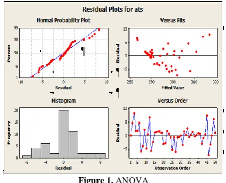
Three assumptions including normality of residuals, constant variance of the residuals and independency of the residuals in ANOVA (analysis of variance) table are also investigated which are illustrated in Figure 1. In Table 2, assuming ARL and ATS₀ ₀370.4, K 3,

 

E ts 1,E n

 

s 5 ,m1 ,B 1,n1

 

1,3





2 6,7,10 ,

n  t₁



0.01,0.1,0.25,0.5



and 



0.1,0.5,1,2 ,



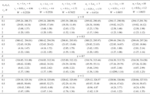
we have compared ARL and ATS₁ ₁ in terms of different measurement errors ratios;  



0,0.3,0.7,1



. From the results in Table 2, we can see that when there is no measurement errors (0), the out-of-controlARLs and

ATSs, are smaller, in comparisons to with measurement errors cases( 



0.3,0.7,1 )



. We can also see that, larger mean shift (), will result in smallerARL and ATS₁ ₁. These results are completely logical, because when there is measurement errors in the process, ARL and ₁

1

ATS are supposed to become worse and when we have a shift in the process mean, we wantARL and ₁ ATS₁ to be smaller, allowing the signal to occur sooner with bigger mean shifts.

Remember that smaller ARL and ₁ ATS₁ are always better. Based on Table 2, we can easily see that all of these conditions have been met for different combinations of the parameters 'values.

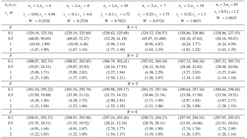
In Table 3, having all of the mentioned assumptions, except1 , we have compared ARL1 and ATS1 in terms of the number of each items' measurements;



1, 2,3, 4



m .

From the results of this table, we can easily see that when the number of measurements increases, the negative effect of measurement errors decreases (we will have smaller ARL1and ATS1), for different combinations of the parameters' values in the VSSI scheme.

In Table 4, we have performed sensitivity analysis for the parameter B. Note that since the parameter A has automatically been eliminated from our calculations (see the pervious section), its' value is irrelevant to our evaluations. As for parameter B, again with the same assumptions as the first analysis, except 1 and



1, 2,3, 4



B ,we can easily see in Table 4 that larger B will result in better performance in detecting a signal (we will have smaller ARL1 and ATS1).

Figure 1. ANOVA

TABLE 1. ANOVA which shows the effect of factors on the response variable

Source DF Seq SS Adj SS Adj MS F P

 1 873.52 532.93 532.93 49.51 0.00

m 1 299.60 5.89 5.89 0.55 0.462

B 1 1107.47 9.36 9.36 0.87 0.355



*m 1 131.49 133.52 133.52 12.40 0.001



*B 1 514.29 219.61 219.61 20.40 0.000

m*B 1 173.88 2.06 2.06 0.19 0.664

*m*B 1 52.85 52.85 52.85 4.91 0.030

Error 62 667.39 667.39 10.76

(6)

TABLE 2. (ARL ₁andATS₁) when ARL =ATS₀ ₀370.4,K 3,m1,B 1

1, ,1 1

n n t

2,W t

1 1, 2 6

n  n 

1 0.01, 2 4.96 t  t 

0.2526

W 

1 1, 2 6

n  n 

1 0.1, 2 4.6

t  t 

0.2526

W 

1 1, 2 10

n  n 

1 0.1, 2 1.72

t  t 

0.7622

W 

1 3, 2 7 n  n 

1 0.25, 2 1.75

t  t 

0.6724 W 

1 3, 2 10

n  n 

1 0.25, 2 1.3

t  t 

1.0633

W 

1 3, 2 10

n  n 

1 0.5,2 1.2

t  t 

1.0633

W 

𝛿 𝛾 = 0

0.1 (295.24, 288.37) (295.24, 288.99) (293.39, 288.16) (295.02, 290.45) (294.17, 290.58) (294.17,291.78)

0.5 (29.05, 16.34) (29.05, 17.49) (18.30, 11.49) (26.34, 18.06) (19.82, 14.27) (19.82, 16.12)

1 (3.68, 1.37) (3.68, 1.58) (2.63, 1.72) (3.23, 1.78) (2.58, 1.68) (2.58, 1.98)

2 (1.20, 1.03) (1.20, 1.05) (1.52, 1.16) (1.17, 1.04) (1.23, 1.06) (1.23, 1.12)

𝛿 𝛾 = 0.3

0.1 (300.42, 294.01) (300.42, 294.59) (298.81, 293.93) (300.23, 295.97) (299.49, 296.15) (299.49, 297.26)

0.5 (32.65, 19.20) (32.65, 20.42) (21.07, 13.68) (29.83, 21.03) (22.85, 16.87) (22.85, 18.86)

1 (4.16, 1.47) (4.16, 1.72) (2.85, 1.79) (3.62, 1.95) (2.81, 1.80) (2.81, 2.14)

2 (1.22, 1.04) (1.22, 1.05) (1.55, 1.18) (1.20, 1.05) (1.27, 1.08) (1.27, 1.14)

𝛿 𝛾 = 0.7

0.1 (316.85, 311.88) (316.85, 312.34) (315.89, 312.12) (316.74, 313.44) (316.30, 313.72) (316.30, 314.58)

0.5 (48.62, 32.80) (48.62, 34.24) (34.39, 24.94) (45.59, 35.11) (37.26, 29.79) (37.26, 32.28)

1 (6.63, 2.22) (6.63, 2.62) (4.00, 2.22) (5.66, 2.94) (4.07, 2.46) (4.07, 2.99)

2 (1.37, 1.06) (1.37, 1.09) (1.63, 1.26) (1.36, 1.10) (1.4290, 1.14) (1.43, 1.23)

𝛿 𝛾 = 1

0.1 (329.18, 325.34) (329.18, 325.69) (328.62, 325.69) (329.12, 326.57 (328.86, 326.86) (328.86, 327.53)

0.5 (68.05, 50.69) (68.05, 52.27) (52.29, 41.19) (65.07, 53.48 (56.16, 47.62) (56.16, 50.47)

1 (10.45, 3.89) (10.45, 4.48) (5.98, 3.14) (8.96, 4.87 (6.24, 3.77) (6.24, 4.59)

2 (1.67, 1.09) (1.67, 1.14) (1.76, 1.36) (1.62, 1.19 (1.61, 1.22) (1.61, 1.35)

TABLE 3. (ARL ₁andATS₁) when ARL =ATS₀ ₀370.4,K 3,1 ,B 1

1, ,1 1

n n t

2,W t

1 1, 2 6 n  n 

1 0.01, 2 4.96

t  t 

0.2526

W 

1 1, 2 6 n  n 

1 0.1, 2 4.6 t  t 

0.2526

W 

1 1, 2 10 n  n 

1 0.1, 2 1.72 t  t 

0.7622

W 

1 3, 2 7 n  n 

1 0.25, 2 1.75

t  t 

0.6724

W 

1 3, 2 10 n  n 

1 0.25, 2 1.3

t  t 

1.0633

W 

1 3, 2 10

n  n 

1 0.5,2 1.2

t  t 

1.0633

W 

𝛿 𝑚 = 1

0.1 (329.18, 325.34 (329.18, 325.69) (328.62, 325.69) (329.12, 326.57) (328.86, 326.86) (328.86, 327.53)

0.5 (68.05, 50.69 (68.05, 52.27) (52.29, 41.19) (65.07, 53.48) (56.16, 47.62) (56.16, 50.47)

1 (10.45, 3.89 (10.45, 4.48) (5.98, 3.14) (8.96, 4.87) (6.24, 3.77) (6.24, 4.59)

2 (1.67, 1.09 (1.67, 1.14) (1.76, 1.36) (1.62, 1.19) (1.61, 1.22) (1.61, 1.35)

𝛿 𝑚 = 2

0.1 (317.16, 312.23 (317.16, 312.67) (316.22, 312.46) (317.05, 313.77) (316.62, 314.05) (316.62, 314.91)

0.5 (49.02, 33.16 (49.02, 34.60) (34.74, 25.25) (45.98, 35.47) (37.63, 30.14) (37.63, 32.63)

1 (6.70, 2.24 (6.70, 2.65) (4.04, 2.24) (5.73, 2.97) (4.11, 2.48) (4.11, 3.02)

2 (1.38, 1.06 (1.38, 1.09) (1.64, 1.27) (1.37, 1.10) (1.43, 1.14) (1.43, 1.24)

𝛿 𝑚 = 3

0.1 (311.43, 305.98 (311.43, 306.47) (310.27, 306.13) (311.29, 307.67) (310.77, 307.93) (310.77, 308.87)

0.5 (42.41, 27.36 (42.41, 28.73) (29.02, 20.29) (39.42, 29.49) (31.49, 24.53) (31.49, 26.85)

1 (5.60, 1.87 (5.60, 2.21) (3.51, 2.03) (4.80, 2.50) (3.53, 2.17) (3.53, 2.62)

2 (1.31, 1.05 (1.31, 1.07) (1.60, 1.23) (1.30, 1.08) (1.37, 1.11) (1.37, 1.20)

𝛿 𝑚 = 4

0.1 (308.07, 302.33 (308.07, 302.85) (306.79, 302.41) (307.92, 304.10) (307.33, 304.33) (307.33, 305.33)

0.5 (39.07, 24.51 (39.07, 25.83) (26.25, 17.93) (36.12, 26.54) (28.48, 21.82) (28.48, 24.04)

1 (5.09, 1.71 (5.09, 2.02) (3.27, 1.94) (4.38, 2.29) (3.27, 2.03) (3.27, 2.44)

(7)

TABLE 4. (ARL ₁andATS₁) when ARL =ATS₀ ₀370.4,K 3, 1 ,m1

1, ,1 1

n n t

2,W t

1 1, 2 6 n  n 

1 0.01, 2 4.96

t  t 

0.2526

W 

1 1, 2 6 n  n 

1 0.1, 2 4.6 t  t 

0.2526

W 

1 1, 2 10 n  n 

1 0.1, 2 1.72 t  t 

0.7622

W 

1 3, 2 7 n  n 

1 0.25, 2 1.75

t  t 

0.6724

W 

1 3, 2 10 n  n 

1 0.25, 2 1.3

t  t 

1.0633

W 

1 3, 2 10

n  n 

1 0.5,2 1.2

t  t 

1.0633

W 

𝛿 𝐵 = 1

0.1 (329.19, 325.34) (329.19, 325.69) (328.62, 325.69) (329.12, 326.57) (328.86, 326.86) (328.86, 327.53)

0.5 (68.05, 50.69) (68.05, 52.27) (52.29, 41.19) (65.07, 53.480) (56.16, 47.62) (56.16, 50.47)

1 (10.45, 3.89) (10.45, 4.48) (5.98, 3.14) (8.96, 4.87) (6.24, 3.77) (6.24, 4.59)

2 (1.67, 1.09) (1.67, 1.14) (1.77, 1.36) (1.62, 1.19) (1.61, 1.22) (1.61, 1.35)

𝛿 𝐵 = 2

0.1 (308.07, 302.33) (308.07, 302.85) (306.79, 302.41) (307.92, 304.10) (307.33, 304.34) (307.33, 305.33)

0.5 (39.07, 24.51) (39.07, 25.83) (26.24, 17.93) (36.12, 26.54) (28.48, 21.82) (28.48, 24.04)

1 (5.09, 1.71) (5.09, 2.02) (3.27, 1.94) (4.38, 2.29) (3.27, 2.03) (3.27, 2.44)

2 (1.27, 1.05) (1.27, 1.07) (1.58, 1.21) (1.26, 1.07) (1.34, 1.10) (1.34, 1.18)

𝛿 𝐵 = 3

0.1 (301.54, 295.22) (301.54, 295.79) (299.98, 295.17) (301.35, 297.16) (300.64, 297.34) (300.64, 298.44)

0.5 (33.50, 19.88) (33.50, 21.12) (21.73, 14.22) (30.66, 21.74) (23.58, 17.50) (23.58, 19.52)

1 (4.28, 1.50) (4.28, 1.75) (2.90, 1.81) (3.71, 1.99) (2.87, 1.83) (2.87, 2.17)

2 (1.23, 1.04) (1.23, 1.06) (1.55, 1.18) (1.21, 1.06) (1.28, 1.08) (1.28, 1.15)

𝛿 𝐵 = 4

0.1 (298.91, 292.37) (298.91, 292.96) (297.24, 292.26) (298.72, 294.37) (297.95, 294.53) (297.95, 295.67)

0.5 (31.55, 18.31) (31.55, 19.52) (20.21, 12.10) (28.76, 20.11) (21.91, 16.06) (21.91, 18.01)

1 (4.01, 1.44) (4.01, 1.67) (2.78, 1.77) (3.50, 1.90) (2.74, 1.76) (2.74, 2.09)

2 (1.22, 1.03) (1.22, 1.05) (1.54, 1.17) (1.19, 1.05) (1.26, 1.07) (1.26, 1.14)

We also investigate the effect of measurement errors on the standard deviation of time to signal shown as Jensen et al. [11]:





1





1 (2) 2

1 1 ( 1 1

SDTS  bT I Q  2D_t IQ t t )(ATS) , (30)

where T

b =(b b₁, ₂) is the vector of starting probabilities, I is the identity matrix of order 2, Q₁ is the 2 2 transition probability matrix, _tT _



_{t t}_{2 1},



_{is the vector of} sampling intervals,D_tis the 2 2 diagonal matrix with the diagonal elements of t and t(2)contains the squares of the elements of the t vector. The results for different shift sizes and for K=3, m=1, B=1, E t

 

s 1, E n

 

s 5 , n₁2, n₂10, t₁0.1 can be seen in Figure 2.

Since the value of parameter B is determined when the measurement system is set up, now we evaluate the value of parameter m, for different values of parameter B and  . The result for the case of  0.5, K=3,

 

s 1

E t ,E n

 

s 3,n12 n25and t10.1 are displayed in Figures 3 and 4.

As we can see, in all cases, multiple measurements is only effective up to m=4, and more than that, it has negligible effect on the chart’s performance. Also, in the cases of B=4 and B=5 (𝐵 ≥ 4), multiple measurements has no effect on the chart’s performance.

Figure 2. SDTS ₁vs

(8)

Figure 4. ATS .₁vs m 0.1

5. A REAL CASE

In order to show an application for our VSSI scheme, we use the data from Costa and Castagliola [23]. Consider a 125 gr yogurt cup filling process. The quality characteristic Y is the weight of each cup.

After a long time study (Phase I), we know that 0 124.9

  and ₀ 0.76. From another study, we have:

0.24

 _M . Therefore: 0

0.24 0.316 .76

 



 M  

o . In this

example, we assume that, t₁0.3 , hr E t

 

s 1 ,hr

 

s 3

E n  , n₁2 , n₂5, K=3, A=0, B=1 and m=2. Having these assumptions and by using Equations (28) and (29),we have:W=0.9638 and t₂1.35 hrs.

We would like to take twenty samples in total. For the first sample size and sampling interval we choose:

1 2

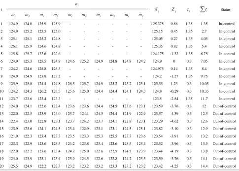
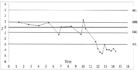
nn  andt  t₂ 1.35. Having calculated Z_i for each sample using Equation (10), for other sample sizes and sampling intervals we use the mentioned methodology in Section 3. You can see the final results in Table 5 and also graphically in Figure 5. As it is clear from the results, from sample 12 on, after twelve hours, the process mean will shift below LCL, meaning a signal of an out-of-control situation. Therefore, corrective actions are required.

TABLE 5.Twenty samples of size 2 or 5 withm2,t₁0.3,t₂1.35,k 3,W 0.9638, B=1,0.316and ₀ 124.9

i

i n

i X

i

Z t_i



ti Status

1

m m₂ m₁ m₂ m₁ m₂ m₁ m₂ m₁ m₂

1 124.9 124.8 125.9 125.9 - - - 125.375 0.86 1.35 1.35 In-control

2 124.9 125.2 125.5 125.0 - - - 125.15 0.45 1.35 2.7 In-control

3 125.1 125.1 125.2 124.8 - - - 125.05 0.27 1.35 4.05 In-control

4 126.1 125.9 124.6 124.8 - - - 125.35 0.82 1.35 5.4 In-control

5 125.8 125.7 122.6 122.6 - - - 124.175 -1.32 1.35 6.75 In-control

6 124.9 125.3 125.5 124.8 124.6 125.2 124.9 124.8 124.8 124.2 124.9 0 0.3 7.05 In-control

7 124.2 124.6 125.8 125.3 - - - 124.975 0.14 1.35 8.4 In-control

8 124.9 124.9 123.8 123.2 - - - 124.2 -1.27 1.35 9.75 In-control

9 125.9 125.8 124.4 124.8 126.3 125.7 124.9 125.2 125.2 125.1 125.33 1.23 0.3 10.05 In-control

10 124.2 124.3 126.2 125.5 125.6 125.0 124.4 124.4 124.1 124.3 124.8 -0.29 0.3 10.35 In-control

11 123.7 123.6 123.4 123.3 - - - 123.5 -2.54 1.35 11.7 In-control

12 124.0 124.1 122.6 122.4 123.6 123.6 124.4 124.5 123.6 123.1 123.59 -3.76 0.3 12 Out-of-control

13 122.0 122.5 123.9 124.0 123.7 124.1 124.3 124.4 121.9 122.9 123.37 -4.39 0.3 12.3 Out-of-control

14 122.4 123.0 122.8 123.1 123.7 124.2 123.7 124.1 122.8 123.1 123.29 -4.62 0.3 12.6 Out-of-control

15 123.9 123.6 124.1 124.5 123.4 122.9 123.1 123.1 124.5 125.1 123.82 -3.10 0.3 12.9 Out-of-control

16 121.9 122.3 123.4 123.3 123.5 123.3 125.3 125.5 123.3 123.6 123.54 -3.91 0.3 13.2 Out-of-control

17 123.3 122.9 123.6 123.5 124.2 123.8 123.4 123.6 123.5 123.4 123.52 -3.96 0.3 13.5 Out-of-control

18 122.0 122.2 123.6 123.4 124.7 125.0 122.6 122.5 124.5 123.9 123.44 -4.19 0.3 13.8 Out-of-control

19 124.0 123.9 123.1 123.4 123.9 124.5 122.6 122.8 124.2 123.5 123.59 -3.76 0.3 14.1 Out-of-control

(9)

Figure 5.Z Control Chart based on the VSSI scheme

6. CONCLUSION AND FUTURE RESEARCHES

In this paper, the measurement errors under single and multiple measurement cases have been considered in a VSSI X control chart. Using a Markov Chain approach, we obtained out-of-control ARLs and ATSs for this scheme.

First, we performed ANOVA to test the effect of  , m, B, and their interactions on the ATS and we found that each interaction involving is significant. Evaluating the effect of measurement errors on the VSSI X control chart, we concluded that higher measurement errors ratio () would result in larger out-of-control ATSs and ARLs, meaning worsened conditions. Later, we showed that, in order to decease the negative effect of measurement errors, one may consider multiple measurements of each item. The results also showed that increasing the value of constant B, decreases the negative effect of measurement errors as well. We also found out that the multiple measurements is effective up to 4 measurements, and also ifB4, then multiple measurements has no effect on the chart’s performance. Finally, we illustrated this scheme using a real case.

Investigating the effect of measurement errors on the performance of VSSI X control chart under the linearly increasing error variance can be considered as a future research.

Moreover, since our model is based on the assumption that the process parameters (₀ and )₀ are already known, future studies may include estimating them. Researchers may also consider the effect of measurement errors on the other univariate or multivariate adaptive control charts.

6. REFERENCES

1. Reynolds, M.R., Amin, R.W., Arnold, J.C. and Nachlas, J.A., "

X Charts with variable sampling intervals", Technometrics, Vol. 30, No. 2, (1988), 181-192.

2. Runger, G.C. and Pignatiello, J., "Adaptive sampling for process control", Journal of Quality Technology, Vol. 23, No. 2, (1991), 135-155.

3. Prabhu, S., Runger, G. and Keats, J., "X chart with adaptive sample sizes", The International Journal of Production Research, Vol. 31, No. 12, (1993), 2895-2909.

4. Costa, A.F., "X over-bar charts with variable sample-size",

Journal of Quality Technology, Vol.2, No.4, (1994), 155-163. 5. Zimmer, L.S., Montgomery, D.C. and Runger, G.C., "Evaluation

of a three-state adaptive sample size X control chart",

International Journal of Production Research, Vol. 36, No. 3, (1998), 733-743.

6. Costa, A.F., "X chart with variable sample size and sampling intervals", Journal of Quality Technology, Vol. 29, No. 2, (1997), 197-204.

7. Costa, A.F., "X charts with variable parameters", Journal of Quality Technology, Vol. 31, No. 4, (1999), 408-506. 8. Tagaras, G., "A survey of recent developments in the design of

adaptive control charts", Journal of Quality Technology, Vol. 30, No. 3, (1998), 212-220.

9. Zimmer, L.S., Montgomery, D.C. and Runger, G.C., "Guidelines for the application of adaptive control charting schemes",

10. Carot, V., Jabaloyes, J. and Carot, T., "Combined double

sampling and variable sampling interval X chart",

11. Jensen, W.A., Bryce, G.R. and Reynolds, M.R., "Design issues for adaptive control charts", Quality and reliability engineering international, Vol. 24, No. 4, (2008), 429-445.

12. Lim, S., Khoo, M.B., Teoh, W. and Xie, M., "Optimal designs of the variable sample size and sampling interval chart when process parameters are estimated", International Journal of Production Economics, Vol. 166, No., (2015), 20-35. 13. Prabhu, S.S., Montgomery, D.C. and Runger, G.C., "Combined

adaptive sample size and sampling interval X control scheme",

Journal of Quality Technology, Vol. 26, No. 3, (1994), 164-176.

14. Bennett, C.A., "Effect of measurement error on chemical process control", Industrial Quality Control, Vol. 10, No. 4, (1954), 17-20.

15. Kanazuka, T., "The effect of measurement error on the power of

X and R charts", Journal of Quality Technology, Vol. 18, No. 2, (1986), 91-95.

16. Linna, K.W. and Woodall, W.H., "Effect of measurement error on shewhart control charts", Journal of Quality Technology, Vol. 33, No. 2, (2001), 213.

17. Cocchi, D. and Scagliarini, M., "Effects of the two-component measurement error model", STATISTICA, Vol. 71, No. 3, (2011), 307-327.

18. Maleki, M., Amiri, A. and Ghashghaei, R., "Simultaneous monitoring of multivariate process mean and variability in the presence of measurement error with linearly increasing variance under additive covariate model", International Journal of Engineering-Transactions A: Basics, Vol. 29, No. 4, (2016), 471-480.

19. Hu, X., Castagliola, P., Sun, J. and Khoo, M.B., "The

(10)

measurement errors", Quality and Reliability Engineering International, Vol. 32, No. 3, (2016), 969-983.

20. Hu, X., Castagliola, P., Sun, J. and Khoo, M.B.C., "Effect of

measurement errors on the VSI X chart", European Journal of Industrial Engineering, Vol. 10, No. 2, (2016), 224-242. 21. Maleki, M.R., Amiri, A. and Castagliola, P., "Measurement

errors in statistical process monitoring: A literature review",

Computers & Industrial Engineering, Vol. 103, No., (2017), 316-329.

22. Montgomery, D.C. and Runger, G.C., "Gauge capability and designed experiments. Part i: Basic methods", Quality Engineering, Vol. 6, No. 1, (1993), 115-135.

23. Costa, A.F. and Castagliola, P., "Effect of measurement error and autocorrelation on the X chart", Journal of Applied Statistics, Vol. 38, No. 4, (2011), 661-673.