Volume 10, Number 1, pp. 1–11. http://www.scpe.org c 2009 SCPE
RECENT ADVANCES ON THE SIMULATION MODELS FOR AD HOC NETWORKS: REAL TRAFFIC AND MOBILITY MODELS
ARTA DOCI∗, LEONARD BAROLLI†, AND FATOS XHAFA‡
Abstract. In order to provide credible and valid simulation results it is important to built simulation models that accurately represent the environments were ad hoc networks will be deployed. Recent research results have shown that there is a disparity of 30% between protocol performance in real test beds and the one in simulation environments. In this paper we summarize the recent trends on the simulation models for ad hoc networks. First, we provide a survey of the synthetic and real traffic models used in ad hoc network simulation studies. Second, we select a representative of the most used mobility synthetic model, the real pedestrian mobility model, and the real vehicular model (for mixed traffic). We show that the real pedestrian and real vehicular model share common mobility characteristics: a) The transition matrix on both models illustrate that wireless nodes do not move from one location to another at random, but they are rather based on activities (work, shopping, college, gym); b) The dynamic membership property illustrates that nodes join and leave the simulation based on some variable distribution or patterns. Lastly, via simulations we show that when using realistic simulation models the simulation protocol performance closer reflects with the real test bed protocol performance.
Key words: wireless ad hoc networks, traffic model, mobility model, performance evaluations.
1. Introduction. Synthetic mobility models are mainly used to evaluate the protocol performance in wireless networks. The synthetic mobility models [1] are very useful, since they are easy to implement and mathematically tractable. However, the study at Uppsala University [2] shows that the wireless protocol per-formance in real test beds drops by 30% from the ones in the simulation platforms. The main reason for the disparity is the use of synthetic simulation models, including mobility and traffic models, which do not closely model the environments where the wireless networks will be deployed.
Recently, we have started to see a shift on using more realistic simulation models in the simulation evalua-tions. For example, the authors of [3] issue a ‘A call to arms: It’s time for REAL mobility models’, thus they design and implement a more realistic pedestrian mobility model. In addition, to further improve the validity and credibility of the simulation studies the authors of [4, 5] show that mobility and traffic are interconnected, as well as, implement a more realistic traffic model. The studies show that under more realistic mobility and traffic models the simulation protocol performance better reflects the protocol performance of real deployments. In addition, more realistic vehicular mobility models are implemented [6, 7, 8, 9, 10, 11, 12]. For example, the authors of [10] implement a more realistic vehicular model by using the publicly available TIGER (Topologically Integrated Geographic Encoding and Referencing) database from the U.S. Census Bureau, giving detailed street maps for the entire United States of America, and model the automobile traffic on these maps. First, the model can be very complex, since it needs to query the database for every location. Second, the database does not provide any speed limit information for each location. Lastly, the model makes assumptions about the speed distribution and other pertinent parameters. Specifically, the models do not take into account mixed traffic conditions [13, 14].
The focus of this paper is placed on the recent advances of the real traffic and mobility models for ad hoc networks. Specifically, the paper focuses on the more realistic simulation models, which are extracted from real user trace data on student campuses, GPS mounted devices on vehicles in city roads, and devices mounted on traffic lights for the mixed traffic conditions. For example, the paper highlights the similarities of real mobility models extracted from real user data for both the pedestrian and vehicular cases. In addition, it describes the realistic traffic models.
The contributions of this paper are three fold. First, it provides a survey of synthetic and real traffic models. Second, it shows that real mobility models for pedestrian and vehicular situations share common mobility characteristics. Third, it shows via simulations that real simulation models produce performance results that are closer to the real test beds evaluations, thus proposes that to improve the validity and the credibility of the ad hoc simulation results the use of real simulation models should be the preferred models.
∗Colorado School of Mines, Colorado, USA ([email protected]). Also, Head of Wireless Research at UNYT. †Fukuoka Institute of Technology, Fukuoka 811-0214, Japan ([email protected]).
‡Technical University of Catalonia, Barcelona, Spain ([email protected]).
2. Simulation Traffic Models. In this section we provide a survey of the synthetic simulation traffic models that are used in ad hoc network simulation studies. The most used synthetic traffic model is the Constant Bit Rate (CBR), which is described below. The main reason of the widespread use of the CBR is based on its simplicity on both design and implementation. In addition, we describe the implementation and design of a real traffic model. We show that the real traffic model suggests that traffic is not sent on constant streams, but rather on bursts.
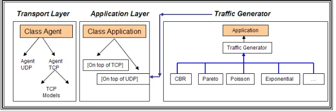
2.1. Synthetic Traffic Models. NS 2 views traffic as a two layer approach (as shown in Figure 2.1). The first layer implements transport protocols, Transmission Control Protocol (TCP) and User Datagram Protocol (UDP), while the second layer transmits application level data. For example, FTP and Telnet are two applications that generate traffic over TCP. On the other hand, Constant Bit Rate (CBR), Exponential, Pareto, and Poisson are applications that can be used to generate traffic over UDP.
Fig. 2.1.Traffic Generation Process in NS 2.
Traffic modelling can be classified under two main groups. The first group is that of applications that generate continuous traffic, namely the CBR that is the most used traffic model in ad hoc network simulation studies [15, 16]. In the second group, there are applications that model packet arrivals under Pareto, Exponential and Poisson Distribution [17, 18]. The latter, can be considered as applications that generate bursty traffic. We briefly describe these models next.
2.1.1. Constant Bit Rate Model. In this model source nodes generate traffic at a constant rate that are sent every interval ∆T seconds, which is defined by the user. For example, many sensor network applications generate constant bit rate traffic. In most ad hoc network applications wireless nodes do not send traffic continuously.
2.1.2. Exponential and Poisson Models. The exponential traffic model sends traffic during an ‘on’ state and does not send any traffic during the ‘idle’ state. The traffic is generated during the ‘on’ state with the following parameters: the packet size, the traffic rate, and the burst time1.
The exponential distribution can be viewed as a Poisson process when setting the variable burst time to zero and the variable traffic rate to a large value. In general, the packet inter-arrival times in the Poisson process are exponentially distributed. The probability distribution function is given by Eq. (2.1) and the density function is given by Eq. (2.2).
F(t) = 1−exp−λt, whereλis arrival rate (2.1)
f(t) =λexp−λt. (2.2)
2.1.3. Pareto Model. The Pareto traffic model also has the ’on’ and ’idle’ states, as the exponential traffic model. The packet arrival times of the Pareto distribution are independent and identically distributed, which means that each arrival time has the same probability distribution as the other arrival times and all are mutually independent. The two main parameters of the Pareto process are the shape and the scale parameter. The probability distribution function is given by Eq. (2.3) and the density function is given by Eq. (2.4).
F(t) = 1−
b
t
a
, wherea, b≥0 andt≥0 (2.3)
f(t) = ab a
ta+1 fort≥b, (2.4)
whereais the shape parameter andb is the scale parameter.
2.2. Real Traffic Model. Real traffic models have not been used much in the simulation evaluations. The main reason is the lack of the implementation, which are freely available to the research community. In this section we describe RealTrafficGen [5] model, which stands for real traffic generator. RealTrafficGen is interconnected with RealMobGen [3] mobility model and retrieves the dynamic membership of the wireless nodes, but it also adds three new features:
1. The generated traffic is dependent on the location, thus this model introduces distributions for each hotspot (based on real data).
2. Mobile nodes send more traffic then stationary wireless nodes, due to forwarded traffic from different hotspots, as well as their own traffic. This is the first model that differentiates the amount of traffic generated by the type of the node.
3. Traffic is likely to satisfy self-similarity property, rather then stationary distributions, due to diurnal circle; it is implemented as Weibull distribution.
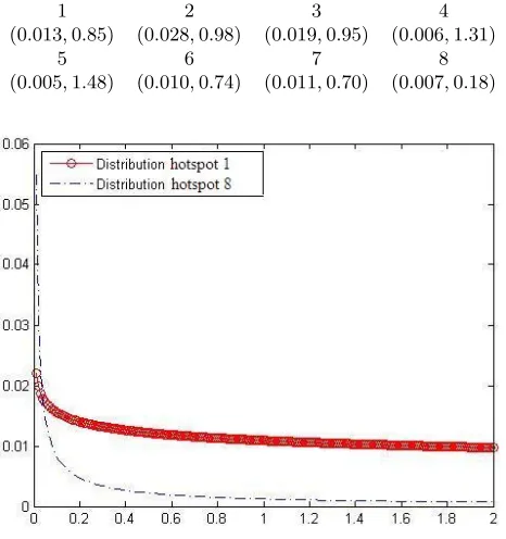
The model createsHotspotTrafficArray(see an example below). The first and third rows provides the hotspot number, while the second and forth rows shows the traffic flow on the respective hotspot, which is a Weibull distribution with parameters the shape (β) and mean (µ). For example, the Weibull distributions for hotspot 1 and hotspot 8 are shown in Figure 2.2.
1 2 3 4
(0.013,0.85) (0.028,0.98) (0.019,0.95) (0.006,1.31)
5 6 7 8
(0.005,1.48) (0.010,0.74) (0.011,0.70) (0.007,0.18)
Fig. 2.2.Weibull probability distribution function for hotspot 1 and 8.
3. Mobility Models. The main characteristics of a mobility model are speed, pause distribution, and direction of movement. In this section we describe one representative of the following simulation mobility models: synthetic, real pedestrian, and real vehicular (mixed traffic case).
node randomly picks up a destination independent of their initial positions and moves toward it with speed chosen uniformly on the interval (v0;v1). Nodes pause upon reaching each destination. The process is repeated until the allotted simulation time is reached.
The main advantage of RWM is its simplicity. On the other hand it has two major drawbacks. First, the direction of movement is not random. Second, the nodes do not start and remain in the simulation for the entire simulation time.
3.2. Real Pedestrian Mobility Model. In this section we describe RealMobGen, which is a hybrid model that is based on Dartmouth’s model of mobile network traces [22] and USC’s WWP [20] survey collected from the students on campus. The model closely mimics the environments where ad hoc networks will likely be deployed, since it borrows its characteristics from models derived from real user traces. Another feature of RealMobGen, that is not existent in any other current mobility model, is the classification of nodes as stationary (46% of the nodes) and mobile (54% of the nodes). The ratio of stationary vs. mobile nodes was borrowed from the Dartmouth model.
The stationary nodes select a location based on a transition matrix that defines the probabilities for moving from one point to another. Once a location is selected, a node is turned on for a time drawn from the exponential distribution of start time for the stationary nodes. Stationary node stays at the selected location until the allotted stationary end time. The mobile nodes, also, select a start location based on the transition matrix. The mobile node enters the simulation at a time drawn from the mobile node start time. The node pauses at the selected location until the allotted pause time from mobile pause time exponential distribution. After the pause time is up, the mobile node selects the next location based on the transition matrix and moves there not in a straight line but following data that supports movements along popular roads and turns. The mobile node repeats the pattern ’pause-select next location - move there’ until allotted mobile simulation end time.
RealMobGen shows that wireless nodes tend to cluster around popular locations, i. e., cafeteria, gym, classes, and library. We believe that RealMobGen is the first mobility model (we are not aware of any other models) that implements the dynamic characteristic of wireless devices in NS 2, devices join and leave the network at different times. RealMobGen addresses the drawbacks present in the RWM by implementing the following new features:
Feature 1: Wireless Nodes are clustered around popular hotspots. For example, Figure 3.1 shows a snapshot of RealMobGen with 150 nodes, which are clustered around 14 hotspots.
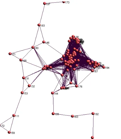
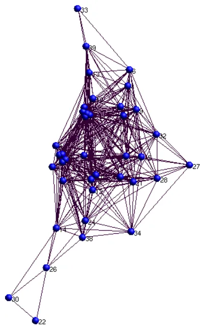
Feature 2: Wireless Nodes posses dynamic membership. For example, Figure 3.2 shows the dynamic mem-bership of 60 nodes.
Fig. 3.2.Dynamic Membership of 60 Nodes.
Feature 3: Nodes are classified on two flavors, namely stationary and mobile (stationary (46%)of the nodes and mobile (54% of the nodes). The ratio of stationary vs. mobile nodes was borrowed from the Dartmouth model.
Feature 4: Moving from one point to another is done via waypoints, instead of a straight line.
3.3. Real Vehicular Mobility Model. MixMobGen [26] is based upon the data collected by the Indian Institute of Technology [13] and from the Battelle Memorial Institute [14]. Both data sets have automatically collected mixed traffic data. MixMobGen is the first mobility model, we are not aware of any other one, that presents mixed traffic conditions by realistically implementing the speed as a bimodal distribution, the direction of movement based on a probability transition matrix, and the wireless nodes to poses the dynamic membership property (join and leave the simulation at some random time).
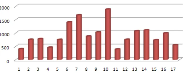
3.3.1. Data Sets. The first data set [13] was collected on 17 different data sections of the national and state highways in different parts of India, which were chosen to have a wide variation of fast vs. slow moving vehicles. The data collected on each section involved 2 hours of a typical weekday. (Refer to Figure 3.3 for a summary of the traffic sample size on each data section). For example, as shown in the Figure 3.3, the sample size on data section 6 is 1,407 vehicles.
Fig. 3.3.Number of the vehicles sampled on 17 data sections.
On each data section, different ratios of fast moving vehicles vs. slow moving vehicles were captured. The hypothesis of the study was:
Hypothesis: Speed Data distribution on mixed traffic conditions does not follow normal distribution.
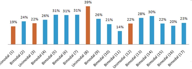
on the other 13 data sections. Furthermore, the graph shows that the bimodality of the data is not correlated to the volume of the fast vs. slow moving vehicles. For example, bimodality is supported when the ratio of slow moving vehicles was 14% on data section 11 or as high as 31% on data sections 5, 6, and 7. Analogously, the distribution was unimodal at low ratio of slow moving, i. e., 19% on data section 1 or at high ratio, i. e., 39% on data section 8.
Fig. 3.4.Ratio of the Slow Moving Vehicles and the Speed Distributions.
The second data set [14] covered the Lexington area of approximately 461 square miles with a total popu-lation of approximately 350,000. The sample was comprised of 100 households and included data collected via GPS mounted systems in the cars, which provides useful information for the mobility parameters that could not be extracted from the first data set, including direction of movement, trip start times, and dynamic membership properties.
The second data set reveals that the direction of movement is not random, but rather it is based on person’s activities. For example, on the case of traveling on local streets the purpose of trips was classified as follow:
Work Place 10%
Social/Recreational Activity 13.8%
Eat Out 15.8%
Shopping 14.9%
In addition, it emphasizes that nodes posses dynamic membership, thus are not in the simulation during the entire simulation time, but rather a fraction of the simulation time.
3.3.2. MixMobGen Parameters. In this section we discuss the parameters of the MixMobGen and the implementation choices in NS 2.
Speed Distribution. Speed distribution is extracted from the first data set [13], which shows that on the 13 out of the 17 of the data sections the speed of mixed traffic is best modeled by bimodal distribution. For example, on the Table 3.1 we show 13 data points collected at data section 6.
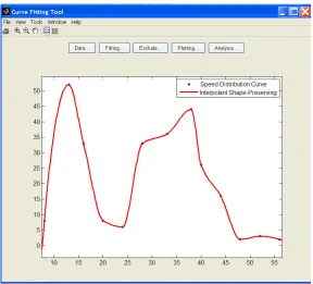
We assessed many distributions to graph the data, however we adopted the interpolation [27] method, which is the process of defining a function that takes on specified values at specified points (As shown in Figure 3.5). The figure and the study supports that the speed distribution is bimodal with the mean to be12.5 on the first peak and the mean to be37.5 on the second peak.
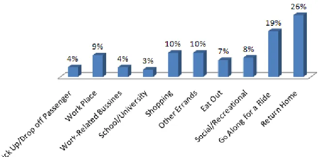
Direction of Movement. Wireless devices are carried by humans, thus the human movements would be the best approximation to the mobility patterns of the mobile nodes. We are aware that humans do not move at random, but rather based on activities. The data collected on Lexington area supports that humans move based on activities and the findings are summarized in Figure 3.6. We implemented this feature by introducing a T ransitional Destination P rob M atrix, which places a weight of 0.1 on the Shopping and Other Errands activities, or a weight of 0.26 on the Return Home activity.
Table 3.1 Speed Distribution Data
Speed (kmph) Probability Density
8 8
13 52
16 33
20 8
24 6
28 33
33 36
38 44
40 26
44 18
48 2
52 3
56 2
Fig. 3.5.Shape-preserving interpolation curve on the data collected in data section6.
In the implementation phase we introduced the array Start time of T rip, which has the percentage of the nodes that become active at time 0 (of the simulation). For example, 27% of the nodes become active at time 0), 5, 10, and (increments of 5 until the full hour is reached). In addition, we introduce the array the Active time of N odes, which presents the weights of the trip lengths.
Fig. 3.6. Destinations (As%of trips).
Fig. 3.7.Length of Trips.
Algorithm 1:M ixM obGen.
Input: Simulation Time (T); Number of Nodes (N);
1: ComputeT ransitional Destination P rob M atrix
2: ComputeStart time of T ripas a function of N
3: ComputeActive time of N odes as a function of N, T
4: INITIALIZATION 5: foreach nodeǫNdo
6: InitialLocation from theT ransitional Destination P rob M atrix
7: Speed (S) from the BimodalSpeed Distribution
8: ActiveTime from theActive time of N odes
9: TripStartTime fromStart time of T rip
10: end for
11: foreach nodeǫNdo
12: Select Destination (D) to move to from theT ransitional Destination P rob M atrix
13: Move toward D with speed S from Initial Location
14: if upon reaching D the node is still ACTIVEthen 15: Select new Destination and Speed
16: Move toward the new destination with the new speed
17: end if 18: end for
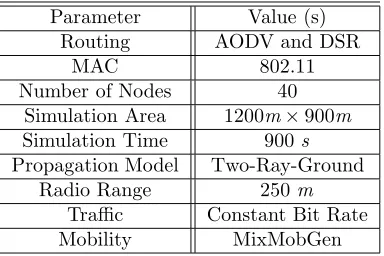
4. Protocol Performance Evaluations. The MixMobGen mobility was used to generate the movement pattern of the wireless nodes. mobility. In the routing layer AODV [24] and DSR [21] were selected, since they are the most used ones in the performance evaluations studies. The propagation model is the two-ray-ground [25]. The parameters that were not varied in the simulations were the number of nodes set to 40, simulation area 900m×1200m, simulation time set to 900s, the IEEE 802.11 [28] as the protocol for the medium access control (MAC) layer model.
We summarize in Table 4.1 the parameters used in the simulation.
Table 4.1 Simulation Parameters.
Parameter Value (s)
Routing AODV and DSR
MAC 802.11
Number of Nodes 40
Simulation Area 1200m×900m
Simulation Time 900s
Propagation Model Two-Ray-Ground
Radio Range 250m
Traffic Constant Bit Rate
Mobility MixMobGen
In addition, the derived parameters that are calculated from the number of nodes (40); the simulation area (900m×1200m); and the transmission range (R=250m) are provided below (for further explanations on each of the derived parameters we refer the reader to [29].)
Node Density: Number of nodes divided by the simulation area. In our case it is (900×1200)/40, thus 1 node for 27,000m2.
Coverage Area: Area with the transmission range as radius. In our case it is Π∗R2=196,349m2.
Maximum Path Length: The diameter of the rectangle 900m×1200mequals to 1500.
The network Diameter: The maximum path length divided by the transmission range, which in our case turns out to be 6Hops.
Network connectivity no edge effect: The coverage area by the node density, which turns out to be 7.27
Hops.
The performance metric used in this simulation evaluations isAvailability, which is a performance metric that takes into account the dynamic membership and we define it hereby.
Availability: We define Availability as the ratio between the number of packets sent by the source and the number of packets received by the destination, while the node is active.
MixMobGen shows that nodes are clustered around the main activities and their probabilities are defined by theT ransitional Destination P rob M atrix. For example, Figure 4.1 shows the visualization of MixMobGen on 40 nodes.
The traffic file is generated with three different sources (10,20,30) sources, respectively, 40 nodes, and the rate of generating packets was set to 4 packets. Each data point represents an average offifty runs with different traffic and different randomly generated mobility scenarios. The results of the experiments are summarized in Table 4.2. The results, also, include the 95% confidence intervals (CI) for validation of the experiments.
Table 4.2
Performance evaluation under MixMobGen.
Number of Availability: 95% CI: AODV Availability: 95% CI: DSR Sources AODV 95% CI: AODV DSR 95% CI: DSR 30 55.65% 55.65±4.03 56.11% 56.11±4.16
20 66.64% 66.64±4.22 66.48% 66.48±4.68
Fig. 4.1. MixMobGen on 40 Nodes.
5. Conclusions. In this paper we first described the synthetic mobility and traffic models. Specifically, we described in detail three real simulation models, namely: RealTrafficGen, RealMobGen, and MixMobGen. We believe that the mobility generator should adjust automatically to pedestrian mobility patterns, fast moving traffic, and mixed traffic. Therefore, in the future plan to design Knob Mobility Generator, which is based on the context can automatically adjust to the proper mobility model.
Furthermore, MixMobGen and RealMobGen suggest that mobility models that are extracted from real user data posses mobility characteristics that are rather different from the synthetic mobility models. When we evaluate the protocol performance using realistic mobility models, the performance drops significantly from the evaluations done when using synthetic mobility models.
The realistic mobility models shed new light into the ad hoc protocol design, as well. For example, the realistic mobility models show that nodes tend to cluster around popular locations. When the nodes are within the cluster they tend to be less mobile, but when they are between the clusters the nodes tend to be more mobile. However, none of the popular protocols captures this reality. In the future, we are going to address ad hoc protocol design based from on the real data sets collected for real world scenarios.
Lastly, we believe that realistic simulation models significantly improve the credibility and validity of the simulation models. This paper shows that when using more realistic simulation models, the protocol performance more closely reflects the one in the real test beds. In addition, the paper points out that there are similarities between pedestrian mobility models and mixed traffic condition mobility models. The main similarities are:
• Direction of movement: It is based on people activities.
• Dynamic Membership: Wireless Nodes join and leave the network dynamically.
• Transition Matrix : Moving from one location to another is based on weighted probabilities.
REFERENCES
[1] T. Camp, J. Boleng, and V. Davies,A survey of mobility models for ad hoc network research, Wireless Communications and Mobile Computing, vol. 2, no. 5, pp. 483–502, 2002.
[2] E. Nordstr¨om, P. Gunningberg, C. Rohner, and O. Wibling,Evaluating wireless multi-hop networks using a combination of simulation, emulation, and real world experiments. InMobiEval’07: Proceedings of the 1st International Workshop on System Evaluation for Mobile Platforms, pages 29–34, 2007.
[3] C. Walsh, A. Doci, and T. Camp,A call to arms: it’s time for real mobility models, vol. 12, no. 1, pp. 34–36, 2008. [4] A. Doci, Interconnected traffic with real mobility tool for ad hoc networks,International Conference on Parallel Processing
Workshops, International Conference on, vol. 0, pp. 204–211, 2008.
[5] A. Doci and F. Xhafa,WIT: A Wireless Integrated Traffic Model Mobile Information Systems Journal (4), pp 1–17, IOS Press, 2008.
[6] F. K. Karnadi, Z. H. Mo, and K.C. Lan,Rapid generation of realistic mobility models for Vanet, pp. 25062511, 2007. [7] D. R. Choffnes and F. E. Bustamante,An integrated mobility and traffic model for vehicular wireless networks, in VANET
’05: Proceedings of the 2nd ACM international workshop on Vehicular ad hoc networks, pp. 69–78, 2005.
[8] R. Mangharam, D. S. Weller, D. D. Stancil, R. Rajkumar, and J. S. Parikh,Groovesim: a topographyaccurate simulator for geographic routing in vehicular networks, Proceedings of the 2nd ACM international workshop on Vehicular ad hoc networks, pp. 5968, 2005.
[9] A. Jardosh, E. M. Belding-Royer, K. C. Almeroth, and S. Suri,Towards realistic mobility models for mobile ad hoc networks, Proceedings of the 9th annual international conference on Mobile computing and networking, pp. 217–229, 2003. [10] A. K. Saha and D. B. Johnson,Modeling mobility for vehicular ad-hoc networks, Proceedings of the 1st ACM international
workshop on Vehicular ad hoc networks, pp. 91–92, 2004.
[11] N. Potnis and A. Mahajan, Mobility models for vehicular ad hoc network simulations, Proceedings of the 44th annual Southeast regional conference, pp. 746–747, 2006.
[12] R. Baumann, S. Heimlicher, and M. May, Towards realistic mobility models for vehicular ad-hoc networks, In Mobile Networking for Vehicular Environments, pp. 73–78, 2007.
[13] P. Dey, S. Chandra, and S. Gangopadhaya,Speed distribution curves under mixed traffic conditions, Journal of trans-portation engineering, vol. 132, no. 6, pp. 475–481, 2006.
[14] Lexington area travel data collection test, final report: Global positioning systems for personal travel surveys, Battelle Memorial Institute, URL:http://www.fhwa.dot.gov/ohim/lextrav.pdf, 1997.
[15] J. Broch, D. A. Maltz, D. B. Johnson, Y.C. Hu, and J. Jetcheva, A performance comparison of multi-hop wireless ad hoc network routing protocols. InMobiCom’98: Proceedings of the 4th annual ACM/IEEE international conference on Mobile computing and networking, pages 85-97. ACM Press, 1998.
[16] S. R. Das, C. E. Perkins, and E. E. Royer, Performance comparison of two on-demand routing protocols for ad hoc networks. InINFOCOM (1), pages 3–12, 2000.
[17] T. Karagiannis, M. Molle, M. Faloutsos, and A. Broido, A nonstationary poisson view of internet traffic. In INFO-COM 2004: Proceedings of twenty-third AnnualJoint Conference of the IEEE Computer and Communications Societies, volume 3, pages 1558 - 1569, 2004.
[18] L. Kleinrock, Queueing Systems, Vol. II Computer Applications. Wiley, New York, USA, 1976.
[19] T. V. Group, The network simulator—NS 2. URL:http://www.isi.edu/nsnam/ns/Page accessed as of May 30th, 2006. [20] W. J. Hsu, K. Merchant, H. W. Shu, C. H. Hsu, and A. Helmy, Weighted waypoint mobility model and its impact on ad
hoc networks. SIGMOBILE Mobile Computer Communications Review, 9(1): 59–63, 2005.
[21] D. Johnson and D. A. Maltz, Dynamic source routing in ad hoc wireless networks. InMobile Computing, volume 353. Kluwer Academic Publishers, 1996.
[22] M. Kim, D. Kotz, and S. Kim, Extracting a mobility model from real user traces. InINFORCOM: Proceedings of the 25th Annual Joint Conference of the IEEE Computer and Communications Societies, pages 1–13, 2006.
[23] X. G. Meng, S. H. Y. Wong, Y. Yuan, and S. Lu, Characterizing flows in large wireless data networks. In MobiCom’04: Proceedings of the 10th annual international conference on Mobile computing and networking, pages 174–186, New York, NY, USA, 2004. ACM.
[24] C. Perkins and E. Royer,Ad-hoc on-demand distance vector routing. InProceedings of the 2nd IEEE Workshop on Mobile Computing Systems and Applications, pages 90–100, 1999.
[25] T. Rappaport,Wireless Communications: Principles and Practice. Prentice Hall PTR, Upper Saddle River, NJ, USA, 2001. [26] A. Doci, L. Barolli, and F. Xhafa,MixMobGen—a realistic Mixed traffic Mobility Generator for ad hoc network simulations
CISIS: Wireless and Mobile Networking, 2009.
[27] D. Kahaner, C. Moler, and S. Nash, Numerical methods and software. Upper Saddle River, NJ, USA: Prentice-Hall, Inc., 1989.
[28] Wireless lan medium access control (mac) and physical layer (phy)specifications. Technical report, IEEE Computer Society LAN MAN Standards Committee, 1997.
[29] J. Boleng, W. Navidi, and T. Camp, Metrics to enable adaptive protocols for mobile ad hoc networks. InInternational Conference onWireless Networks, pages 293–298, 2002.
Edited by: Fatos Xhafa, Leonard Barolli
Received: September 30, 2008