Scalable Computing: Practice and Experience
Volume 19, Number 3, pp. 223–244. http://www.scpe.org
ISSN 1895-1767 c
⃝2018 SCPE
EXACT AND HEURISTIC DATA WORKFLOW PLACEMENT ALGORITHMS FOR BIG DATA COMPUTING IN CLOUD DATACENTERS
SONIA IKKEN∗, ERIC RENAULT†, ABDELKAMEL TARI‡, AND M. TAHAR KECHADI§
Abstract. Several big data-driven applications are currently carried out in collaboration using distributed infrastructure. These data-driven applications usually deal with experiments at massive scale. Data generated by such experiments are huge and stored at multiple geographic locations for reuse. Workflow systems, composed of jobs using collaborative task-based models, present new dependency and data exchange needs. This gives rise to new issues when selecting distributed data and storage resources so that the execution of applications is on time, and resource usage-cost-efficient. In this paper, we present an efficient data placement approach to improve the performance of workflow processing in distributed datacenters. The proposed approach involves two types of data: splittable and unsplittable intermediate data. Moreover, we place intermediate data by considering not only their source location but also their dependencies. The main objective is to minimise the total storage cost, including the effort for transferring, storing, and moving that data according to the applications needs. We first propose an exact algorithm which takes into account the intra-job dependencies, and we show that the optimal fractional intermediate data placement problem is NP-hard. To solve the problem of unsplittable intermediate data placement, we propose a greedy heuristic algorithm based on a network flow optimization framework. The experimental results show that the performance of our approach is very promising.
Key words: Big data placement, Data workflow management, Dataflow model, Distributed datacenters, Storage cost mini-mization, Scalable storage and computing
AMS subject classifications. 15A15, 15A09, 15A23
1. Introduction. This study addresses the problem of intermediate data placement in big data-driven ap-plications. These data are usually stored in multiple cloud datacentres. The main goal is to be able to efficiently process and share them between a set of tasks (jobs or services) according to their needs, dependencies, and their resource requirements. In other words, the problem is how to efficiently store and access the intermediate data taking into account the inter- and intra-job (process) dependencies. These jobs can be any traditional process at the level of the operating system or services at the application level. Because of the popularity of the service delivery model, the cloud consists of a set of services that should be provided to the clients. At a very large scale (cloud scale), a huge number of activities coexist generating or consuming huge amount of intermediate data, which are stored in the form of files, called temporary files, in datacentres. From the point of view of data usage, this follows a workflow depending on the dynamic nature the execution of these services. These dependencies are of very high importance for the correct execution of the services that were provided to the clients. Each workflow has different requirements not only in the dependencies of its intermediate data files but also their sizes and types. Moreover, these services (jobs or set of tasks) can be initiated remotely from different geographic locations, which adds a level of complexity of how these data can be accessed without putting a significant stress on the cloud resources (bottlenecks, long waiting queues, etc.). Therefore, the way that these intermediate data files should be manipulated and managed must take into account their near future usage (frequency of use, life cycle, etc.). Accordingly, their management (storage, movement, processing, etc.) should be derived from the workflow of the jobs and services that are using them, which is called ”Data Workflow”.
This paper proposes a new approach that takes into account the types of dependencies and accesses to the intermediate data, as these are the key factors for improving big data-driven applications while leveraging cloud resources among the clients in an efficient and scalable manner. We start by formulating the intermediate data placement dependencies derived from multiple workflows running on distributed cloud datacenters. Then we model the whole system as a constrained optimization problem, where constraints represent the dependencies derived from the running workflows. The derived constrained optimization problem that includes storage cost is very complex. Two types of data are considered; the intermediate data that are used by the same job with
∗Faculty of Exact Sciences, University of Bejaia, 06000 Bejaia, Algeria, and Telecom SudParis, Samovar-UMR 5157 CNRS,
University of Paris-Saclay, France ([email protected], [email protected]).
†Telecom SudParis, Samovar-UMR 5157 CNRS, University of Paris-Saclay, France ([email protected]). ‡Faculty of Exact Sciences, University of Bejaia, 06000 Bejaia, Algeria ([email protected]).
their intra-dependencies from multiple tasks and intermediate data that are used by different jobs with their inter-job dependencies. Since intra-job dependencies can be split partially and placed on different locations (as in MapReduce), the problem is called minimum cost multiple-sources multicommodity flow problem (MCMF). Intermediate data dependencies that are used by different tasks (of a single job) can be split and kept in the same datacenter and preferably at the location of the task. We formulate the problem with these data as splittable demands which can be solved with an exact algorithm to obtain an optimal fractional solution. However, as most of these problems are NP-hard, it is difficult to obtain an optimal solution using exact methods for the variant that deals with unsplittable intermediate data from inter-job dependencies. Greedy approaches implement simple algorithms but effective for unsplittable flow problem [1, 2, 3, 4, 5], and they scale linearly with the number of instances. Their resolution techniques are adaptable to our intermediate data placement problem that the present paper deals with. Experimental results show that the proposed techniques are very promising for storage cost minimisation.
The rest of the paper is organized as follows: Section 2 summaries the related work. Section 3 introduces the system model and problem definition according to the cloud computing environment and data models. The proposed techniques for the optimal intermediate data dependencies placement are presented in Section 4. Section 5 discusses the performance evaluation and the simulation results. We conclude and give some future directions in Section 6.
2. Related works. We have thoroughly investigated recent research works on cloud ressource scheduling in the literature [31, 32, 33]. These works focus primarily on resource sharing and provisioning problems in order to either save energy consumption or reduce its costs by providing efficient application processing. Authors in [31], addressed the power consumption problem and network performance degradation by relying on an optimization model that is based on sliding-scheduled tenant request. The latter allows to manage application execution time as well as their resources for efficient placement and routing. Authors in [32], proposed a genetic algorithmic based heuristic methods to schedule tasks across limited resources, but restricted to use one global cost and time for multiple tasks execution. More recently, authors in [33], addressed the problem of resource scheduling of scientific workflow applications in cloud. They focus on reducing the cost of the communications and the information exchange time across a management framework of multiple-site awareness data administration. Nevertheless, these works did not address the problem of data workflow placement and the dependencies between resources.
Workflow scheduling problems [35, 36] in cloud environments are considered to be very challenging. Many strategies based-heuristic were proposed to solve the tasks scheduling problem without considering the data that are generated by these tasks. Authors in [35], proposed a meta-heuristic approach, called Hybrid GA-PSO (Genetic Algorithm-Particle Swarm Optimization), to solve the workflow tasks scheduling problem. The Hybrid GA-PSO algorithm returns a balanced solution for tasks distribution among different virtual machines in a cloud environment by considering both the total monetary cost and the execution makespan. While the PSO-based algorithm converges quickly to a local optimal solution, this can be far from the global optimal solution. In the same context, authors in [36] proposed a metaheuristic-based algorithm, called Hybrid Bio-inspired Metaheuristic for Multi-objective Optimization (HBMMO), to solve the multiple conflicting objectives optimization problem. The authors considered in their optimization some important requirements of the users or the providers, such as makespan, cost, and load balancing among virtual machines. The proposed HBMMO method optimizes the scheduling of tasks workflow in the cloud environment by considering a non-dominant sorting strategy which is a hybridization of the list-based heuristic algorithm PEFT (Predict Earliest Finish Time) [37] and the discrete version of the metaheuristic algorithm SOS (Symbiotic Organisms Search) [38].
com-munication and correlation is not considered. Authors in [6], proposed a strategy placement for large-volume user’s data while minimizing their operational costs of accommodating various social networks. The relation between the user community and dynamic maintenance of the placed user data in an evolving social network are considered, but the use of the data dependency aspects is not explored. In [7], the big data placement problem from a collaborative-aware environment that continuously generates data from different geographical locations has been studied. The authors developed a solution to save the high cost incurring when managing the distributed big data, and they proposed an approximation algorithm by reducing the data placement problem to the minimum cost multicommodity flow problem. Their solution addressed a data placement respecting a fair usage of the cloud services like the quality of service (QoS) requirement of cloud provider while savings computation and bandwidth costs. The solution is closely similar to our context but differs mainly on the con-ditions and characteristics of data workflow aspects and by no means disclosing intermediate data dependencies. They focused more on maximizing the system throughput in terms of data volume to be placed while saving the computing/storage and communication costs in the distributed datacenters. Sharing intermediate data from computation produced between different workflow MapReduce jobs is studied in [8]. The authors presented a scheduling technique for data-driven jobs sharing opportunities that involves the scan of the input file with the goal of maximizing the likelihood of sharing scans. A similar optimization approach is presented in [9]. A cost model is presented saving processing time and money for MapReduce jobs in order to define an optimization problem that finds an optimal grouping of set of queries and solves it using a dynamic programming approach. These works present a data-driven job scheduling issue which is not exactly the same as the data placement problem. These do not focus on the intermediate data scheduling optimization as well as the incurred storage cost.
Workflow scheduling problems [35, 36] in cloud environments are considered to be very challenging. Many strategies based-heuristic were proposed to solve the tasks scheduling problem without considering the data that are generated by these tasks. Authors in [35], proposed a meta-heuristic approach, called Hybrid GA-PSO (Genetic Algorithm-Particle Swarm Optimization), to solve the workflow tasks scheduling problem. The Hybrid GA-PSO algorithm returns a balanced solution for tasks distribution among different virtual machines in a cloud environment by considering both the total monetary cost and the execution makespan. While the PSO-based algorithm converges quickly to a local optimal solution, this can be far from the global optimal solution. In the same context, authors in [36] proposed a metaheuristic-based algorithm, called Hybrid Bio-inspired Metaheuristic for Multi-objective Optimization (HBMMO), to solve the multiple conflicting objectives optimization problem. The authors considered in their optimization some important requirements of the users or the providers, such as makespan, cost, and load balancing among virtual machines. The proposed HBMMO method optimizes the scheduling of tasks workflow in the cloud environment by considering a non-dominant sorting strategy which is a hybridization of the list-based heuristic algorithm PEFT (Predict Earliest Finish Time) [37] and the discrete version of the metaheuristic algorithm SOS (Symbiotic Organisms Search) [38].
The research works that considered data workflow features are presented in [10, 11, 12, 13, 14]. Nevertheless, the dynamic variation of inter and intra-jobs dependencies from the generated intermediate data was not addressed with the same focus. In [10], an adaptive data-task placement approach is proposed that reflects asynchronous coupling among tasks in order to reduce execution time and data movement overhead. The authors in [11] have dealt with improving the data workflow’s execution by clustering the interdependent datasets and distribute them intelligently onto the same datacenters to reduce data transfers. In [14], the authors established a data placement algorithm based on data dependency clustering and recursive partitioning. The aims of the algorithm are to reduce the amount of transmitted data and the time consumption during data-intensive application execution. The pursued strategy is extended with a heuristic to make frequent data movements occuring on high-bandwidth channels of the entire cloud system.
3. System model.
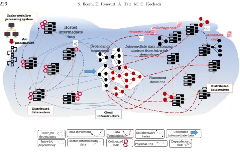
3.1. Cloud storage infrastructure and assumptions. For the intra- and inter-job data workflow place-ment problem depicted in Fig. 3.1, the objective is to route and store a set of intermediate data considering their dependencies generated by a collaborative tasks1 from multiple physical sites while saving their
opera-1
Fig. 3.1.The system architecture.
tional costs. Without loss of generality, we assume that the collaborative tasks, which process and generate new intermediate data files, are previously assigned to the cloud infrastructure (model task assignment offered by a cloud infrastructure). Since the intermediate data dependency placements are our most significant concern, we assume that the tasks were assigned to computing nodes following some simple model. The problem of placing the intermediate data files is close to the well-known MCMF problem; an optimization problem described in [15] that involves simultaneously shipping multiple commodities through a single graph, so the total flow obeys the arc capacity constraints by optimizing the cost.
The modeling starts by considering a set of geographically distributed datacenters2 as a directed
graph-based model G = (DC ∪A, E). It forms a cloud infrastructure and constructs a shared computation and storage limited to a set of resources for processing and storing the data workflow. Users, such as enterprises, institutions or researchers, that own and share a cloud infrastructure issued from providers, have an access to the distributed datacenters (DC) to process multiple collaborative tasks into multiple processing phases. The distributed datacenters known as storage containers cohabit with collaborative task Athrough one or multiple jobs r running in parallel [16]. A set of tasks are collocated on multiple source datacenters, and each task ar
i ∈Afrom job ris assigned to source datacenterdci. Let{ei,j, ej,j′} ∈E be the intermediate data transfer
and movement (initial and dynamic intermediate data routing respectively) links between source datacenterdci and destination datacenterdcjand between destination datacentersdcjand another destination datacenterdcj′,
which are geographically interconnected via the Internet. The placement of the intermediate data dependencies to the set of datacenter destinationsdcj∈DC is considered at the beginning of each phase.
3.2. Intermediate data dependency model. Placing intermediate data with the same correlation to a single destination datacenter can significantly decrease the amount of data dependency movements [17]. This leads to consider a vector of all intermediate data files denoted by ΦM and |ΦM| its size, representing the
2
correlations among them that are generated during the workflow phases divided into equal period of time t. These correlations, which reflect the intra- and inter-job dependencies from a set of intermediate data files, are recovered into dependency componentm∈M. M contains all the different components of dependency that are modeled by a Directed Acyclic Graph (DAG) which takes the advantage of a topology ordering, thus defining relations among nodes [18, 19]. The DAG represents a set of intermediate data files ϕm
ar
i(t). Let |ϕ
m ar
i(t)| be
their respective sizes. These data files have unavoidable complex dependencies that are generated by single task ar
i ∈A from jobr at source datacenter dci. In DAG, set of filesϕmar
i(t), from the inter-job dependencies,
are atomic and must be synchronized for their processing. By contrast, for the intra-job dependencies, these files are deduced from a partial correlation with an asynchronous processing [10]. Let ϕm(t) andϕmi (t) be the intermediate data of a single dependency component mgenerated at multiple datacenters and the single home datacenterdcirespectively and,|ϕm(t)|and|ϕmi (t)|be their respective sizes. At the end of each workflow phase, generated intermediate data fileϕm
i (t)∈Φmmust be outsourced and placed through data transfer linkei,j∈E from datacenterdci todcj for persistent storing or future reuse [20, 21]. It is important to note that the set of dependency componentsM and the related type are a predetermined value given by scientific user that can be obtained through the data analysis clustering method [22]. We assume that the intermediate data dependencies clustering is given a priori and is beyond the scope of the present work.
3.3. Capacity and cost model. To come up with an intermediate data dependency placement from the collaborative task workflow execution in cloud datacenters, we take into consideration the fact that all datacenters and network resources are limited [23, 24]. Thus, let Sj be the storage capacity of datacenter destination dcj ∈ DC, and Wi,j, Wj,j′ be the bandwidth capacities of the data file transfer and movement
links ei,j, ej,j′ ∈ E respectively. In order to manage and transfer these files, a data bandwidth denoted wϕ
is assigned for one unit of intermediate data file. During a run-time phase, the available amount of storage capacity in datacenterdcj, when transferring an amount of intermediate data filesϕmi (t), is denoted bysavaili,j (t). Let wavaili,j (t), wj,javail′ (t) be the available capacities of a data transfer and movement of links ei,j, ej,j′ ∈E. In
addition, transferring and storing the intermediate data dependencies from source datacenterdciinto destination datacenterdcj are facing in both storage resource cost and scale. However, they usually consume high costs in a cloud infrastructure due to an inefficient utilization of the resources [25]. In practice, these resource demands are leading to operational cost specifically for data transfers and storage costs (measured per one unit in GB) that embrace the usage-based pricing policy [9]. Moreover, reused intermediate data dependencies that are not locally stored but remotely served on data demands are led to an additional cost, as movement cost, which is deducted from their migration among datacenter destinations [14]. In fact, these operational storage costs are related to the size of the intermediate data files that are transferred, stored and moved among distributed datacenters according to their correlation during each run-time phase. Moreover, each datacenter destination dcj∈DCis preserved to the geographical area where it is located [26], thus holding a storage cost notedcsj. The
proportion of intermediate data dependencies ϕm of a single dependency component generated from multiple source datacenters and placed separately into different locationsdcj anddcj′ are led to a potential dependency
movement cost. For clear differentiation from the transfer cost, we assume that the cost of intermediate data movement is proportional to the number of intermediate data dependency files transmitted between datacenter destinations. Therefore, the movement cost is defined as the amount of data moved among two or multiple destination datacenters. Hence, each link ei,j, ej,j′ ∈E entry faces data bandwidth costcwφ.
For the sake of easier reading, Table 3.1 summarizes the notations used in the present work.
Table 3.1
Symbols for the model
Notation Description
G The cloud infrastructure (provider)
DC A set of distributed datacenters in cloud infrastructureG
t The run-time window which represents the homogeneous discrete time slot from generated collaborative data-tasks workflow processing A The set of collaborative tasks in distributed datacenterDC E The set of links among distributed datacenterDC
i, j, j′ Indices used to designate distributed datacenters. i belongs to source datacenterdci, whilejandj′belong to different destination datacenters (dcj anddcj′)
ei,j Data transfer link between source datacenter dci and destination data-center dcj
r Workflow job in the system
ar
i The collocated task in source datacenterdci
dci A source datacenter temporarily storing generated intermediate data from collocated taskar
i of job r∈R
dcj A datacenter destination where the intermediate data files are to be placed
M The set of dependency components in the system including correlation among generated intermediate data
ϕm(t) The intermediate data files of a single dependency componentm gener-ated in multiple datacenters at time slott, and|ϕm(t)| its size
ϕm
i (t) The intermediate data files generated in datacenterdcifrom dependency component m∈M at time slott, and|ϕm
i (t)|its size ϕm
ar
i(t) The intermediate data files generated by taskai
r of dependency
compo-nentmat time slott, and|ϕm ar
i(t)| its size
ΦM All generated intermediate data files in the system, and |ΦM|its size Lϕ The vector list of intermediate data of all dependency components m∈
M, m= 1, ..., k
wϕ The data bandwidth assigned to one unit of intermediate data fileϕmar i(t)
Wi,j The data bandwidth capacity of movement link ei,j∈E wavail
i,j (t) The available amount of data transfer link ei,j∈E at time slott Wj,j′ A data bandwidth capacity of movement linkej,j′ ∈E
wj,javail′ (t) The available amount of data transfer link ej,j′ ∈E at time slott
savail
i,j (t) The available amount of storage space when transferring an amount of intermediate data files from source datacenter dci to destination data-center dcj at time slott.
Sj The data storage capacity of destination datacenterdcj∈DC xm
i,j(t) A decision variable reflecting the amount of intermediate data flow mov-ing from source datacenterdci of dependency componentmto destina-tion datacenterdcj∈DC at time slott.
xm
j,j′(t) A decision variable reflecting the amount of intermediate data
depen-dency componentmmoving between destination datacentersdcj, dcj′ ∈
DC at time slott
csj The storage cost of one unit of intermediate data in datacenter
destina-tiondcj ∈DC
cwφ The data bandwidth cost of one unit of intermediate data
f(ϕm ar
i) A dependency component flows in graphGp
4.1. Exact algorithm. This section presents an exact analytical algorithm for splittable variant of the intermediate data dependency placement problem from multiple datacenters in cloud infrastructure G. The exact algorithm is an LP model with the inclusion of valid conditions expressed in the form of constraints or inequalities. Through the constraints of the problem, the intermediate data placement in a directed graph G = (DC∪A, E) at time slot t is to route and place intermediate data dependencies ϕm(t) ∈ ΦM that are considered as continuous commodity flows of dependency component m from multiple source datacenters to one or multiple destination datacenters while saving their transfer, storage and movement costs. A number of decision variables and valid inequalities (as listed for convenience in Table 3.1) are thus defined as follows:
1) Decision variables: Letxm
i,j(t)∈Rbe the intermediate data of one dependency componentmstanding for the amount of intermediate data dependency flows transferring from source datacenter dci at time slot t to destination datacenter dcj at time slot t+ 1 on link ei,j ∈ G. In order to take into account the amount of intermediate data dependencies that are moved among different destination datacenters dcj, dcj′, we add
variablexm
j,j′(t)∈R.
2) Flow conservation constraint: One typical constraint or requirement is to ensure that at all time, every flow through directed graph G is physically possible. First, we enforce flow continuity by making sure that the sum of intermediate data dependency flows leaving from source datacenter dci at time slot t−1 is equal to ϕm
i (t) which is the sum of flows arriving from the same datacenterdci that are considering the same dependency componentmat time slott. Formally:
∑
j∈DC xm
i,j(t)− ∑
j∈DC xm
j,i(t−1) =ϕmi (t) ∀m, t, i. (4.1)
3) Capacity constraint of intermediate data flows: Each intermediate data dependency flow xm i,j(t) may have its own individual capacity constraint which represents a lower bound on dependency component commoditym through linkei,j. This ensures the atomicity of lower boundϕm
ar
i(t) onx
m
i,j(t) of which all these flows take a same linkei,j, hence:
0≤ϕmar
i(t)≤x
m
i,j(t) ∀i, j, ari, m, t. (4.2)
4) Capacity constraint of data transfer links: InG, each linkei,jmay have a capacity constraint like the data bandwidth routing constraint. Equation (4.3) ensures that the routing of aggregate intermediate data dependencies is limited by the available amount of data bandwidth allocated on linkei,j at time slott:
∑
m∈M
wϕ· |ϕmi (t)| ·xmi,j(t)≤wi,javail(t) ∀i, j, t. (4.3)
Additionally, linkei,j is bounded by the data bandwidth capacity at all system execution time, hence: ∑
m∈M ∑
t∈T
wϕ· |ϕmi (t)| ·xmi,j(t)≤Wi,j ∀i, j. (4.4)
5) Capacity constraint of data movement links: InG, each linkej,j′ may have a capacity constraint
like the data bandwidth routing constraint. Equation (4.5) ensures that moving intermediate data dependencies is limited by the available amount of data bandwidth allocated on linkej,j′ at time slott:
∑
m∈M ∑
ar
i∈A
wϕ· |ϕm(t)−ϕmar i(t)| ·x
m
j,j′(t)≤wj,javail′ (t) ∀j, j′, t. (4.5)
Additionally, the link ej,j′ is bounded by the data bandwidth capacity at all system execution time, hence:
∑
m∈M ∑
ar i∈A
∑
t∈T
wϕ· |ϕm(t)−ϕmar i(t)| ·x
m
6) Capacity constraint of dependency component: A uniqueness constraint is used to ensure that the routed intermediate data dependency flows do not exceed the dependency corresponding component capacity. Formally:
∑
i∈DC
xmi,j(t)≤ϕmi (t) ∀j, m, t. (4.7)
7) Storage capacity constraint: Each destination datacenter has a limited amount of storage space available to share across all the intermediate data placement demands. This allows to host only a limited amount of intermediate data dependencies from source datacenterdci to destination datacenterdcj. Formally:
∑
m∈M
|ϕmi (t)| ·xmi,j(t)≤savaili,j (t) ∀i, j, t. (4.8)
For any intermediate data placement demands, the data routing must not exceed the total storage capacity at all system execution time. Formally:
∑
m∈M ∑
t∈T
|ϕmi (t)| ·xi,jm(t)≤Sj ∀i, j. (4.9)
8) Balancing constraint: Since the collaborative tasks in the workflow processing generate the inter-mediate data dependencies in multiple phases, these latter may vary over time in the distributed datacenter environment. In other words, the flow sequence of generated intermediate data dependencies changes as com-modity changes. Thus, the flows among the distributed datacenters must be balanced. Hence, source and sink nodesssourceandssinkare respectively introduced in graphG. Source nodessourceis connected to every source datacenter dci, and sink node ssink is connected to every destination datacenter dcj. Source and sink nodes are also subject to a constraint that enforces all the intermediate data dependency flows starting on ssource to ending at ssink. Formally:
∑
i∈DC
xmssource,i= ∑
j∈DC
xmj,ssink ∀m∈M (4.10)
9) Data transfer cost: Equation (4.11) denotes the data transfer cost on link ei,j which intermediate data dependency flows are routed.
C(wi,j) = ∑
i∈DC ∑
j∈DC ∑
m∈M ∑
t∈T
|ϕmi (t)| ·xmi,j(t)·wϕ·cwφ (4.11)
10) Storage cost: Equation (4.12) denotes the storage cost of destination datacenterdcj which interme-diate data dependency flows are routed. Formally:
C(sj) = ∑ i∈DC
∑
j∈DC ∑
m∈M ∑
t∈T
|ϕmi (t)| ·xmi,j(t)·csj (4.12)
11) Data movement cost: The proportions of intermediate data ϕm from one dependency component that are stored separately into different locationsdcjanddcj′ are led to potential intermediate data dependency
movement cost. With no loss of generality, it is assumed here that the amount of intermediate data that moves fromdcjtodcj′is defined as the set of intermediate data of a single dependency componentmthat is fractionated
from the set of atomic ϕm ar
i(t). Formally:
C(wj,j′) =
∑
i∈DC j̸=j′
∑
j,j′∈DC ∑
m∈M ∑
t∈T
|ϕm(t)−ϕmar i(t)| ·x
m
12) Objective function: The objective of the intermediate data placement problem is to find, for a given set of dependency flows xm
i,j(t), a set of destination datacenters that can place them to minimize the aggregate cost of transferring, storing and moving intermediate data dependencies. This can be expressed using the following expression:
M inimize (C(wi,j) +C(sj) +C(wj,j′)) (4.14)
Under the formulation listed above, the LP model is polynomial. However, the optimization is carried out with respect to flows xmi,j(t) that are bounded and constrained as a result of the amount of intermediate data dependencies ϕmar
i(t) generated by a single taska
r
i. This converges the exact algorithm into a non-polynomial time regarding to size |ϕm
ar
i(t)| on very large instances when the splitting of flows x
m
i,j(t) becomes marginal. Since a dependency component cannot start before the intermediate data dependencies of their predecessors are materialized, the unsplittable version of the intermediate data placement problem considering all flows for each dependency component from inter-job must be sent along a single link, making the problem NP-hard [15]. Due to the intractability of the problem, a heuristic is presented to address larger scale instances in a reasonable time.
4.2. Heuristic approach. The intra-job dependency placement solution is compared to the solution of the exact approach and requires the placement of the amount of intermediate data dependencies into a single destination datacenter. Thus, a naive greedy solution considers an integer commodity of dependency component mfrom different sources as a single source flow unlike the exact approach that tolerates multiple source of dependency componentmindependently when solving the problem. Under the unsplittable solution, a commodity is never split along multiple paths during the placement decision. Furthermore, the greedy approach applies a routine procedure in specific graphGp, and assume that the minimum demands are less than or equal to the maximum capacity of the nodes in graph Gp [15]. The latter involving less connection, the local search of the optimum on a specific optimized graph that reduces the search space accelerates the execution time of greedy solutions.
4.2.1. The greedy optimization framework. The basic idea behind the proposed framework is to reduce the problem to a minimum cost unsplittable multicommodity flow problem with multiple dependency component sources in specific directed flow network graph Gp = (DCp∪Ap;Ep;u;c), and deals with a cost functionc: E→R and capacity function u: E→R
The first part of the construction of the network flow graphGp concerns the assignment of the input flows from multiple sources. For each collocated task ar
i ∈ A that generates intermediate data ϕmar
i(t) in the same
source datacenterdci, there is a virtual source datacenter nodedci(ϕm ar
i)pinDCp. For all generated intermediate
data ϕm(t) from multiple collocated tasks belonging to the same dependency component m ∈ M, there is a virtual dependency source datacenter node dci(ϕm)
p representing those intermediate data dependencies for different tasks. For all generated intermediate data dependency componentsϕm(t) hosted in a multiple source datacenter inG, there is a virtual dependency component nodedc(ϕm)
pwhich corresponds to a virtual location of distributed source datacenter dci(ϕm)
p hosting intermediate data of dependency component ϕm(t). The dci(ϕmar
i)p,dci(ϕ
m)
panddc(ϕm)p are added in graphGp.
In network flow graphGp, a virtual source nodessourceis added and represents the source of all intermediate data dependencies ∑
m∈M ∑ ar
i∈A
ϕm ar
i(t) hosted in the different virtual source datacenter nodes dci(ϕ
m ar
i)p. Source
node ssource is connected with a link (ssource, dci(ϕmar
i)p) in Ep to each dci(ϕ
m ar
i)p. Also, from this latter to
dci(ϕm)p represented by link (dci(ϕmar
i))p, dci(ϕ
m)
p), involving cost c(ssource, dci(ϕmar
i)p) = 0, as well as a link
capacity demand that is assigned as the set of intermediate data dependencies ϕm ar
i(t) generated from each
collocated task in the source datacenter at time slot t, i.e:
u(ssource, dci(ϕmar
i)p) =u(dci(ϕ
m ar
i)p, dci(ϕ
m)
p) =|ϕmar
i(t)|. (4.15)
A link (dci(ϕm)p, dc(ϕm)p) is added toGp from each virtual dependency source datacenter nodedci(ϕm)p to the corresponding virtual dependency component node dc(ϕm)
m ∈ M. The corresponding cost is c(dci(ϕm)p, dc(ϕm)p) = 0, and the capacity is an amount of dependency component from all source datacenters that temporarily store them, i.e:
u(dci(ϕm)p, dc(ϕm)p) = ∑
ar i∈A
|ϕmar
i(t)|=|ϕ
m
i (t)|. (4.16)
The second part of the optimization framework deals with the identification of potential links for rout-ing intermediate data dependencies to the destination datacenter. For each destination datacenter dcj in G, there is a virtual destination datacenter node dcjp which hosts all intermediate data dependencies for one or
multiple dependency components ϕm. Each virtual destination datacenter node dc
jp is added to Gp. The
ob-vious no-bottleneck assumption which was made throughout an unsplittable version of the greedy optimization framework is that a virtual destination datacenter nodedcjp in a network flow graphGp has enough capacity
to satisfy all dependency components ϕm individually, but not necessarily all commodities. Thus, in graph G, destination datacenters that do not have available storage capacity to accommodate each dependency com-ponent are excluded from Gp. Hence, from each virtual dependency component nodedc(ϕm)
p there is a link (dc(ϕm)p, dcj
p) to each destination datacenterdcjp that is added to graphGp. All these links are connected to
each virtual destination datacenter nodedcjp that satisfies the placement of an integer dependency component
ϕm. A positive costc(dc(ϕm)p, dcjp) is assigned along a link (dc(ϕ
m)p, dcj
p) from the virtual dependency
com-ponent to the destination datacenter node. The corresponding total storage cost represents the sum of the data transfer cost cwφ(dc(ϕ
m)
p, dcjp) and the storage costcsj(dc(ϕ
m)
p, dcjp) to host one unit of intermediate data
dependency ϕm ar
i, i.e:
c(dc(ϕm)p, dcjp) =cwφ(dc(ϕ
m)
p, dcjp) +csj(dc(ϕ
m)
p, dcjp). (4.17)
In addition to the cost of a virtual link (dc(ϕm)p, dcj
p), a capacityu(dc(ϕ
m)p, dcj
p) is assigned, which is
the amount of intermediate data ϕmar
i(t) that can be routed along a virtual link with an available bandwidth
capacity upon routing integer dependency component ϕm. The capacity of the bandwidth is shared between each routing unit of a dependency component at time slot t. Since, the storage capacity constraint is raised when a link (dc(ϕm)p, dcj
p) is created in graphGp, the routing of the intermediate data dependency component
ϕm(t) considers only the available amount of a data bandwidth ct(dc(ϕm)p, dcj
p) on each corresponding link
(dc(ϕm)p, dcj
p) to different virtual destination datacentersdcjp at time slott , i.e:
u(dc(ϕm)p, dcjp) =
wavail dc(ϕm)
p,j(t)
wϕ· |ϕm ar
i(t)|
. (4.18)
A virtual destination nodessinkis finally added to a flow graphGpfrom each virtual destination datacenter nodedcjp. A virtual link (dcjp, ssink) is added between them. A zero cost is assigned to each virtual movement
link (dcjp, ssink). A capacityu(dcjp, ssink) for each link (dcjp, ssink) is the available amount of storage space in
each one upon storing an integer dependency componentϕmat time slott, i.e:
u(dcjp, ssink) =s
avail dcjp (t)− |ϕ
m(t)| (4.19)
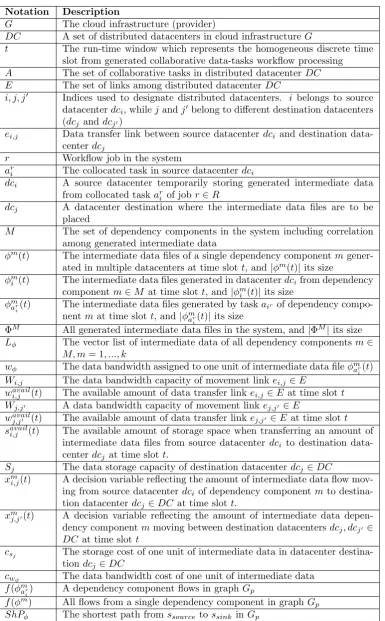
Figure 4.1 shows the representation of the generated directed flow graph Gp = (DCp∪Ap;Ep;u;c)
4.2.2. Greedy heuristic algorithm. A greedy heuristic algorithm has been developed for the minimum cost inter-job intermediate data dependency placement problem through the reduction to the minimum cost of unsplittable multicommodity flow with multiple dependency component sources in flow graph Gp.
Let Sdcj,min be the minimum storage capacity of a destination datacenter dcjp on a network flow graph
Gp, andϕmmax the largest dependency component generated from virtual source datacenter node dc(ϕm)p. As storage resources are scalable in a flow graph Gp acting as a cloud environment, it is realistic to assume that |ϕm
max| ≤Sdcj,minfrom the construction of the flow graphGp. Since the splittable exact algorithm is a relaxation
Fig. 4.1.The generated directed flow graphGp= (DCp∪Ap;Ep;u;c).
components are known a priori, so is their generation order. Hence, the greedy heuristic algorithm adopts an orderly greedy method and starts with the initial placement and works in steps. At the end of each step, it outputs a set of destination datacenters and transfers intermediate data dependencies to that destination data-centers, considering a minimum transfer and storage cost. As the greedy algorithm gives sequential placement solutions, there is no congestion problem on the different dependency components sharing links. Therefore, the greedy algorithm just takes care of the integer dependency component placement (bandwidth capacity is shared between the flows of a single dependency component at time slott) to their destination. The greedy heuristic algorithm execution on a network flow graphGp is provided in the following steps:
Step 1. Let f(ϕm) be the dependency component flow for all dependency intermediate data-task flows ∑
ar i∈A
f(ϕm ar
i) with the minimum total storage cost fromssource tossink. Flowsf(ϕ
m) route dependency
compo-nent commoditiesϕmar
i from different virtual source datacenter nodes connected from source nodessourceto their
destination datacenter nodesdcj(ϕm)
p, the latter being connected with destination nodessink. A set of depen-dency component commodities∑m∈Mϕmare routed tossink in graphGp according to the ascending order of their respective size as dependency component demands: |ϕ1|,|ϕ2|, ...,|ϕk|, withϕ1≥ϕ2≥ϕ3≥...≥ϕk. Let Lϕ= (ϕ1, ϕ2, ..., ϕk) be the dependency component list.
Step 2. Start with the first dependency component by selecting it from list Lϕ. The algorithm scans each dependency component value ϕmar
i(t) inGpto find the possible path which routes the selected dependency
component flowf(ϕm) along each link (dc(ϕm)p, dcj
p) inGpthat satisfies the flow conservation inGpi.e from any
nodesdcp,dc(0)p ∈DCp \ {ssource, ssink}, there is ∑dc(0)p∈DCpf(dcp, dc(0)p) = ∑
dc(0)p∈DCpf(dc(0)p, dcp).
Step 3. For each solution of dependency component flow f(ϕm), find the shortest path notedShP ϕ from ssourcetossinkinGpaccording to the total minimum storage cost, i.e.,c(ShPϕ) =min(dc(ϕm)p,dc
jp)∈Epc(dc(ϕ
m) p, dcjp). Once the shortest path ShPϕ is found, setf(ShPϕ) = ϕ
m and delete iteratively its flow valuef(ϕm ar i).
Define residual capacityures(ssource, ssink) fromssource tossinkin order to decrease the routed flows in graph Gp, i.e., ures(ssource, ssink) =u(ssource, ssink) - f(ShPϕ). Delete the routed dependency componentϕm from listLϕand repeat the sub-procedure of step 2 until all flow valuesf(ϕmar
i) are scanned.
corresponding to graphG.
4.2.3. Time complexity. To build a network flow graphGp for the greedy framework optimization, two steps are needed. The first one consists in assigning each source datacenterdcj ∈DChosting intermediate data to its dependency component nodem∈M, and the second one to each destination datacenterdcj∈DC which is capable of accommodating. The construction ofGptakesO(M+|DC|) for the first step andO(M2+|DC|2)
for the second one. Finally, we analyze the time complexity of the greedy solution which considers mostly the shortest path computing step and the sorting of the list of dependency components. The worst complexity of the sorting computation has a fundamental requirement of O(M2). The shortest path computation step
is more complex and requires computing the distance between all intermediate data dependency components and datacenter destinations. This leads to O(M2× |DC|2) time complexity to consider all combinations or
couples. In summary, the average computational complexity of the proposed greedy heuristic algorithm is O(2M2+|DC|2×(M2+ 1) +M+|DC|) in the worst case.
5. Performance evaluation. This section gives an overview of the simulation, evaluation conditions and settings of the proposed algorithms. A dedicated simulation program has been developed to conduct the performance assessments of the heuristic and compare it with the exact algorithm, random and uniform strategies, named random heuristic and uniform heuristic respectively. The random heuristic strategy randomly selects a datacenter to host the intermediate data until its capacity is exhausted and then selects another one as in default Hadoop scheduler [30] (random capacities and random costs). The uniform heuristic strategy is based on the uniform storage capacity of the distributed datacenter upon intermediate data dependency placement decision (balanced capacities and variable costs). This data placement strategy excludes the storage requirements as in [27, 28, 29, 11]. Subsequently, the performance evaluation overall intends to present relevant comparisons between the solutions found by the greedy heuristic algorithm with the optimal ones found by the exact algorithm in terms of performance metrics like optimality, scalability and convergence time.
5.1. Simulation environment. The heuristic is evaluated through a C++ language implementation. The exact algorithm is implemented with IBM ILOG AMPL and solved optimally using CPLEX. The objective of a numerical evaluation is to quantify the amount of total storage cost saving (objective function) that can be expected when routing intermediate data dependencies through cloud storage infrastructures using the greedy heuristic and exact algorithms. The evaluation also reflects particularly the influence of the number of datacenters, the amount of the routed intermediate data and the dependency parameters on the performance metrics.
The assessment scenarios correspond to a cloud infrastructure consisting of 50 distributed datacenters including source and destination datacenters which are connected to each other randomly. We run the simulation program for 20 random tasks, each one including an amount of a random intermediate data generated per one hour time slot in random adjacency matrix-based DAG, each one having a size ranging from 10 GB to 100 GB [12], including their dependencies that are generated randomly as correlation links in DAG from input to output intermediate data. The latter are assigned randomly to the set of source datacenters in charge of temporarily storing them.
The intra-job dependency is described by a dependency parameter valueαgenerated randomly from range [0, 1] and belonging to each intermediate data-task in the DAG. Value 1 corresponds to a splitting rate of an intermediate data file (a fraction of 1 GB splitting for each file from partial correlation), and the opposite case is represented by value 0. A dependency parameter valueβ is given also that is generated randomly from range [1, 20] which represents the number of clusters randomly grouping intermediate data-tasks. For the inter-job dependency, we set the value of αto 0 from full correlation coupled with dependency parameter valueβ (the case of inter-job dependency is intrinsically related to the intra-job dependency case when the αvalue of the latter converges to 0 and has the same dependency valueβ). On all the carried out experiments, the case when α = 1 and β = 20 are excluded which means that the intermediate data are completely independent. The same dependency parameter value β is assigned to both intra- and inter-job dependencies according to each experiment.
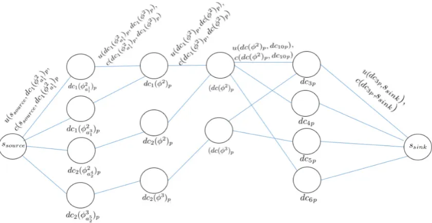
Fig. 5.1. The total storage cost of algorithms exact, greedy, random and uniform heuristics while varying the intermediate data size when the number of datacenters is set to 50.
are randomly drawn from range [1, 10] Gbps [7] with a random transfer cost (in $) ranging from 0 to 0.09. Both storage and transaction costs (in $) of one unit of intermediate data dependency are set within [0.02, 0.04] and [0, 0.09] respectively, in relation to the typical charges in Amazon S33.
5.2. Simulation results. To present the performance of the proposed algorithms regarding their effec-tiveness against comparison strategies solutions, we study the optimality of the exact and greedy heuristic algorithms in terms of the total storage cost ratio, and the results of the scalability and the convergence are reported below.
5.2.1. Impact of the amount of routed intermediate data on algorithms performance. For the specific needs of the simulation, a variation of the amount of intermediate data must be placed from 100 to 1000 GB with an increment of 100 while the number of datacenters DC is set to 50.
To continue to appropriately analyze the simulation, we reflect the concerns of dependency parameter values on the algorithms performance. In this case, each solution found from the execution algorithms is a mean of the results obtained by varying dependency parameters αandβ from range [0, 1] and [1, 20] respectively.
Figure 5.1 depicts the curves of total storage cost delivered by the proposed algorithms and the two other strategies. The figure shows that both greedy heuristic and exact algorithms outperform random heuristic and uniform heuristic strategies in terms of cost. The optimal result obtained by the exact solution reaches a cost of $125 when the amount of placed intermediate data achieves 1000 GB, and the greedy heuristic algorithm achieves a nearly optimal storage cost of $160, which is lower than the costs of the random heuristic and uniform heuristic algorithms (43% and 12% respectively). Clearly, the gap between greedy heuristic and uniform heuristic algorithms is very small since the uniform heuristic is independent of the capacity of the cloud infrastructure, so the cost within the datacenters contrast on the placement decision.
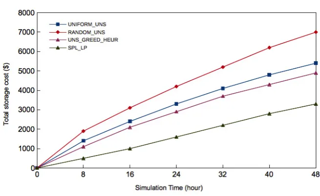
Figure 5.2 depicts the curves of the total storage costs of the algorithms by increasing the simulation time. In this instance, the obtained result of the total storage cost is the aggregation of the previously calculated costs during the same simulation (continuous placement). In addition, the simulation test is conducted for 48h in order to validate the need of the greedy heuristic algorithm and to estimate the probability to have good solutions. The lengthening of simulation at time slot 48 while the number of datacentersDC is set to 50 makes the total storage cost of algorithms greedy heuristic, exact, random heuristic and uniform heuristic to $4900, $3300, $7000 and $5400 respectively. Typically, this means that the cost of greedy heuristic is 10% and 42% less than those of uniform heuristic and random heuristic algorithms, while the result of the exact algorithm
3
Fig. 5.2. Total storage cost of algorithm exact, greedy, random and uniform heuristics when the simulation time is extended to 48h, while the number of datacenters is set to 50.
Fig. 5.3. The amount of intermediate data accumulated per time slot for the proposed algorithms while the number of datacenter ranges from 5 to 50.
as expected remains the best total storage cost. These results show that the uniform capacity constraint on the intermediate data growth directly affects their placement cost as in the case of the uniform heuristic algorithm. In the case of random heuristic algorithm, some datacenters offering the lowest cost are not involved unintentionally (random selection) or of the causes of inability to host data.
The aim of the performed simulation as depicted in Fig. 5.3 is to quantify the amount of intermediate data placed continuously by varying the number of datacenters from 5 to 50 according to capacities. The accumulated intermediate data placement increases with the increase of the number of datacenters for both algorithms, and begins to be stable when cloud infrastructure handles 25 datacenters. Moreover, the amount of intermediate data accumulated by greedy heuristic algorithm is very important over all variations of datacenter instances, more importantly, from 25 to 50, due to the abundance of the cloud infrastructure capacity, i.e. more intermediate data can be placed in the cloud infrastructure. The decline of intermediate data placement from 25 to 50 is due to the fact that the intermediate data routing is limited by data bandwidthwavail
since the bandwidth capacity is shared by all dependency components in the exact algorithm. In contrast, in the greedy heuristic algorithm, the data bandwidth capacity is shared by a single dependency component. However, in the exact algorithm, the amount of placed intermediate data is less in comparison with the greedy solution, because it expands the search space for the exact solution since it is based on the simplex method. Thus, the greedy heuristic algorithm responds well to large datacenter instances for which the exact algorithm has more difficulty to find solutions.
5.2.2. Impact of dependency parameters on the algorithms performance. This section studies the impact of the dependency parametersαandβon the algorithms performance in terms of optimal cost. Since the behavior of the proposed execution algorithms regarding dependency type that are processed are different, a need of a variation of quantitative values is experienced for achieving a useful analysis and allowing optimal cost to the unsplittable placement solutions to be more efficiently identified. On the one hand, interval values are considered to align the types of dependency. On the other hand, values are considered when dependency types diverge. In the following, the assessment scenarios correspond to varying dependency parameters (α,β) pair values. Then, simulation results correspond to pair ranges from (α, β)= (0.1, 18), (0.3, 14), (0.5, 10), (0.7, 6), (0.9, 2). These results are reported on figures below keeping the value of αto 0 and with the same dependency valuesβ for the greedy heuristic algorithm while the number of datacenters is set to 50.
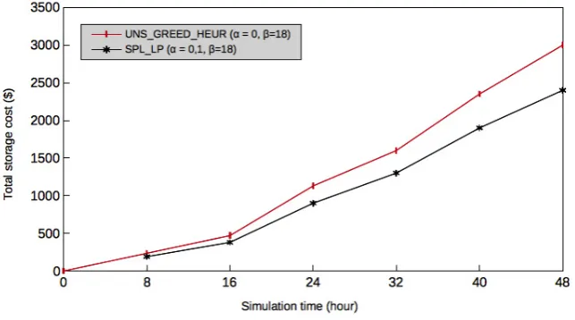
Fig. 5.4. Greedy heuristic versus exact solutions for the total storage cost whenα= 0.1 andβ= 18.
Figure 5.4 depicts the best optimal cost achieved by the objective function for exact and heuristic solutions. The greedy heuristic algorithm performs very well close to the optimal one and achieves a cost of $3000 at time slot 48 that is near to the optimal result of $2400 for the exact algorithm. This is due to the fact that the behavior of the two algorithms have to deal with the aligned correlation α= 0.1 (practically, no amount of intermediate data is splitted with exact, and 0 defaults to the heuristic) with β = 18. Therefore, this has a direct impact on the reduction of the transfer, storage and movement costs for both algorithms.
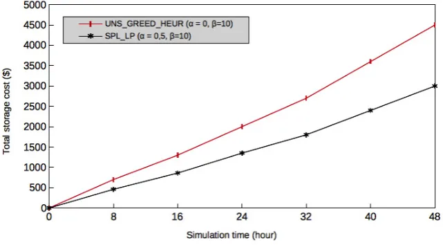
Figures 5.5 and 5.6 depict the second best-case results for the total storage cost which does not exceed $2800, $3000 for the exact algorithm, and $4000, $4500 for the greedy heuristic algorithm at time slot 48. Since, the amount of the dependency movements are marginal to half (α= (0.3, 0.5)) in the exact algorithm, the movement cost is reduced, which reflects the total storage cost. In addition, the heuristic algorithm processes less intermediate data dependencies (10 to 14 clusters). Therefore, it has more chance to find datacenters that have the capacity to allocate those clusters and at the same time offer a better cost.
Fig. 5.5. Greedy heuristic versus exact solutions for the total storage cost whenα= 0.3 andβ= 14.
Fig. 5.6. Greedy heuristic versus exact solutions for the total storage cost whenα= 0.5 andβ= 10.
two algorithms dependents on the amount of intermediate data dependencies. This validates our analysis for the results discussed above (Fig. 5.4, 5.5 and 5.6).
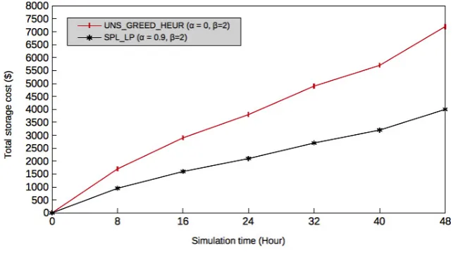
Fig. 5.8 shows the worst case when the highest total storage cost is found for both algorithms. The total storage cost reaches $4200 and $7200 for exact and greedy heuristic algorithms respectively at time slot 48 since the amount of intermediate data dependencies that transit between destination datacenters are significant (α= 0.9) for the exact algorithm (defined by variablexmj,j′(t)). In contrast, the heuristic processes more dependencies
grouped onto two clusters. In addition, the same capacity values were considered for each solution reached with the different values of α and β. Therefore, it has less opportunity to find datacenters than the capacity to allocate those large clusters, and at the same time it offers a better cost. This influences considerably the search for the optimal result which is a real compromise for both algorithms.
Fig. 5.7.Greedy heuristic versus exact solutions for the total storage cost whenα= 0.7 andβ= 6.
Fig. 5.8.Greedy heuristic versus exact solutions for the total storage cost whenα= 0.9 andβ= 2.
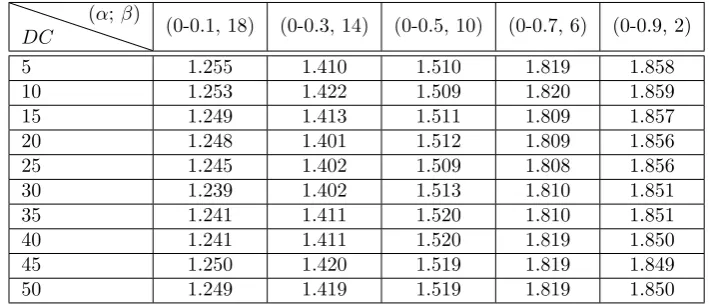
splittable variant of the placement. The cost ratio of the heuristic HEU Risϵ= HEU R
F RAC OP T. The cost ratio of the different curves above (Fig. 5.4 to 5.8 ) is reported in Table 5.2 when the number of datacenters varies from 5 to 50.
One can be see that the cost ratio of the greedy heuristic algorithm is no more than 1.85. Indeed, for simulated instances in the range from 5 to 50 datacenters when dependency parameter pairs (α, β) ={(0.1, 18); (0.3, 14), (0.5, 10)}, the cost ratio of the greedy heuristic algorithm performs closer to the optimal solution and does not exceed 1.25, 1.42 and 1.52 respectively for each pair in fairly adverse conditions.
Table 5.1
Gaps between the greedy heuristic and the exact algorithms in terms of cost ratio.
DC
(α; β)
(0-0.1, 18) (0-0.3, 14) (0-0.5, 10) (0-0.7, 6) (0-0.9, 2)
5 1.255 1.410 1.510 1.819 1.858
10 1.253 1.422 1.509 1.820 1.859
15 1.249 1.413 1.511 1.809 1.857
20 1.248 1.401 1.512 1.809 1.856
25 1.245 1.402 1.509 1.808 1.856
30 1.239 1.402 1.513 1.810 1.851
35 1.241 1.411 1.520 1.810 1.851
40 1.241 1.411 1.520 1.819 1.850
45 1.250 1.420 1.519 1.819 1.849
50 1.249 1.419 1.519 1.819 1.850
restrictions. Indeed, each proposed algorithm responds differently to the dependency requirements as well. A special cases are also considered which are not reported on Table 5.2, when dependency parameter pairs are set from a range of (α, β) = (0.1, 1), (0.1, 2), (0.9, 19), (0.9, 18). These parameter values are the most extreme and contradictory cases, in the sense that for dependency pairs (0.1, 1) and (0.1, 2), the exact algorithm finds a solution with an adjustment of time (beyond the days) but could not find an optimal solution, and for the latter cases (0.9, 19) and (0.9, 18), this does not reflect the correlation-type of intra-job dependency.
We conclude that the cost ratio of the greedy algorithm depends on the value of the dependency parameters and the amount of intermediate data that increase at each time slot. In the two cases, where the dependency parameters nearly correlate (α, β) = {(0.1, 18); (0.3, 14), (0.5, 10)}, the cost ratio is more profitable. This means that the two proposed algorithms reacted well to these dependency value requirements. However, the cost ratio of the greedy algorithm that is reported in Table 5.2 increases as dependency parameters deviate (α, β) ={(0.7, 6); (0.9, 2)}.
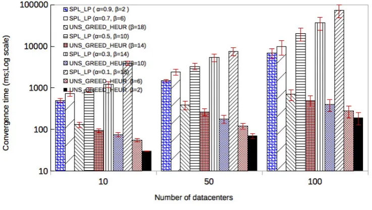
5.2.3. Convergence time of the proposed algorithms. To pursue the extensive experiments, we evaluate the effectiveness of the proposed algorithms and compare them in terms of scalability and convergence time from input parameters. For the comparison, we extend the simulation by varying the number of datacenters from 10 to 100 and by setting the amount of routed intermediate data from 100 GB to 1000 GB. Obviously, the values of the dependency parameters must also vary in order to better understand the behavior of the execution time of the proposed algorithms as regard to the dependencies. Thus, the value of dependency parameters is set as specified in Sec. 5.2.2. Algorithm running times are recorded as follows.
First, the execution time of the greedy algorithm solves the placement problem one to four orders of mag-nitude faster than the exact solution. However, the exact algorithm solves the NP-hard problem in exponential time for large instances since a part to solve the simplex-based LP method takes much time, particularly for αvalues between 0.1 and 0.5 because the intermediate data splitting parameters are less tolerated throughout their placement. Furthermore, the values of dependency parameters correlate with the continuous amount of intermediate data bounded by a discrete quantity. Not surprisingly, greedy heuristic is much easier to solve than the exact algorithm.
Indeed, Fig. 5.9 shows the best convergence time for each of the proposed algorithms.
Fig. 5.9.Time execution comparison between greedy heuristic and exact algorithms for different datacenter size when varying the amount of generated intermediate data (|ΦM|= 100 GB).
Fig. 5.10.Time execution comparison between greedy heuristic and exact algorithms for different datacenter size when varying the amount of generated intermediate data (|ΦM|= 500 GB).
Figures 5.10 and 5.11 show the worst cases for the exact algorithm. Then, the time needed for convergence grows mainly for an amount of placed intermediate data. These amount varies between 500 GB and 1000 GB for the simulated scenarios from 50 to 100 datacenters while the time running the greedy heuristic remains very fast to find solutions with a convergence time improvement ratio in range [101,103] as compared to the exact
Fig. 5.11.Time execution comparison between greedy heuristic and exact algorithms for different datacenter size when varying the amount of generated intermediate data (|ΦM|= 1000 GB).
Particularly, this corresponds to values of α that vary from 0.1 to 0.5, where the exact algorithm exceeds a running time of one minute as shown in Fig. 5.10.
The convergence time increases with the number of datacenters as well as slightly less with the amount of intermediate data (see Fig. 5.11). As a matter of fact, the capacity of bandwidth is limited to 10 GB for data transfer, but with more transfer links through the growth of the number of datacenters.
The gap between the algorithms is in range [102,104] with an improvement factor in favor of the greedy
heuristic.
As expected for the exact algorithm that was built upon the simplex method (which is based on the number of intermediate data to be fractionated and this is done for each iteration as the scale of the datacenter and links between them, meaning that the separation procedure is generally not polynomial) and even with the use of a set of dependency constraint values to limit the convex hull problem to find the optimal solution faster that goes beyond 500 GB for100 datacenters, the convergence time remains widely slow at about 7 minutes.
In conclusion, the execution time of the proposed algorithms depends mostly on the cloud infrastructure topology, and slightly less on the amount of intermediate data dependencies for the exact algorithm. Besides, the change in dependency parameter values influences largely the exact algorithm performance and much less the greedy heuristic. This validates the motivation for the use of a heuristic approach to find solutions faster even if there are bound to be approximated (as reported in Table 5.2).
data for larger instances, we developed a heuristic based on a greedy optimization framework, this, solves the problem in very fast time, making an assumption of an optimal fractional solution. The evaluation tests show that the greedy heuristic algorithm performs closer to the exact formulation solution (in the case of converged correlations), and boots higher performance as compare to other state of the art strategies. We evaluated also the convergence time of the proposed algorithms. It is improved by several orders of magnitude for the greedy heuristic algorithm compared to the exact algorithm, while making possible to solve large cloud infrastructures in a reasonable time.
REFERENCES
[1] P. Kolman,A note on the greedy algorithm for the unsplittable flow problem, in Information Processing Letters Elsevier, vol. 88, no 3, (2003), pp. 101–105.
[2] P. Krysta,Greedy approximation via duality for packing, combinatorial auctions and routing, in International Symposium on Mathematical Foundations of Computer Science (Springer 2005), pp. 615–627.
[3] Belaidouni, Meriema and Ben-Ameur, Walid,On the minimum cost multiple-source unsplittable flow problem, RAIRO-Operations Research , 41(3), (2007), pp. 253-273
[4] A. Chakrabarti, C. Chekuri, A. Gupta, and A. Kumar,Approximation algorithms for the unsplittable flow problem, Algorithmica, (2007), vol. 47, no 1, pp. 53-78.
[5] H. Pirsiavash, D. Ramanan, and C. C. Fowlkes,Globally-optimal greedy algorithms for tracking a variable number of objects, Computer Vision and Pattern Recognition (CVPR), 2011 IEEE Conference on. IEEE, (2011). pp. 1201-1208. [6] Q. Xia, W. Liang, and Z. Xu, The operational cost minimization in distributed clouds via community-aware user data
placements of social networks, Computer Networks (2017), vol. 112, pp. 263-278.
[7] Q. Xia, Z. Xu, W. Liang, and A. Y. Zomaya,Collaboration-and fairness-aware big data management in distributed clouds, in IEEE Transactions on Parallel and Distributed Systems (2016), 27(7), pp. 1941-1953.
[8] P. Agrawal, D. Kifer, and C. Olston,Scheduling shared scans of large data files, Proceedings of the VLDB Endowment (2008), vol. 1, no 1, p. 958-969.
[9] T. Nykiel, M. Potamias, C. Mishra, G. Kollios, and N. Koudas,MRShare: sharing across multiple queries in MapReduce, Proceedings of the VLDB Endowment 3.1-2 (2010), pp. 494-505.
[10] Q. Sun, M. Romanus, T. Jin, H. Yu, P. T. Bremer, S. Petruzza, ... and M. Parashar, In-staging data placement for asynchronous coupling of task-based scientific workflows, in Extreme Scale Programming Models and Middlewar (ESPM2), International Workshop on (2016), pp. 2-9. IEEE.
[11] Q. Zhao, C. Xiong, X. Zhao, C. Yu, and J. Xiao,A data placement strategy for data-intensive scientific workflows in cloud. In Cluster, Cloud and Grid Computing (CCGrid), 2015 15th IEEE/ACM International Symposium on (2015), pp. 928-934. IEEE.
[12] M. Ebrahimi, A. Mohan, A. Kashlev, S. Lu,BDAP: a big data placement strategy for cloud-Based scientific workflows. In Big Data Computing Service and Applications (BigDataService), IEEE First International Conference on (2015), pp. 105-114. IEEE
[13] R. Vilaa, R. Oliveira, J. Pereira,A correlation-aware data placement strategy for key-value stores, in IFIP International Conference on Distributed Applications and Interoperable Systems (2011), pp. 214-227. Springer Berlin Heidelberg. [14] Q. Zhao, C. Xiong, P. Wang,Heuristic Data Placement for Data-Intensive Applications in Heterogeneous Cloud, in Journal
of Electrical and Computer Engineering, 2016.
[15] Asano, Y.,Experimental Evaluation of Approximation Algorithms for the Minimum Cost Multiple-source Unsplittable Flow Problem, In ICALP Satellite Workshops (2000), pp. 111-122
[16] D. Warneke, O. Kao, Nephele: efficient parallel data processing in the cloud, in Proceedings of the 2nd workshop on many-task computing on grids and supercomputers. ACM (2009), pp. 8.
[17] X. Liu, A. Datta,Towards intelligent data placement for scientific workflows in collaborative cloud environment, in Parallel and Distributed Processing Workshops and Phd Forum (IPDPSW), 2011 IEEE International Symposium on. IEEE (2011), pp. 1052-1061.
[18] Z. Wu, X. Liu, Z. Ni, D. Yuan, and Y. Yang,A market-oriented hierarchical scheduling strategy in cloud workflow systems, The Journal of Supercomputing (2013), vol. 63, no 1, pp. 256-293.
[19] X. Liu, Z. Ni, Z. Wu, D. Yuan, J. Chen, and Y. Yang,A novel general framework for automatic and cost-effective handling of recoverable temporal violations in scientific workflow systems, in Journal of Systems and Software (2011), vol. 84, no 3, pp. 492-509.
[20] D. Wang, and J. Liu,Optimizing big data processing performance in the public cloud: opportunities and approaches, IEEE network (2015), vol. 29, no 5, pp. 31-35.
[21] J. Jin, J. Luo, A. Song, F. Dong, and R. Xiong,Bar: An efficient data locality driven task scheduling algorithm for cloud computing, in Proceedings of the 2011 11th IEEE/ACM International Symposium on Cluster, Cloud and Grid Computing. IEEE Computer Society (2011), pp. 295-304.
[22] L. Kaufman, and P. J. Rousseeuw,Finding groups in data: an introduction to cluster analysis, vol. 344, (2009) John Wiley & Sons.
[24] V. P. Anuradha, and D. Sumathi,A survey on resource allocation strategies in cloud computing, in Information Commu-nication and Embedded Systems (ICICES), 2014 International Conference on (2014), IEEE, 2014. pp. 1-7.
[25] D. Ardagna, G Casale, M. Ciavotta, J. F. Prez, and W. Wang, Quality-of-service in cloud computing: modeling techniques and their applications, Journal of Internet Services and Applications (2014), vol. 5, no 1, pp. 11.
[26] Z. Xu, and W. Liang,Operational cost minimization of distributed data centers through the provision of fair request rate allocations while meeting different user SLAs, Computer Networks (2015), vol. 83, pp. 59-75.
[27] S. Agarwala, D. Jadav, and L. A. Bathen,iCostale: adaptive cost optimization for storage clouds, in Cloud Computing (CLOUD), 2011 IEEE International Conference on. IEEE (2011). pp. 436-443.
[28] D. Yuan, Y. Yang, X. Liu, G. Zhang, and J. Chen,A data dependency based strategy for intermediate data storage in scientific cloud workflow systems, in Concurrency and Computation: Practice and Experience (2012), vol. 24, no 9, pp. 956-976.
[29] X. Ren, P. London, J. Ziani, and A. Wierman,Joint data purchasing and data placement in a geo-distributed data market, ACM SIGMETRICS Performance Evaluation Review. ACM (2016). pp. 383-384.
[30] T. da Silva Morais, Joint data purchasing and data placement in a geo-distributed data marketSurvey on frameworks for distributed computing: Hadoop, Spark and Storm, in Proceedings of the 10th Doctoral Symposium in Informatics Engineering-DSIE (2015). Vol. 15.
[31] A. Dalvandi, M. Gurusamy, and K. C. Chua,Application scheduling, placement, and routing for power efficiency in cloud data centers, in IEEE Transactions on Parallel and Distributed Systems (2017). 28, no. 4 pp. 947-960.
[32] A. Gawanmeh, S. Parvin and A. Alwadi,A Genetic Algorithmic method for scheduling optimization in cloud computing services, in Arabian Journal for Science and Engineering (2017), pp. 1-10.
[33] B. A. Rao and L. V. Vahini,Efficient scheduling of scientific workflows using multiple site awareness big data management in cloud, in International Journal of Scientific Research in Computer Science, Engineering and Information Technology (2018). Volume 3 — Issue 1 — ISSN : 2456-3307.
[34] M. H. Ferdausa, M. Murshedb, N Rodrigo Calheirosc and R. Buyyac, An algorithm for network and data-aware placement of multi-tier applications in cloud data centers, in Journal of Network and Computer Applications (2017), vol. 98, pp. 65-83.
[35] A. M Manasrah and H. Ba Ali,Workflow Scheduling Using Hybrid GA-PSO Algorithm in Cloud Computing, in Wireless Communications and Mobile Computing (2018), vol. 2018.
[36] N. Anwar and H. Deng,A Hybrid Metaheuristic for Multi-Objective Scientific Workflow Scheduling in a Cloud Environment, in Applied Sciences (2018), vol. 8, no 4, pp. 538.
[37] H. Arabnejad and J. G. Barbosa,List scheduling algorithm for heterogeneous systems by an optimistic cost table, in IEEE Transactions on Parallel and Distributed Systems (2014), vol. 25, no 3, pp. 682-694.
[38] M. Abdullahi and M. A. Ngadi,Symbiotic Organism Search optimization based task scheduling in cloud computing envi-ronment, in Future Generation Computer Systems (2016), vol. 56, p. 640-650.
Edited by: Sasko Ristov
Received: Feb 14, 2018