A Review of Methods for Point and Interval Estimation of Population Size in Capture-Recapture Studies

A Review of Methods for Point and Interval Estimation of Population Size in

Capture-Recapture Studies

Carlo Cosenza

Lynn Eudey, PhD

Joshua Kerr, PhD

Bruce Trumbo, PhD

Abstract

Estimates of population size in a classical capture-recapture experiment are obtained by method of moments and maximum likelihood estimation. Exact confidence intervals using the hypergeometric distribution (the general method) and approximate confidence intervals using the normal approximation and separately, the binomial approximation are illustrated. Estimates of coverage probabilities are explored using the hypergeometric distribution for the general method and for both approximate methods. Bayesian methods of interval estimation are also illustrated. The computer software R is used to do the intensive computation and make figures. R-code for the methods is provided in text boxes. The capture-recapture study provides a unique setting in which to explore both traditional and Bayesian estimation methods using a discrete distribution with a discrete prior.

Key Words:

1. Introduction

In the first edition (1950) of his famous introductory probability book, Feller introduces estimation of the size of a closed population, fish in a lake, by using the capture-recapture (or mark-recapture) method to illustrate the hypergeometric distribution. In the third edition, Feller (1968) mentions in a footnote, that in 1950 he had not realized the widespread practical use of the method. Since then examples very similar to Feller's have continued to appear in probability books, while researchers in many fields have developed elaborations of the method to apply in a wide variety of practical problems. Capture-recapture has census, economic, epidemiological, medical, and social sciences applications. (Refer to the review articles by Chao (2001) and Chao, et al. (2001).)

Our purpose here is to take advantage of relatively easy computation in R statistical software to review and illustrate a variety of methods of point and interval estimation of population size. The use of R software has become very popular and is widely used in both academic and commercial applications. (See the New York Times article by Vance, 2009.)The computation involved in the methods is easily programed in R and R-code is provided in text boxes.

The remaining sections of this paper are organized to introduce the basic capture-recapture

method with its assumptions, and to discuss related methods of estimation.

Specifically, we illustrate method of moments and maximum likelihood point estimation, and develop confidence intervals using the hypergeometric distribution, as well as using normal and binomial approximations. In addition, we explore Bayesian probability intervals with flat and mildly informative priors. Because the hypergeometric likelihood function is discrete, and because it is feasible to select discrete prior distributions, it is possible to use the elementary discrete version of Bayes' Theorem to discuss Bayesian inference.

2. The Capture-Recapture Method and Method-of-Moments Estimation

Some animal species and populations are at risk because of pollution, climate change, loss of habitat, and other environmental hazards. Scientists who seek an objective view of how serious these risks are and how damage might be reversed often need to estimate the size of a population.

As an illustration, suppose we want to know approximately how many fish of a certain kind are in a lake. Suppose that the population had been depleted and we hope remedial action over the last couple of years has helped with re-population. We need an indirect method of estimation. One experimental method that sometimes gives useful results involves sampling in two stages (capture-recapture).

2.1. Two-step experiment. A capture-recapture study is conducted so that hypergeometric distributions

can be used to estimate the population size (let represent population size). Suppose we go fishing with a net at random places around the lake in which we want to estimate .

Capture: At the first stage, we randomly sample (without replacement) r = 1100 fish of the size and species of concern, and we mark them with small red tags. We will call these fish "red'' and the rest of the fish (of the species of interest) in the lake "white.''

Recapture: Later, we sample without replacement k = 900 fish at random from the lake, and we note the number X of red fish among the 900.

Often r = k, but we choose different values to avoid confusion of r and k in numerical examples. Also, our notation is chosen to make a clear distinction among the unknown population parameter , the known design parameters r and k, and the random number X of red fish seen upon recapture. In summary, r = number of fish initially tagged red, k = the number of fish (both red and white) resampled (recaptured), X = number of red fish in the recapture sample, and  = total fish population size.

2.2 The hypergeometric distribution. Let X = number of successes in a random sample drawn of size k

drawn without replacement from a population of size  with r successes and  - r failures. Then X has a hypergeometric distribution with probability mass function:

ℎ( | ) =

−

− _{, for = 0, 1, 2, … , min ( , )}

Where = !

2.3. Estimation by the method of moments. For illustration, suppose X = 99. Then we have two equations for the proportion of red fish in the lake at recapture:

The true proportion is r/ and the statistic X/khas expectation, E(X/k) = r/ Setting X/kr/ , we have the estimate T = rk/Xof In our numerical example, the point estimate of the population size is T = 1100(900)/99 = 10000. An estimate found by setting a statistic equal to its expected value (first moment) is often called a method-of-moments estimator (MME).

Sometimes MMEs are unbiased, but the nonlinear arithmetic used in solving for T leads to E(T) > , not E(T) = A formal proof is beyond the scope of this paper, but we notice that sinceX has a hypergeometric distribution (in which we observe the number of red fish in sampling k = 900 fish from a population with r = 1100 red fish and – r white fish) we can compute this exactly in R. Then, usinga quick simulation in R (shown below), in which this recapture procedure is repeated m = 100,000 times from a population with = 10,000. In one run, we obtained E(T) 10,083.22 and would estimate population size as 10,083 fish. (Based on our experiment, we are confident of the slight upward bias because the margin of error for this simulation is roughly only about 6 fish.)

m = 100000; k = 900; r = 1100; tau = 10000 x = rhyper(m, r, tau - r, k); t = k*r/x; mean(t)

The estimator T (used in the previous example) is referred to as the Lincoln-Peterson estimator and is asymptotically unbiased (Peterson, 1896; Lincoln, 1930). The small biaswe observed here (less than 1%), while worth noting, is not enough to make T a bad estimate of for many practical

purposes. However, for small samples the Chapman estimator, = ( )( )– 1, is preferred because it has less bias (Chapman, 1951).

2.4. Assumptions. The usefulness of T as an estimate of depends on some assumptions. We assume

that samples at the capture and recapture stages are two independent random samples from the same population. In particular, the estimate would not be valid if fish had been born, had died, had immigrated, or had emigrated between times the two samples were taken. Thus the word later at the beginning of the second bullet is a little tricky. We have to allow enough time for the marked fish to distribute themselves randomly through the population before the second sample is taken, but not so long that the population will have changed.

Also, we assume that fish marked at the first sampling are neither more nor less likely to be chosen at the second. This is worth mentioning because in some applications it has been observed that animals, having been trapped once, may become “trap-shy” (they felt uncomfortable being caught) or “trap-happy” (they enjoyed the attention or the bait).

Other authors have addressed modifications of the basic capture-recapture method to detect and correct for departures from these assumptions. Additionally, some more advanced schemes incorporate information from several recaptures.

3. Maximum Likelihood Estimation of the Population Size

Maximum likelihood estimation (MLE) is very widely used. Methods of mathematical statistics show that in many applications MLEs have desirable properties. We begin with an example that is similar to estimating the number of fish in a lake, but much simpler.

3.1. Urn-sampling distributions. Suppose two balls are chosen at random and without replacement

Then Table 1 shows hypergeometric distributions of Y for three such urns. For example, in R the

distribution for Urn C can be computed asdhyper(0:2, 9, 91, 2).

Table 1.Distributions of the probability of drawing Y red balls when two balls are sampled from three urns A, B, and C with nine red balls and different numbers of white balls (Because of rounding, some column totals are not exactly one.)

Suppose one of the urns is chosen at random and we are trying to guess which urn. If we are told the value ofY (the number of red balls seen among two balls drawn from this urn) then intuitively this information is a big help in guessing whether the urn is the one with a total of 10, 20, or 100 balls. If

Y = 1, then a simple application of the principle of maximum likelihood would lead us to select Urn B. Specifically, reading across rows of Table 1, we choose Urn B because observed outcome Y = 1 has the largest likelihood for that urn. Similarly, if Y = 2, we choose Urn A; and if Y = 0, we choose Urn C. Now we use a slightly more complicated version of the same idea to estimate the number of fish in the lake.

3.2. Maximum likelihood estimate of population size. Intuitively, we see that the more red fish we

recapture the smaller the number of fish we guess are in the lake. At one extreme, if all of the recaptured fish were red, we would suppose there must be only about 1100 fish in the lake. By contrast, if very few of the recaptured fish were red, we would suppose the population size to be quite large.

In the capture-recapture example, we imagine a huge number of urns (lakes). All have r = 1100 red fish (marked fish), but the number of white fish might range from w = 0 to some very large number. Holding constant the numbers r = 1100, k = 900, and X = 99, we letw vary over a wide range of values (here = r + w). Then we pick the value of that makes the likelihood of recapturing exactly 99 fish greatest.

More analytically, if r, k, and are known, then the probability mass function for X is shown in section 2.2.

However, once we have observed X = x, then h(x | ) may be considered a function of and is denoted ( | ). In this case, ( | )is called the likelihood function of , and the maximum likelihood estimate (MLE) of is the value T of for which ( | )is maximized. This is equivalent to scanning across a row of Table 1, corresponding to an observed value, to find distribution with the maximum probability value.

Specifically, in our example we want to find the population size that maximizes

( |99).Because of the discreteness of , we cannot use methods of calculus to find the MLE. One

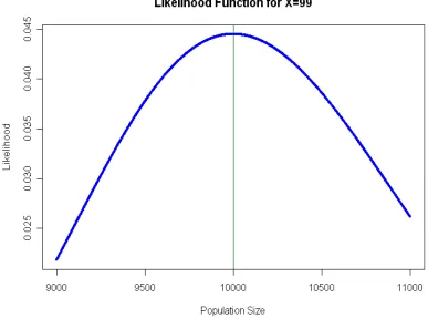
approach is to use R to look at many possible values of and search for the value of  that maximizes the likelihood function. This is called a grid search. The answer is that the MLE is T = 10,000. Figure 1 illustrates the likelihood curve and the location of its maximum.

tau = 9000:11000; r = 1100; k = 900; x = 99 like = dhyper(x, r, tau - r, k)

tau[like == max(like)]

Notes: (1) Theoretically, the value T = 9,999 ties 10,000 to maximize L, but the computation is intensive and the results for L(9,999 | 99) and L(10,000 | 99) incorrectly differ in the 16th decimal place in our version of R.

Urn A (r = 9, w = 1) B (r = 9, w = 11) C (r = 9, w = 91)

P(Y = 0) 0.000 0.289 0.827

P(Y = 1) 0.200 0.521 0.165

(2) The MLE can also be found analytically: Feller (1968) points out that, after some algebra:

( | )

( = 1| )=

− − +

− − −

from which one can deduce that the ratio is greater or smaller than unity according as x<rk or x>rk. So that ( | ) ascends to a maximum at the integer ceiling of rk/x and then descends. In our example, these two products can be equal, so the MLE of  can be taken as either 9,999 or 10,000, and we choose the latter.

It turns out that, for the capture-recapture problem, the two methods (MME and MLE) of estimating are numerically equal. It is nice to know that two frequently satisfactory methods of estimation agree. However, T = 10,000 is only an estimate, and in practice we would like to know is how close this estimate might be to the right answer.

It seems intuitively clear that we are not going to narrow the population size down to the nearest fish because it is not hard to imagine getting 110 or 90 marked fish on recapture instead of 99, and thus estimating as 9,000 or 11,000 instead of 10,000. In following sections we look at several ways to get interval estimates of the population size .

Figure 1. Likelihood function of population size for X = 99 red fish in a recapture sample of

size 900 with 1100 red fish in the population of unknown size . The MLE of is 10,000. The

"curve" actually consists of 2001 discrete and closely-spaced dots

4. Confidence Intervals for Population Size

With a little trial and error, looking at round numbers, we see that = 8390 must be about at

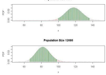
the lower end of the range of believable values because P{X 99 | = 8390}  2.5%. (see the top panel in Figure 2). In R, phyper(99, 1100, 8390 - 1100, 900)returns 0.0248.Similarly, = 12,080 is a very large value of the population size in these circumstances because P{X 99 | = 12,080}  2.5% (bottom plot in Figure 2). So, roughly speaking, it seems reasonable to say that must lie between 8390 and 12,080. This is an approximate 95% confidence interval for . This confidence interval is based on the hypergeometric distribution alone, and thus might be called an exact confidence interval (one not based on an approximation of the hypergeometric distribution).

Figure 2: Illustration of approximate extremes in believable population sizes given that 99 red

fish were recaptured. Heavy green bars represent the central 95% of the probability in each plot.

4.1. A general method for confidence intervals. Because hypergeometric distributions are discrete,

we cannot generally cut off exactly 2.5% from a tail, but by using grid searches we can come a little closer than shown in Figure 2. The R code below comes as close as possible to putting 2.5% in each tail without exceeding 2.5%. The resulting 95% confidence interval is (8392, 12,086).

tau = 5000:13000; x = 99

lwr = max(tau[phyper(x+.5, r, tau-r, k) <=.025]); lwr upr = min(tau[phyper(x-.5,r,tau-r,k) > .975]); upr

Consequently, for a horizontal line at the observed value of X, the blue lower and upper boundaries determine an approximate 95% confidence interval (no more than 2.5% error probability on each side).

Figure 3. The green shaded region corresponds to 95% confidence. When X = 99, the confidence

interval for is (8392, 12,086). The vertical red lines at the ends of the confidence intervals

correspond (roughly) to the two distributions in Figure 2, where thick green bars lie within the green-shaded band in this figure.

4.2. Confidence intervals based on normal approximations. For large andr/ and k/ not too close

to 0 or 1, as in our example, the hypergeometric random variable, X, is approximately normal. Furthermore,

= E(X) = k(r/ ) and 2 = Var(X) = k(r/ )(1 – r/ ( – k)/( – 1) ,

where the factor in brackets expresses the decrease in variability due to sampling without replacement (as opposed to sampling with replacement as in a binomial model).

Thus, an approximate test of the null hypothesis H0: = 0 against the two-sided alternative, can be formulated in terms of the test statistic Z = (X – rk 0) / 0, where 0is with replaced by

0. This method is implicit in a normal approximation recommended by Feller(1968). (Because Z is expressed in terms of 1/ 0 some authors speak of a test on the reciprocal of the sample size.)

t.0 = 5000:13000

sg = sqrt(k*(r/t.0)*(1 - r/t.0)*((t.0 - k)/(t.0 - 1))) Z = (99 - r*k/t.0)/sg; acc = t.0[abs(Z) <= 1.96] min(acc); max(acc)

Recall that the 95% confidence interval from the general method based on the hypergeometric distribution is (8392, 12,086), of length 3694. The current interval from the normal approximation is wholly contained in the one from the general method. How well the normal approximation works depends on the design parameters and the value of X. Often, intervals based on the normal approximation are shorter just because they can place exactly 2.5% of the probability under the normal curve in each tail. Of course, all other things being equal, shorter intervals are preferable, but there is no free lunch. The potential difficulty is that the shorter intervals from the normal approximation may not actually achieve the claimed 95% coverage probability. After looking at another approximation here, we investigate coverage probabilities in the next section.

4.3. Confidence intervals based on binomial approximations. The proportion p = X/k of red fish in

the resample estimates the proportion of red fish in the lake. Then the estimate T = rk/X of becomesT = r/p. Of course, X has a hypergeometric distribution, but for large (say, at least ten

times as large as k), X is approximately BINOM(k, ). An essential difference between the

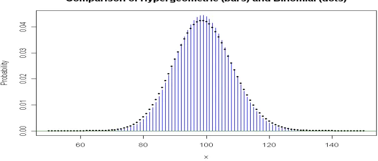
hypergeometric and the approximating binomial is that the former has smaller variance by a factor of ( – k)/( – 1). Figure 4compares the hypergeometric distribution based on choosing 900 balls from an urn with 1100 red balls among 10,000 with BINOM(900, 0.11).

Furthermore, a traditional approximate 95% confidence interval for the binomial proportion is p1.96D, where D = [p(1 – p)/k]1/2. If we trust this interval, then we can use its endpoints pL and

pU to get endpoints of a 95% confidence L = r/pU and U = r/pLfor . However, as shown in Brown,

Cai, and Dasgupta (2001), such intervals for may not have 95% probability of covering the true value of . They require Z = (X – k )/ to be approximately standard normal and for =

( )

to be well approximated by D. Roughly speaking, these traditional intervals may have

much less coverage than the nominal coverage probability if k is too small or is too far from 1/2. The 95% intervals can be somewhat improved by using X' = X + 2 and k' = k + 4; this adjustment should be ignored only when its numerical effects are negligible.

In our example X' = 101 and k' = 904, yields the adjusted point estimate 0.112 and interval (8317, 12063) as an adjusted, but still approximate 95% confidence interval for , according to the R code shown below. This interval has length 3746. Thus for our example, this type of interval gives a longer result than either of the two methods we have considered previously. This type of interval using binomial approximation is much simpler to compute than the other two, and is widely used in elementary discussions of the capture-recapture method. [However, we see no reason to consider using the still longer, unadjusted interval (8433, 12282).]

Figure 4. The binomial distribution with 99 trials and success probability 0.11 is a reasonably close approximation to the hypergeometric distribution of the number X of red balls among 99 chosen without replacement from a population with 1100 red balls among 10,000. The distributions have the same mean, but the hypergeometric distribution has slightly smaller variance.

5. Coverage Probabilities of Confidence Intervals

The confidence intervals we have considered in the previous section aim to have 95% coverage probabilities. For a given design parameters r and k, we may observe one of the possible values of the random variable X= 0, 1, 2, ...,min (r,k). According to whatever method of making confidence intervals is used, an observed value x of X produces a confidence interval, which either covers (includes) the true value of the population parameter , or not. Now suppose the true value of is known. Then the hypergeometric distribution of X is known, and from that we can find the probability that the resulting confidence interval covers . Ideally, this probability would always be 95%, but that is not always so in practice.

5.1. Coverage probabilities for the general method. In our example, we begin by generating the

lower and upper endpoints of the confidence intervals corresponding to the possible values of X. The first lines of R code just below generate the various confidence intervals. The first three columns in

Table 2, show x, the lower confidence limit, and the upper confidence limit, respectively. Next, suppose

we know = 10,000. Another line of code determines whether the interval does (1), or does not (0), contain this value of , as shown in the next column of the table. For brevity, Table 2 shows rows only for selected values ofx. The last line of code essentially produces the table, which we have formatted for publication.

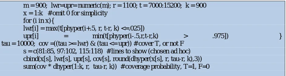
m = 900; lwr=upr= numeric(m); r = 1100; t = 7000:15200; k = 900

x = 1:k # omit 0 for simplicity for (i in x){

lwr[i] = max(t[phyper(i+.5, r, t-r, k) <=.025])

upr[i] = min(t[phyper(i-.5,r,t-r,k) > .975]) }

tau = 10000; cov =((tau >= lwr) & (tau <= upr)) # cover T, or not F s = c(81:85, 97:102, 115:118) # lines to show (chosen ad hoc) cbind(x[s], lwr[s], upr[s], cov[s], round(dhyper(x[s], r, tau-r, k),3)) sum(cov * dhyper(1:k, r, tau-r, k)) # coverage probability, T=1, F=0

x lower upper covprob

...

81 10029 15147 0 0.006 82 9920 14938 1 0.007 83 9815 14735 1 0.009 84 9711 14537 1 0.011 85 9610 14344 1 0.013 ...

97 8546 12366 1 0.044 98 8468 12224 1 0.044 99 8392 12086 1 0.045 100 8317 11951 1 0.044 101 8244 11819 1 0.043 102 8171 11689 1 0.042 ...

115 7338 10227 1 0.009 116 7281 10129 1 0.007 117 7225 10033 1 0.006 118 7170 9938 0 0.005 ...

Table 2. The first three columns of the table show values xand the lower and upper limits of the

intervals they generate according to the general method. Based on = 10,000 the last two

columns indicate whether the interval covers , and P{X = x | = 10,000}. Only selected rows

are shown. The total probability in the boldface region where the intervals cover , is P{82 X

117} = 95.56%.

Notice that a relatively slight change in the value of can make a "sudden" change in the coverage probability. For example, changing from 10,028 to 10,029 would cause the interval for

X = 81 now to cover , and thus include in the sum for the coverage probability the value P{X = 81}, which would itself change only very slightly owing to this change in . By contrast, a change in from 10,032 to 10,034 would cause P{X = 117} to be lost from the sum.

(Because a capture-recapture design has two design parameters r and k, a thorough investigation of coverage probabilities is beyond the scope of the current article.)

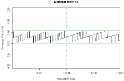
Figure 5.Coverage probabilities of general-method confidence intervals with nominal coverage 95%, for values of t between 8000 and 12,000. For this relatively conservative method, coverage probabilities range between 95.03% and 96.18%. The coverage probability found in Table 2 is shown at the dotted vertical line.

5.3. Coverage probabilities for approximate methods. By constructing confidence intervals

according to the normal approximation method of Section 4 for each possible value of X, comparing the results with various values of to check for coverage, and using hypergeometric probabilities for X, we can obtain a graph of coverage probabilities for the normal approximation method similar to Figure 5.

Figure 6. Coverage probabilities of confidence intervals for obtained using normal

approximations. These intervals tend to be shorter than those in Figure 5. Accordingly coverage probabilities range between 94.3% and 95.6%.

Similar computations for intervals obtained using the binomial approximation method lead to the coverage probabilities illustrated in Figure 7. Because these intervals are considerably longer than those shown in Figures 5 and 6, coverage probabilities for the cases plotted are nearer 96% than 95%.

A thorough investigation of coverage probabilities for these approximate methods for various design parameters r and k and more extended ranges of possible population sizes is beyond the scope of this paper.

Figure 7. Coverage probabilities of confidence intervals for obtained using binomial

6. Bayesian Probability Intervals

The design of many experiments flows from some previous knowledge about unknown parameters. Bayesian analysis requires that previous knowledge be formalized. A population parameter is viewed as random variables having a prior distribution. Then using Bayes’ Theorem, information from the prior distribution and data are combined to give a posterior distribution. Point and interval estimates of the parameter are based on the posterior distribution.

6.1. Three Urns Revisited:

We return once more to the three urns of Table 1. As before, suppose a friend selects one of the three urns. In order to help you guess which urn it is, you are permitted to sample two balls at random from it. If you believe your friend has selected one of the three urns at random, you start with the prior distribution (1/3, 1/3, 1/3) for the three urns A, B, and C.

However, after you draw two balls from the urn presented to you, you have data to use together with your prior distribution. Suppose you get Y = 1 red ball in the two balls you sample. Bayes' Theorem shows how to do the required probability computation. For example, defining event DP(Y =1), we have

( | = 1) = ( | ) = ( ∩ )

( ) =

( ) ( | )

( ) =

0.0667

0.2953= 0.226

where the denominator is computed as

( = 1) = ( ) = ( ∩ ) + ( ∩ ) + ( ∩ )

= ( ) ( | ) + ( ) ( | ) + ( ) ( | )

= (1/3)(0.20) + (1/3)(0.521) + (1/3)(0.165) = 0.295

Similarly, P(B | Y = 1) = 0.588 and P(C | Y = 1) = 0.186. So the posterior distribution, the distribution taking the data into account is (0.226, 0.588, 0.186). Of these probabilities the second is the largest, and so we should guess we are sampling from Urn B. This is not a surprising result. It is the same choice we made using the principle of maximum likelihood. Because the prior distribution is uniform (1/3, 1/3, 1/3), the posterior probabilities are of the same relative sizes as the conditional probabilities, the row labeled 1 of Table 1.

However, if you know your friend has a strong preference for Urn C such that the prior distribution is (0.1, 0.1, 0.8), then the posterior distribution based on getting one red ball out of two is (0.098, 0.255, 0.647) and you should choose Urn C. The prior information about the likelihood of Urn C overwhelms the fact that the 50:50 split between red and white in your sample best matches the 9:11 split in Urn B. Below we show the R code for the computation of the posterior distribution (next to last line) and the choice of Urn C (last line).

urn = c("A", "B", "C") prior = c(.1, .1, .8) cond.1 = c(.2, .521, .165) denom = sum(prior*cond.1) post = prior*cond.1/denom; post urn[post==max(post)]

In a similar way, we can use a Bayesian approach to estimate the total number of fish in the

lake. Suppose you believe values of from 5000 to 15,000 to be possible. Then you have 10,001“urns”to consider, not three.

The computation is more intricate because of the large number of values of , but we can do that work easily using R. The use of Bayes’ Theorem here is essentially the same as in the simple computation we did above for three urns.

For simplicity, suppose our prior distribution is that all 10,001 urns (values of ) are equally likely. This corresponds to very weak prior information. Using this prior, we find that the mode of the posterior distribution is = 10,000, the same as the MLE. Some Bayesian statisticians prefer to use the mean of the posterior distribution as a point estimate; here it is 10,185.

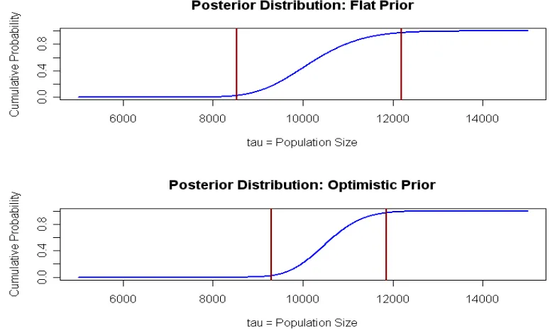
If we cut off 2.5% of the probability from each end of the posterior distribution, then we get the 95% Bayesian probability interval (8530, 12,198) of length 3668, which for practical purposes is similar to the confidence interval we obtained using the traditional method. This is called a probability-symmetric interval. If we cut of 1.5% from the shorter lower tail of the posterior distribution and 3.5% from the longer upper tail, we get the shorter interval (8381, 12021) of length 3640. One might search for the shortest possible 95% interval, but for simplicity it is customary to use probability-symmetric intervals. The R code for finding the posterior distribution, its mode, its median, and the probability interval is shown below. The cumulative distribution function of the posterior distribution and the 95% Bayesian probability interval are shown in the top panel of Figure 8.

tau = 5000:15000

prior = rep(1/length(tau), times=length(tau)) # discrete uniform prior

cond.99 = dhyper(99, 1100, tau-1100, 900) denom = sum(prior*cond.99)

post = prior*cond.99/denom; cumpost = cumsum(post) max.post = tau[post==max(post)]; mean.post = sum(tau*post) lcl = min(tau[cumpost> .025])

ucl = max(tau[cumpost< .975])

For practical purposes, either of these Bayesian intervals is essentially the same as the interval (8392, 12,086) of length 3694 obtained by the general method in Section 4.1. It is typical of flat or

uninformative prior distributions that they give numerical results similar to those obtained by non-Bayesian or so-called frequentist methods. There are, however, some philosophical differences between the interpretations frequentists make of confidence intervals and those Bayesians make of probability intervals.

 Frequentists use the word confidence precisely to avoid using the word probability. Either the confidence interval covers the true fixed value of the parameter or it does not. There is no probability about it. The figure 95% refers to the possibility that the process giving rise to the interval might be repeated frequently and the belief that the process will give the right result 95% of the time.

 For Bayesians the prior distribution on the parameter establishes a probability reference from the start. A combination of the prior distribution and the data yields the posterior distribution, from which the 95% probability interval is then derived. Bayesians believe there is a 95% probability that the interval is a true statement about reality.

An important advantage of the Bayesian method is that it can take prior knowledge or expert opinion into account. This is done by selecting a prior distribution that reflects the information we want to take into account before the experiment is done.

For example, consider a negative binomial distribution of a random variable that counts the number of trials until the success number n = 150, where P(Success) = 0.01375. It has a roughly normal shape, mean = 150/0.01375 = 10,909, and 95\% of its probability between 9500 and 12,400. In terms of our goal of increasing the fish population of the lake, this corresponds to a prior view that is a little more “optimistic” than our experiment alone turns out to indicate.

Figure 8. Cumulative posterior distributions (blue curves) and 95% Bayesian probability intervals (red lines) based capture-recapture results with X = 99. The upper panel shows results from a flat prior and the lower panel shows the narrower interval from an optimistic informative prior.

Based on this optimistic prior distribution, the Bayesian probability interval estimate of is (9301, 11,853). The mode of the posterior distribution is 10,457 and its mean is 10,519(see the bottom panel of Figure 8). Taken together, the information in the experiment and the optimistic prior distribution yielded a slightly larger point estimate with a sharper (narrower) interval estimate than we obtained using the relatively uninformative flat prior distribution. (The length of the interval from the flat prior is 3668 fish compared with an interval of length 2552 from the optimistic prior.) The R code is the same as that in Section 6.2 except that we use prior=dnbinom (tau-150,150,.01375)to specify the prior distribution. (The reason for subtracting 150 is that the form of the negative binomial distribution programmed into R counts only the number of failures before the nth success instead of the total number of trials until the nth success is seen.)

Bayesian results are a melding of prior opinion with experimental results. If the prior distribution contains information that we consider to be of value, we will regard the Bayesian method as an improvement over ones that disregard the prior information.

knowledge. For example, in our capture-recapture example, at a minimum our design is based on the

assumption there are at least 1100 fish in the lake. By contrast, if we were expecting a million fish in the lake our design would surely have been different, because estimation is unsuccessful if we recapture no tagged fish.

Another factor that has delayed the widespread use of Bayesian methods in practical applications is that the computation of a posterior distribution from the prior distribution and the data can sometimes be analytically intractable and computationally intensive. Only recently has the computer power been available to handle a broad range of Bayesian methods.

Our application to a capture-recapture experiment has the advantage that the parameter takes discrete values, so that it is possible to use the version of Bayes’ Theorem found in almost all beginning probability books to find the posterior distributions.

7. Conclusion

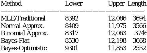
We have seen how a capture-recapture experiment can provide estimates of the size of a population. Table 3 summarizes some of the point and interval estimates we have obtained in this article.

Several Interval Estimates of Population Size .

Method Lower Upper Length —————————————————————— MLE/Traditional 8392 12,086 3694 Normal Approx. 8409 11,975 3566 Binomial Approx. 8317 12,063 3746 Bayes-Flat 8530 12,198 3668 Bayes-Optimistic 9301 11,853 2552

Table 3.Summaries of interval estimates for based on various methods.

Point estimates from the method of moments, the method of maximum likelihood and a Bayesian approach with an uninformative prior are similar.

If the informative prior information used in the Bayesian method is believed to be of value, then this method yields, by far, a tighter interval than the other methods illustrated here.

All of the computations and graphs in this article were done using R software, which is becoming an indispensable tool for statistical researchers and practitioners.

Current research on capture-recapture methods centers on weakening some of the very strong assumptions we have made here (for example, perfect mixing of the fish and no change in the population between capture and recapture) and on useful ways to exploit prior information.

7.1. Other Applications. Modern applications of capture-recapture methods go far beyond our simple

example of estimating the population size of fish in a lake. In this article we have used two samples (one at the capture phase and one at the recapture phase).

For example, a study by Hickman, Cox, et al.(1999) illustrates some generalizations of the basic capture-recapture experiment. Because it is notoriously difficult to obtain direct estimates of problem drug use just by taking a survey these investigators have used a scheme to obtain an indirect estimate of the prevalence of problem drug use in inner London that involves several samples from three different studies.

The goal of the Hickman study is to obtain evidence that can be used for effective policy making about interventions to help problem drug users. Information involves numbers of problem drug users in samples arising from a drug misuse database, from police and court contacts, and also from hospital records and HIV testing programs. Because problem drug use, as defined in the UK, encompasses both criminal and health problems it seems natural to seek data from sources related to both of these aspects. In each case, individuals who are problem drug users were identified as members of a larger population, and a universal ID system used in the UK makes it possible to identify “re-captures.” Because such samples from human populations are seldom independent, a major feature of the Hickman paper is to use the methodology of log linear models to assess and correct for association among the samples.

References

Brown, L. D.,Cai, T.T., and DasGupta, A. (2001),“Interval estimation for a binomial proportion,

“Statistical Science, 16:2, pp. 101–133.

Chao, A, (2001), “Estimation of Animal Abundance and Related Parameters,” Journal of Agricultural, Biological, and Environmental Statistics, Vol. 6, No. 2, pp. 158-175

Chao, A; Tsay, P. K., Lin, S. H., Shau, W. Y., and Chao, D. Y. (2001), "The applications of capture-recapture models to epidemiological data". Statistics in Medicine20 (20): 3123–3157

Chapman, D.G. (1951). Some properties of the hypergeometric distribution with applications to zoological sample censuses, Univeristy of California Press, Berkeley (book)

Feller, W. (1950), “An Introduction to Probability Theory and Its Applications,” Vol. I, 1st ed., Wiley, and Chapman & Hall

Feller, W. (1968), “An Introduction to Probability Theory and Its Applications,” Vol.I, 3rd ed., Wiley. Hickman, M.,Cox, S., Harvey, J, Howes, S., Farrell, M., Frischer, M., Stimson, G., Taylor, C. Tilling, K.,

(1999) “Estimating the prevalence of problem drug use in inner London: a discussion of three capture-recapture studies,” Addiction, Nov. 94(11), pp. 1653-62.

Lincoln, Frederick C. (May 1930). “Calculating Waterfowl Abundance on the Basis of Banding Returns,” Circular118. Washington, DC: United States Department of Agriculture. Retrieved 21 May 2013.

Petersen, C. G. J. (1896). "The Yearly Immigration of Young Plaice Into the Limfjord From the German Sea", Report of the Danish Biological Station (1895), 6, 5–84.