3 Iranian Journal of Chemical Engineering
Vol. 6, No. 3 (Summer), 2009, IAChE
Experimental and CFD Studies on the Effect of the Jet Position on
Mixing Performance
A. Parvareh1, M. Rahimi1∗ and Ammar Abdulaziz Alsairafi2
1- CFD Research Center, Chemical Engineering Department, Razi University, Kermanshah, Iran.
2- Faculty of Mechanical Engineering, College of Engineering and Petroleum, Kuwait University, Kuwait.
Abstract
The effect of jet positions on the homogenization progress of a dye in a rectangular tank equipped with a jet was studied. Water entered the tank laterally from the top and left the tank from the opposite wall at the same height. The suction position was fixed at one of the tank corners and seven positions were considered for the jet nozzle. A predefined volume of the dark Nigrosine was injected to the tank input as the tracer during 4s in all experiments. During the dye injection and mixing progress, the front and bottom views of the tank were recorded by a digital camera. The experimental results showed that as the jet nozzle was installed in the opposite wall from the tank input, the worst performance was obtained in comparison with the other jet positions. However, the jet nozzle position of 90° with respect to the tank input had the best performance. All of the experiments were modeled by Computational Fluid Dynamics (CFD). Finally, the CFD predicted dye spreading was verified by the experimental observations and a good agreement was observed between the CFD and experimental results.
Keywords: Jet, Homogenization, Mixing, CFD, Modeling
∗ Corresponding author: [email protected]
1- Introduction
Mixing has always had an important role in industrial processes and their operations and it is accomplished to achieve an homogenous solution. In chemical industries it can be used for homogenization of solutions and their properties, prevention of sedimentation, enhancing heat and mass transfer rates and chemical reactions. Mixing by impellers and jets are two known methods for fluid
4 Iranian Journal of Chemical Engineering, Vol. 6, No. 3 respectively relative velocity between the jet
and the tank fluid causes the forming of turbulent fluid layers in the boundaries of the jet. So the rotation of the fluid in the tank and the connecting pipes between the pump and tank mixes and homogenizes the tank solution.
One of the earliest studies about jet mixing was done by Fosset et. al [1]. They worked on mixing of large fuel tanks with a diameter of 40m by jets with different angles. Fox and Gex [2] continued their studies on both laminar and turbulent stream regimes and compared the effectiveness of jet mixing and mixing by impellers. Lane and Rice [3] showed that the mixing time at various Reynolds numbers has two different trends in laminar and turbulent regimes.
Maruyama et. al [4] worked on computing mixing times in cylindrical tanks and found that it is dependent on fluid depth, nozzle height and nozzle angle. Unger et al. [5] characterized laminar viscous flow in an impinging jet contactor using CFD and Particle Image Velocimetry (PIV) measure-ments. They found that mixing time can be improved substantially in the a symmetrical geometry. In continuation of this study, Unger and Muzzio [6] used the Laser-Induced Fluorescence (LIF) technique in order to quantitatively compare the mixing performance between two impinging jet geometries. Brooker [7] studied the performance of jet mixing using CFD. In his study, the mixing time with a maximum error of 15% was reported. The flow pattern and mixing time in a jet mixed tank equipped with various types of jets were predicted by Ranade [8]. He used the standard k−ε model in his CFD modeling. A non
convincing validation of the predicted results with the experiment was reported. Jayanti [9] studied the hydro-dynamics of jet mixing using various jet configurations in a cylindrical vessel. He focused on finding a way to reduce the mixing time by eliminating the dead zones in the vessel.
Patwardhan [10] compared the CFD prediction and the experimental mixing results of sodium chloride solution in a 98 liter tank. Hjertager et al. [11] used the CFD method to model a fast acid–base neutralization reaction in a tubular reactor. A modified Eddy Dissipation Concept (EDC) model was found to be suitable for simulating liquid phase reactions. After comparing the model predictions with experimental data, they concluded that although such an approach is efficient and useful in understanding reacting flow behavior, it might be inadequate to describe reactors involving complex reactions.
Iranian Journal of Chemical Engineering, Vol. 6, No. 3 5 They concluded that when the angle between
the jet and the impeller are 15° and 60°, the homogenization time is lower than that of other layouts.
In the present study, the effect of jet position on the mixing progress for a rectangular pilot scale tank has been investigated experi-mentally and theoretically. This work is done in a pilot plant scale based on an industrial scale reactive mixing case in the final pH correction pit of the Bistoun Pilot Plant, Iran. In this tank the reutilization reaction should take place on a waste water stream.
2- Experiments
The experiments were carried out in a cubic vessel with a volume of 125 liters filled with water. The tank inlet and outlet diameters were the same and equal to 4 cm. The feed was fed into the tank from a large reservoir in a way that the tank inlet linear velocity was fixed at 0.045 m/s. No wall was used for the top side of the tank and the fluid top level was in contact with the atmospheric air. The nozzle and suction diameters were 6 and 8 mm respectively. The fluid in the tank was withdrawn via a pump from the suction and was returned to the tank through the nozzle. A constant jet velocity of 4.35 m/s was set in all experiments. In this velocity the flow regime is turbulent as the Reynolds number is almost 35000.The jet Reynolds number has been defined based on the jet output linear velocity (U), the nozzle diameter (D) and kinematics viscosity (v) of working fluid as follows:
ν
UD
=
Re (1)
A constant position for the suction and seven
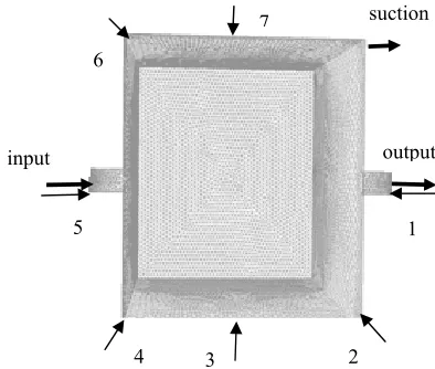
different jet positions were used to investigate the effect of jet position on the homogenization progress in the tank. Fig. 1 shows the position of the suction and seven positions of the nozzle.
Figure 1. A scheme view of the experimental tank with the nozzle and suction positions
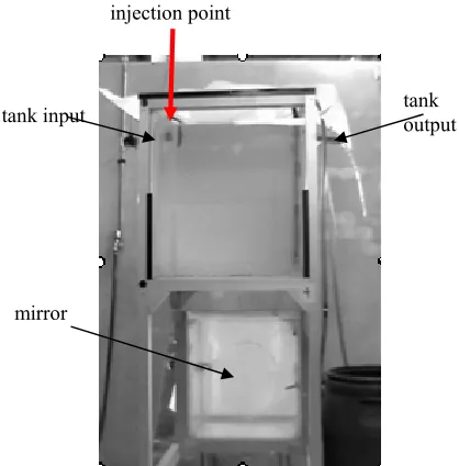
In all cases the nozzle and suction were set at a constant height of 5 cm from the tank bottom and the jet angle was fixed at 22.5º with respect to horizon. In all of the experiments, after the flow stabilization in the tank, 80 ml of the dark Nigrosine solution was injected close to the inlet stream during 4s .The tracer movement inside the tank was recorded by a digital camera from the front and bottom views. For this purpose, a mirror was fixed at a 45° angle with respect to the horizontal line under the tank. Three light sources were used around the tank to improve the recorded film quality. Fig. 2 shows the pilot tank and its detail.
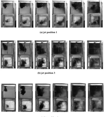
In order to investigate the homogenization trend and the quality of mixing in the tank, those captured at various time steps have been compared. As an example, Fig.3 shows the front and bottom views of the tracer movement in the tank for jet positions of 1, 3
7 suction
output input
6
5
4 3 2
6 Iranian Journal of Chemical Engineering, Vol. 6, No. 3 and 4 as the worst, best and intermediate
homogenization performances, respectively.
Figure 2. The pilot tank and its details In all cases, the tracer was injected close to the tank surface. As can be seen in this figure, due to the flow pattern established in the tank, the tracer movement differs for different positions of the jet. For example, in the first position, the dye prefers to withdraw from the tank directly and exit the tank before reaching a suitable homogenization. Therefore, position 1 causes the worst homogenization performance in comparison with the other investigated positions. However, in the other jet positions, the tracer penetrates more into the lower layer and mixes with the circulating fluid, leading to a better homogenization performance. According to the mixing progress shown in Fig.3, jet position 3 is the best location for tracer dispersion. In this case, the dye moves downward and mixes with water and goes toward the tank bottom. Consequently, it is dispersed by the jet outlet stream and is pushed toward the top. This causes
homogenization to take place in a more efficient way in position 3 in comparison with the other positions. Mixing by a jet placed in Position 4 was presented as an example of intermediate performance. In this position the jet was placed diagonally. After the tracer injection, it prefers to move toward the bottom layers. However, in contrast with position 3, in this position the tracer does not move toward the bottom right corner because of the jet position. Therefore, the homogenization can not occur appropriately in this position. However, the mixing progress in this position is better than position 1.
3- Theory
The CFD modeling involves the numerical solution of the conservation equations in the laminar and turbulent fluid flow regimes. Therefore, the theoretical predictions are obtained by simultaneous solution of the continuity and the Reynolds-Averaged Navier-Stokes (RANS) equations.
The crucial difference between the modeling of laminar and turbulent flows is the appearance of eddying motions of a wide range of length scales in the turbulent flows. The random nature of a turbulent flow precludes computations based on a complete description of the motion of all the fluid particles. In general, it is most attractive to characterize the turbulent flow by the mean values of flow properties and the statistical properties of their fluctuations. Introducing the time-averaged properties for the flow (mean velocities, mean pressures and mean stresses) to the time dependent Navier-Stokes equations, leads to time-averaged Navier-Stokes equations as follows [15]:
tank input
mirror
Iranian Journal of Chemical Engineering, Vol. 6, No. 3 7
Figure 3. Tracer dispersion for three jet positions
Continuity equation:
( )
+∇⋅( )
=0∂ ∂
V
t ρ ρ (2)
Momentum equation:
( )
V(
VV)
(
(
)
V)
Ft +∇⋅ =∇⋅ + t ∇ +
∂
∂ ρ ρ μ μ (3)
Where V is the velocity vector, μt is the turbulent viscosity, obtained from a turbulence model. The F parameter contains those parts of the stress term not shown explicitly as well as other momentum sources, such as drag from the dispersed phase. In addition, a species transport equation should be used for tracking the tracer in the present study[15].
(a) jet position 1
(b) jet position 3
8 Iranian Journal of Chemical Engineering, Vol. 6, No. 3 Based on previous experience [13], the RNG
[16] version of the k−ε model was employed as the turbulence model. In this model, the effect of small-scale turbulence is represented by means of a random forcing function in the Navier-Stokes equations. The RNG procedure systematically removes the small scales of motion from the governing equations by expressing their effects in terms of larger-scale motion and a modified viscosity. The f standard coefficients of this model were used in the modeling [16]. For the liquid and gas contact at the mixing tank surface, the Volume of Fluid (VOF) model was employed. Using this model, the interface between two phases (water and air) remains fixed [17]. Numerical stability is generally easily obtained because the flow field calculations are not coupled with identification of the free surface location [15].
4- CFD Modeling
As shown in the experiments, the worst and the best mixing performances were obtained when jet positions 1 and 3 were chosen, respectively. In the modeling part, these two positions were modeled and the CFD
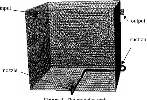
predictions for mixing progress were compared with the experimental results. In the present work, the pilot tank with a dimension of 0.5×0.5×0.5 m3 was modeled using the commercial CFD package, FLUENT6.2. The modeling domain was divided into 687342 and 713170 unstructured tetrahedral meshes according to the nozzle position for first and third jet positions respectively. These mesh layouts were found by examination of different cell sizes as no further significant change was obtained for finer cells. Fine meshes were used for sensitive regions such as nozzle and suction regions in order to increase the prediction precision. Fig.4 shows a view for the meshed tank and its detail.
The boundary conditions of the model were exactly set similar to the experimental ones. In the VOF modeling of free surface, the applied pressure on the surface of the tank was set at 101.325Kpa. The SIMPLE pressure-velocity coupling, the standard pressure, the first order upwind discretization scheme for momentum, turbulent kinetic energy and dissipation energy were employed in the modeling. The applied convergence criterion was selected to be 10-7.
Figure 4. The modeled tank nozzle
input
output
Iranian Journal of Chemical Engineering, Vol. 6, No. 3 9 In the modeling, the appropriate constant
linear velocity was defined for jet outlet and suction inlet streams. On the other hand, a constant linear velocity was introduced for the tank inlet stream, while for the tank output stream the "outflow" boundary condition was defined. The top layer of the fluid in the tank, which is in contact with atmospheric air, was defined as a free surface. So, the pressure inlet has been chosen as the boundary condition for this region.
In the first step, the steady state calculations were carried out to find the established flow pattern in the tank. In the second step, unsteady state calculations with a time step of 0.01s were done after achieving a steady flow pattern to model the injected tracer dispersion.
5- Results and discussion
The velocity vectors of the fluid in a vertical slice that goes through the input/output channels are shown in Fig.5. The jet nozzle has an angle of 22.5° with respect to the horizon. As shown in Fig.5(a), for position 1, as the inlet flow goes toward the tank bottom, it hits the jet output flow at the tank top layers. This causes the flow to be diverted toward the tank outlet. In this case, the injected tracer cannot move toward the middle and bottom layers of the tank and the tracer is withdrawn toward the output. Therefore, this jet position causes poor mixing performance and the tracer exits from the tank without suitable dispersion. However, at position 3 where the nozzle has the 90° angle with respect to the tank inlet, the outlet jet hits the opposite wall near the fluid free surface and is divided into two
parts. The first one, which is the strong portion, circulates inside the tank and consequently moves toward the nozzle along the bottom wall. Another stream goes to the fluid surface and then circulates toward the tank center. Therefore, as shown in Fig.5 (b), the inlet stream goes toward the tank middle region and hits the bottom wall. Furthermore, the fluid flow moves the tracer toward the bottom and the tracer can mix with the fluid in a more efficient way. In this case, the tracer cannot move directly toward the output, which causes a more efficient mixing performance in comparison with the other one.
10 Iranian Journal of Chemical Engineering, Vol. 6, No. 3 tank was twice as much as other regions.
This confirms that the position 3 setup worked more efficiently in comparison with position 1. In addition, comparison between the experimental and CFD data in all regions
of the two positions shows a minor difference between the CFD calculations and the experimental data. As can be calculated from the table, the maximum error is less than 15% for all of the comparisons.
Figure 5. Velocity vectors at two vertical slices
Table 1. The percent of the colored area at different regions of the tank for the experimental test and CFD calculations.
position 1 position 3
time(s) top middle bottom top middle bottom
Exp. CFD Exp. CFD Exp. CFD Exp. CFD Exp. CFD Exp. CFD
3 89 90 9 8 2 2 60 63 33 30 7 7 21 85 84 11 12 4 4 27 31 44 41 29 28 33 45 46 42 41 12 13 15 17 42 39 43 44 40 49 45 41 43 10 12 28 26 33 31 39 43 44 33 37 42 40 25 23 32 30 32 33 36 37 47 24 26 49 46 27 28 33 34 33 33 34 33
(a) jet position 1 (b) jet position 3
Iranian Journal of Chemical Engineering, Vol. 6, No. 3 11
6- Conclusions
This study was performed in a pilot scale rectangular continuous flow stirred tank and the effect of jet position on the homogenization progress was investigated experimentally and theoretically. This study is a preliminary study of mixing with reaction in an industrial scale tank with a similar geometry. In the experimental part, it has been concluded that the position of the jet nozzle can be quite effective on mixing performance. The CFD modeling results illustrate that the way that the fluid is circulated by the jet and the relative position of the tank's inlet stream to the tank and the jet position is quite important in order to reach a more efficient homogenization. Among the studied jet positions, the worst and the best performance were obtained for position 1(180° with tank's inlet) and 3(90° with tank's inlet), respectively. In addition, the modeling results show a good agreement with the experimental results. Therefore, it can be concluded that the CFD can be used as a good theoretical tool for studying mixing in continuous flow stirred tanks equipped with a jet.
Acknowledgement
The authors wish to express their thanks to the Iranian West Regional Electricity Company for the financial support of this work.
References
1- Fossett, H., “The action of free jets in mixing of fluids”, Trans. Inst. Chem. Eng., 29, 322 (1951).
2- Fox, E.A., and Gex, V.E., “Single-Phase blending of liquids”, AIChE J., 2, 539 (1956).
3- Lane, A.C.G., and Rice, P., “An investigation of liquid jet mixing employing an inclined side entry jet”, Trans. Inst. Chem. Eng., 60, 171 (1982).
4- Maruyama, T., Ban, Y., and Mizushina, T., “Jet mixing of fluids in tanks”, J. Chem. Eng. Jpn., 15, 342 (1982).
5- Unger, D.R., Muzzio, F.J., and Brodkey, R.S., “Experimental and numerical characterization of viscous flow and mixing in an impinging jet contactor”, Can. J. Chem. Eng., 76, 536 (1998).
6- Unger, D.R., and Muzzio, F.J., “Laser-induced fluorescence technique for the quantification of mixing in impinging jets”, AIChE J., 45, 2477 (1999).
7- Brooker, L., “Mixing with the jet set”, Chem. Eng. J., 30, 16 (1993).
8- Ranade, V.V., “Towards better mixing protocols by designing spatially periodic flows-The case of a jet mixer”, Chem. Eng. Sci., 51, 2637 (1996).
9- Jayanti, S., “Hydrodynamics of jet mixing in vessels”, Chem. Eng. Sci., 56, 193 (2001). 10- Patwardhan, A.W., “CFD modeling of jet
mixed tanks”, Chem. Eng. Sci., 57, 1307 (2002).
11- Hjertager, L.K., and T.Solberg, B.H., “CFD modeling of fast chemical reactions in turbulent liquid flows”, Comp. Chem. Eng., 26, 507 (2002).
12- Zughbi, H.D., and Rakib, M.A., “Mixing in a fluid jet agitated tank: effects of jet angle and elevation and number of jets”, Chem. Eng. Sci., 59, 829 (2004).
13- Rahimi, M., and Parvareh, A., “Experimental and CFD investigation on mixing by a jet in a semi-industrial stirred tank”, Chem. Eng. J., 115, 85 (2005).
12 Iranian Journal of Chemical Engineering, Vol. 6, No. 3 15- Fluent user’s guide, Version 6.2, Fluent Inc,
Lebanon, NH (2005).
16- Yakhot, V., and Orszag, S. A., “Renormaliz-ation group analysis of turbulence.I. Basic theory”, J. Sci. Compu.t, 1, 1 (1986).
17- Hirt, C.W., and Nichols, B.D., “Volume of fluid (VOF) method for the dynamics of free boundaries”, J. Comput. Phys., 39, 201 (1981).
18- Matthews, B.W., Fletcher, C.A.J., and Partridge, A.C., “Computational simulation of fluid and dilute particulate flows on spiral concentrators”, Appl. Math. Model., 22, 965 (1998).
19- Esparza, C. E., Guerrero-Mata, M. P. and Rios-Mercado, R. Z. “Optimal design of gating systems by gradient search methods”, Comput. Mater. Sci., 36, 457 (2006).