A Gumbel Distribution Model to Describe Correlation Values in Random Latin Hypercube Experimental Designs for Model and Simulation Based Systems Engineering

ISSN: 2334-2986 (Print), 2334-2994 (Online) Copyright © The Author(s). All Rights Reserved. Published by American Research Institute for Policy Development DOI: 10.15640/jea.v4n2a1 URL: https://doi.org/10.15640/jea.v4n2a1

A Gumbel Distribution Model to Describe Correlation Values in Random Latin

Hypercube Experimental Designs for Model and Simulation Based Systems

Engineering

Alejandro S. Hernandez

1

Abstract

Experimentation is critical for trade-off analysis during design and development, as well as test phases of model based or model and simulation based systems engineering, or use of simulation based designs. Latin hypercube designs are effective experimental schemes that can save time and resources. However, they can also have highly correlated columns that present problems during post simulation analysis. Experimenters need a means to know if the Latin hypercube design that they plan to generate has a tolerable amount of correlation within its columns. A known probability model greatly aids this need. Application of the Kolmogorov-Smirnov goodness-of-fit tests shows the appropriateness of the Type 1 Gumbel distribution to model the smallest maximum absolute pair wise correlation from a set of random Latin hypercube experimental designs with equal dimensions (design points and factors). We estimate the Gumbel’s location and dispersion parameters using only information from the design environment. Results of this paper improve the scientist’s ability to plan better experiments for the specific study condition.

Keywords: Design of Experiments; Latin Hypercube; Gumbel Minimum; Kolmogorov-Smirnov.

1. Introduction

Latin hyper cubes are widely used for high-dimensional computer experiments (Kleijnen 2008, Buyske and Trout 2001). As Gianni, D’Ambrogio, and Tolk (2015) indicate, practitioners of model-based systems engineering (MBSE) and model and simulation based systems engineering (MSBSE) are particularly interested in efficient, general-purpose designs for examining systems with a large number of factors corresponding to unknown response surfaces. Yet, the inherently high correlations that can exist in these designs make the ensuing analyses problematic.

Efforts to reduce or eliminate correlations are often difficult, computationally expensive, and time consuming (Hernandez 2008, Cioppa 2002). Hernandez, Lucas, and Sanchez (2012) offer an alternative approach to reduce correlation via random Latin hypercube (RLH) generation. The results include a general expression (Equation 1) and policies for selecting appropriate design dimensions (design points – n and factors – k) to produce an RLH with an acceptable degree of correlation. A separate equation corresponds for each specific G (the number of RLHs with the same dimension from which to choose). However, G is not in the overall equation, thus limiting its utility. A defined probability model incorporating the variables n, k, and G becomes a powerful tool for planning better experiments.

 

2/3 1/3 2/3 1 1

/

0 2

3 3

ˆ ˆ ˆ ˆ

        

E min max

G

n k n k

, G = {10, 25, 50, 75, 100, 125, 150, 175, 200} (1)

Shaping the design environment—D Env(n, k, G)—tofind an acceptable RLH requires a quantum measure. Equation 2 computes correlation between any two column vectors,

X

iand

X

j, for a given design X, where

x

i is the mean value of column i.

1

2 2

1 1

[( )( )]

( ) ( )

n

i i j j

b b

b ij

n n

i i j j

b b

b b

X x X x

X x X x

 

 

 



 







, (2)

Since the major concern is with the magnitude of the correlation and not its direction, we focus on the

largest

2

k

 

 

 

_{absolute pair wise correlation values for a design with k factors. The maximum absolute value of pair}

wise correlations for any RLH is:map max |



ij |, ( i j)



_.

Consider any G number of RLHs with the same design dimensions (n, k). Each RLH has a specificmap

, resulting in





map

 

1, map



2, ...,



map G





_{.The ordered set contains a} map _{that is less than all other values,}





₍₁₎





_{( 2 )}





_{( )}

s.t. _map  _map ... _map

G _{. We designate}





min

(1)

_map  _map

as our primary measure, and its corresponding RLH as the best from G designs.

2. Data Farming RLH Designs—Analysis and Model Development

2.1. Generating RLH Data

Latin hypercube sampling treats input variables as random, but with known distribution functions. For each factor, j, is a related column in the design,

X

j, j = 1, …, k, where its value distribution is divided into “n strata of equal marginal probability 1/n.” Constructing the Latin hypercube is a matter of sampling each stratum once (McKay, Beckman, and Conover 1979). Patterson (1954) simplifies the process by using the median in each stratum to create a lattice of n design points; RLH generation basically corresponds to k independent permutations of the first n natural numbers. Producing hundreds of millions of RLHs becomes routine (Hernandez 2008).

This study required creating over 200,000,000 RLHs to analyze their min

map



values for comparison with the Gumbel distribution. We identify 115 design dimensions (n and k, n>k) using dimensional conventions from Cioppa (2002) and combine them with nine G values (10 to 200) from Hernandez, et al. (2012), for a total of1035DEnvs. For any specified DEnv there are 1000 observations from which to develop statistics, such as the average value of

min min



_map





_map

. Table 1shows

min

map



for G = 200, i.e. for D Env (65, 7, 200),

min

0.1483



_map 

Table 1: DEnv (n, k, G = 200). Valid design dimensions are combinations of n, k;n>k.

2.2. A Case for the Gumbel (minimum or min) Distribution

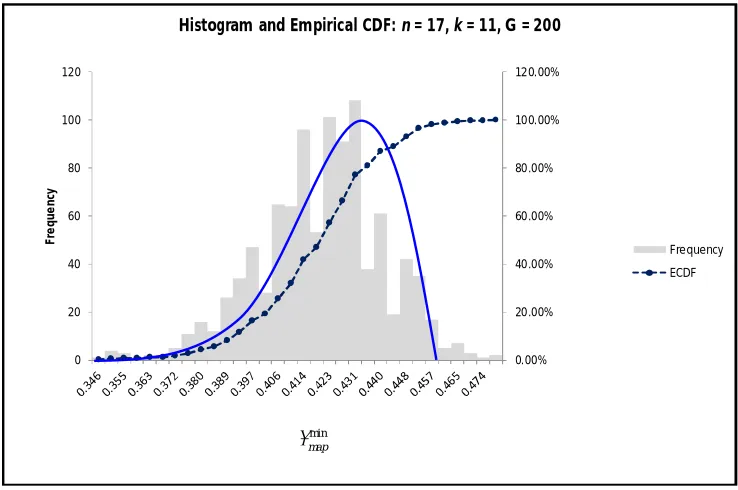
First level analysis of any DEnv is revealing. For instance, the frequency histogram Figure 1 shows 1000

min

map



values generated from DEnv (17, 11,200) as a negatively skewed bell curve, which indicates a Gumbel (min) distribution (1958). Kotz and Nadarajah’s (2005) validate the empirical CDF (ECDF) in Figure 1 for this Type 1 Gumbel distribution.

Figure 1: Frequency histogram of

min

map 

for DEnv(n = 17, k = 11, G = 200) shows a negatively skewed curve

indicative of the Gumbel (min) distribution; also known as the log-Weibull.

17 25 33 49 65 97 129 193 257 513 1025

7 0.3083 0.2463 0.2099 0.1727 0.1483 0.1214 0.1044 0.0851 0.0745 0.0521 0.0366

11 0.4163 0.3427 0.2936 0.2391 0.2065 0.1685 0.1468 0.1192 0.1035 0.0724 0.0511

16 0.4943 0.4027 0.3503 0.2864 0.2480 0.2029 0.1768 0.1436 0.1243 0.0875 0.0622

22 0.4508 0.3937 0.3216 0.2804 0.2299 0.1980 0.1612 0.1400 0.0991 0.0703

29 0.4271 0.3495 0.3041 0.2484 0.2159 0.1771 0.1529 0.1086 0.0768

37 0.3739 0.3264 0.2662 0.2309 0.1893 0.1630 0.1160 0.0821

46 0.3940 0.3417 0.2803 0.2438 0.1994 0.1726 0.1221 0.0866

56 0.3565 0.2927 0.2544 0.2083 0.1802 0.1279 0.0906

67 0.3037 0.2636 0.2158 0.1869 0.1329 0.0940

79 0.3129 0.2722 0.2232 0.1936 0.1371 0.0972

92 0.3220 0.2800 0.2295 0.1987 0.1409 0.0998

106 0.2862 0.2352 0.2037 0.1446 0.1024

121 0.2931 0.2399 0.2085 0.1477 0.1045

137 0.2448 0.2121 0.1505 0.1071

154 0.2493 0.2167 0.1532 0.1087

172 0.2533 0.2202 0.1561 0.1106

Mean Best of 200 RLH

n = Design Points

k =

Factors

0.00% 20.00% 40.00% 60.00% 80.00% 100.00% 120.00%

0 20 40 60 80 100 120

Fr

e

q

u

e

n

cy

Bin

Histogram and Empirical CDF: n = 17, k = 11, G = 200

Frequency ECDF

min map

The Gumbel (min) distribution has two parameters, α (location) and β (dispersion). Its probability density and cumulative distribution function (CDF) are in Equations 4 and 5, respectively(Gumbel 1958).For our case, the value, x, is the

min

map



.

1

( ) exp  exp  - ; > 0

  

 







_





_



_



_

   









x x

f x x

(4)

( ) 1 exp exp x - ; > 0

F x  x 





 



_





_



_



_

   









₍₅₎

Al-Subh (2014) effectively applies the method of moments to estimate β (Equation 6) and α (Equation 7) from sample data when the number of observations is 1000 or less:

6 ˆ

 

 

A s

, where s is the sample standard deviation, and (6)

ˆ ˆ

ˆ

_A    _{A, where}ˆ

is the sample mean and is Euler’s constant, 0.577216.(7)

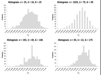
While we adopt the structure of Al-Subh’s formulas for parameter estimates, we recognize that they are directly dependent on empirical data. A method for estimating the Gumbel (min) parameters with only DEnv variables (n, k, G) is a much more useful and valuable prospect. The possibility to do so materializes from other DEnv graphs (Figure 2). They are similar to Figure 1, differing only in centrality and spread as n, k, and G vary.

Figure 2: Frequency histograms of 1000 observations of

min

map 

for different DEnv(n, k, G) show a change in

location and dispersion parameters.

0 10 20 30 40 50 60 70 80 90 100

Fr

e

qu

e

n

cy

Histogram: n = 25, k = 16, G = 25

min

map 

0 20 40 60 80 100 120 140 160 180

Fr

e

q

u

e

n

cy

Histogram: n = 193, k = 49, G = 100

min

map 

0 20 40 60 80 100 120 140

Fr

e

q

u

e

n

cy

Histogram: n = 65, k = 22, G = 175

min

map 

0 20 40 60 80 100 120 140 160 180 200

Fr

e

qu

e

n

cy

Histogram: n = 1025, k = 79, G = 50

min

2.3. DEnv Based Estimate for the Dispersion Parameter

Equation 6 depends on the sample deviation. We develop an expression for sample deviation in terms of DEnv(n, k, G) to estimate the dispersion parameters. The subscript H differentiates it from Al-Subh.

6

ˆ _ˆ

 

 

H s

, where sˆ is the DEnv based estimate for the sample standard deviation.(8) Generating and examining millions of

min

map



we formulate a regression model forsˆ. Logarithmic (Log) transformations of dependent and independent variables confirm a linear relationship between Log (Stdev) and Log of k:n ratios for different G values. Log (n) and Log(k) are similarly related to Log (Stdev).Equation 9 estimates the Log (Stdev) for a sample of

min

map



values. Computing

s

ˆ 10



Log Stdev( )completes Equation 8.

0 1 2 3 4 5 6

7 8 9

( ) ( ) ( ) ( )

( ) ( ) ( ) ( ) ( )

Log Stdev b b n b k b G b Log n b Log k b Log G

b kLog n b Log n Log k b Log k Log G

       

 

(9)

2.4. DEnv Based Estimate for the Location Parameter

To develop an appropriate estimate for α, we combine work from Al-Subh (2014) with that of Hernandez, et al. (2012). Al-Subh’s location parameter estimate relies on the sample mean, ˆ. We set

min

ˆ _map

 



and develop a new expression to estimate

min

map



that contains G.

Power transformations result in a strong linear relationship between transformed nand

min

map



.Equation 10is the new regression model for

min

map



, denotedas





m in E

m ap 

.



min



1/2 1/4 1/4 1/2 1/4 1/2 1/4 1/4

0 1 2 3 4 5 6 7

E

map b b n b k b n b k b G b n k b n k G

 _{   }  _  _  _   _   

(10)

Replacingˆwith





m in E

m ap 

in Equation 7 results in Equation 11, the DEnv based estimate for the location parameter. With ˆH_{, Equation 11 fully describes the DEnv based Gumbel (min).}



min



_ˆ

ˆ















E a

H m p H

(11)

3. Goodness-of-Fit Test for the Gumbel (min) Distribution

We test the goodness of the Gumbel (min) to model the min

map



K-S tests the null hypothesis H0:

F x

( )



F x

0

( )

against Ha:

F x

( )



F x

0

( )

, where

F x

0

( )

is the theoretical distribution. The estimate for

F x

( )

is

F x

ˆ( )

from observed data. We use Al-Subh’s (2014) parameter estimates to establish the theoretical distribution for the Gumbel (min) distribution and designate it as

F x

A

( )

_{. The test statistic} for the hypothesis test is the largest difference between CDF and ECDF:D=

ˆ

max ( ) A( )

x F x F x _{. If H}

0 is true, then

E F x





ˆ ( )

 



F x

A

( )

, thereby producing a small D. The value D is compared with a critical constant, C, corresponding to a specified confidence coefficient,  0.05 . The choice of Csatisfies



ˆ ( ) A( ) 0



P F x F x C H 



. Papoulis (1992) computes C based on choice of



: C =

1 ln

2m 2



    

 _{, where m}

is the number of observations. Failure to reject (FTR) the null hypothesis occurs if and only if D<C.

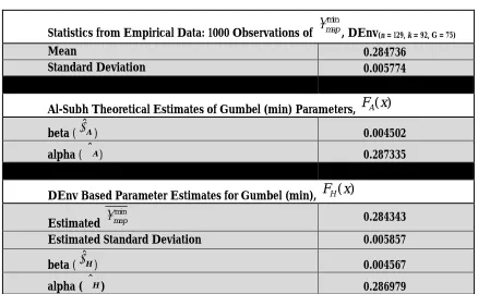
Table 2 summarizes statistics and parameter estimates for DEnv(n = 129, k = 92, G = 75) based on1000 observations of

min

map



. Comparisons of Al-Subh’s parameter estimates (2014) and the DEnv based Gumbel (min),

( )

H

F

x

, with statistics from the observed data demonstrate how consistent the DEnv based estimates are with the observed data, as well as Al-Subh’s parameters.

Table 2: Statistics from 1000 observations based on DEnv (129, 92, 75) and related estimates.

Statistics from Empirical Data: 1000 Observations of min

map



, DEnv(n = 129, k = 92, G = 75)

Mean 0.284736

Standard Deviation 0.005774

Al-Subh Theoretical Estimates of Gumbel (min) Parameters,

F x

A

( )

beta (ˆA_{) 0.004502}

alpha (ˆA_{) 0.287335}

DEnv Based Parameter Estimates for Gumbel (min),

F

H

( )

x

Estimated

min

map



0.284343

Estimated Standard Deviation 0.005857

beta (ˆH_{) 0.004567}

alpha (ˆH_{) 0.286979}

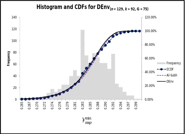
Figure 5: Comparison of ECDF with CDFs that result from Al-Subh and DEnv based parameter estimates. The data’s histogram shows the shape of the Gumbel (min).

K-S tests for all three distributions are equally convincing. Binned samples in Figure 5 include thirty-two separate points of comparison between the ECDF and CDFs. Table 3is an excerpt of these differences per binned,

xp. The greatest deviation occurs at xp= 0.28419, thus D= 0.06391.

Table 3: Test statistic for K-S test between ECDF and Al-Subh CDF, DEnv(n = 129, k = 92, G = 75).

xp 0.28081 0.28194 0.28306 0.28419 0.28532 0.28645 0.28758

ˆ( )

F x 0.22200 0.26200 0.38100 0.45600 0.51800 0.59700 0.66900

( )

A

F x 0.20907 0.26022 0.32113 0.39209 0.47249 0.56041 0.65222

ˆ ( ) ( )

  _A

D F x F x 0.01293 0.00178 0.05987 0.06391 0.04551 0.03659 0.01678

We compute the critical constant, C, that corresponds with the specified confidence coefficient,



, and number of observations, m = 1000. Based on the magnitude of the

min

map



values and observed standard deviations, we choose the confidence coefficient,  0.0001.The resultingCis0.07037; for any xp, a difference of more than 7%

between CDF and ECDF rejects the null hypothesis.

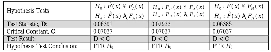
K-S tests for DEnv (129, 92, 75)are in Table 4. Column 2confirms that Al-Subh’s (2014) model for the Gumbel (min) distribution effectively describes the observed

min

map



values. The third column shows Al-Subh and the DEnv based Gumbel (min) are the same. Finally, column 4 verifies that there is no statistical difference between the DEnv based Gumbel (min) CDF and the ECDF. Columns 3 and 4 are the most critical for our purposes. With

( )

( )

H A

F

x



F x

, we further argue that

F

H

( )

x

_{is sufficient to describe the observed data.} 0.00% 20.00% 40.00% 60.00% 80.00% 100.00% 120.00%

0 20 40 60 80 100 120 140

0.

26

5

0.

26

7

0.

27

0

0.

27

2

0.

27

4

0.

27

6

0.

27

9

0.

28

1

0.

28

3

0.

28

5

0.

28

8

0.

29

0

0.

29

2

0.

29

4

0.

29

7

0.

29

9

Fr

e

q

u

e

n

cy

Bin

Histogram and CDFs for DEnv(n = 129, k = 92, G = 75)

Frequency ECDF Al-Subh DEnv

min

Table 4: Summary of K-S tests for DEnv(129, 92, 75).

Hypothesis Tests 0

ˆ

: ( ) ( )

ˆ

: ( ) ( )

A

a A

H F x F x

H F x F x

 

0 : ( ) ( )

: ( ) ( )

H A

a H A

H F x F x

H F x F x

 

0 : ˆ( ) ( )

ˆ

: ( ) ( )

H

a H

H F x F x

H F x F x

 

Test Statistic, D: 0.06391 0.02933 0.06385

Critical Constant, C: 0.07037 0.07037 0.07037

Test Result: D < C D < C D < C

Hypothesis Test Conclusion: FTR H0 FTR H0 FTR H0

4. Generalized Principles for Application

4.1. Policies for Using Gumbel (min) Models with DEnv Based Parameter Estimates

We prescribe the bounds for applying the DEnv(n, k, G) based Gumbel (min) model. Limit theory, past studies, and structure of the parameter estimates guide how to implement the model.

There is very little variation in min

map



values beyond a given value of n. Owen (1994) proves that any pair wise correlation,

ij



, for a Latin hypercube, specifically a lattice Latin hypercube, has variance of (n – 1)-1_{. As n} increases, variance in correlation values approach zero. Since regression assumes measurable variability in the chosen response variable, the regression model to estimate

min



_map

is not suitable when n is very large. Large values of n also have consequences for Al-Subh’s (2014) dispersion parameter estimate. As the standard deviation of

min

map



values approaches zero, the estimate for



also approaches zero and causes the Gumbel (min), as defined in Equations 4 and 5,to be undetermined. The ratio of k and n, which indicates the saturation of the design, affects the utility of a regression model. The term, (1 – k/n), appears in the denominator of the variance estimator for the regression model (Wu 1986). As the design reaches full saturation, i.e.,k/n = 1, the errors in the regression model greatly increases, thereby decreasing its usefulness.

Past studies inform the rule set in applying a DEnv based Gumbel (min) model for min

map



. Hernandez (2008) shows that RLHs with k/nless than 0.33 are more likely to have acceptable correlation values. Al-Subh (2014) uses values of n100in his effort to develop parameter estimates. Bolarinwa and Alhassan (2013) commonly work with values ofn = 20 or 100. Conditions for using a DEnv based Gumbel (min) distribution to model

min

map



values follow:

17n200_; 0.20 0.40

k n  

;

7



_

 

_{ }

( 10)



_

 100

 





k

n G

n

.

Within these bounds, the experimenter can select from a large number of DEnv combinations. We randomly draw twenty DEnvs that conform to the above criteria and apply K-S tests for null hypotheses:

0: ( )ˆ  A( ) H F x F x

, H0:F xH( )F xA( )_, H F x0: ( )ˆ F xH( )_{. The data comes from generating 1000 observations of}

min

map



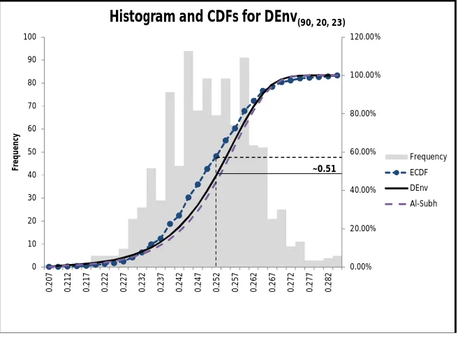
4.2. Applying DEnv Rules to the Experimental Condition

Consider an experimental condition to examine k = 20 factors. The analyst wishes to use an RLH design such that 0.25 and k/nless than 0.25, which leads to n = 80 design points and G = 23. Equations 8 through 11 determine the parameter estimates for the DEnv based Gumbel (min):

( )

ˆ 10Log Stdev = 0.01311

s _,





min 0.26291   E map , 6

ˆ _{ˆ 0.01023}

 

  

H s

, and

 

min

0.2688

= 1

ˆ ˆ =

  _H

E

map H

.

The experimenter computes the





min

0.25 0.133



 _map  P x

, a relatively low probability of creating the desired RLH. However, there is a greater than 80% chance of producing a RLH with correlation 0.275 or less under the same DEnv. If 0.275is unacceptable, the analyst can change any of the DEnv variables (experimental conditions). Increasing n to 90 improves the likelihood of creating an RLH with correlation 0.25 or less to51% (See Fig. 6), while increasing G to 30 betters the chances to 65%. Figure 6 illustrates the corresponding ECDF from 1000 RLH with design conditions n = 90, k = 20, G = 23, and presents Gumbel (min) CDFs for DEnv and Al-Subh estimates. Choosing DEnv (90, 20, 23), we generate an actual RLH design with0.25.

Figure 6: Histogram, ECDF, and CDF for DEnv(90, 20, 23)and Al-Subh

5. Conclusions

The Gumbel (min) distribution is an appropriate model to describe the

min



_map

values associated with RLH designs. Examining hundreds of millions of RLH and their

min



_map

values, we follow Al-Subh’s (2014) structure, but create parameter estimates for the Gumbel (min) using only the values n, k, G.K-S tests establish that the DEnv based Gumbel (min) accurately describes

min map



. min map  0.00% 20.00% 40.00% 60.00% 80.00% 100.00% 120.00% 0 10 20 30 40 50 60 70 80 90 100 0 .2 0 7 0 .2 1 2 0 .2 1 7 0 .2 2 2 0 .2 2 7 0 .2 3 2 0 .2 3 7 0 .2 4 2 0 .2 4 7 0 .2 5 2 0 .2 5 7 0 .2 6 2 0 .2 6 7 0 .2 7 2 0 .2 7 7 0 .2 8 2 Fr e q u e n cy

Histogram and CDFs for DEnv(90, 20, 23)

Frequency ECDF DEnv Al-Subh

The ability to equate a known probability distribution to model the behavior of correlation values in RLH experimental designs is an important tool for scientists applying MBSE, MSBSE, or simulation based designs. Understanding the situations in which DEnv based Gumbel (min) are applicable help experimenters choose the values of n, k, and G that will produce an RLH design that has correlation less than or equal to a specified

min

map



. The analyst can quickly determine the probability of generating a design with an acceptable degree of correlation from the DEnv condition before expending time and resources to develop the experimental plan.

Efficient experimental designs applied in MSBSE provide great incentives. Such experiments are critical for identifying significant factors in system design and trade-off analysis. With the same scheme, early simulation of systems can improve development of better stressor scenarios for test and evaluation through post-war-game experimentation and analysis (Hernandez, McDonald, and Ouellet 2015). The Gumbel (min) model in this paper is applicable as a simple routine for any software that generates Latin hypercubes. Accordingly, we offer it to experimenters and scientists.

6. References

Al-Subh, S.A. (2014). Goodness of Fit Test for Gumbel Distribution Based on Kullback-Leibler Information Using Several Different Estimators. Applied Mathematical Sciences, Vol. 8, No. 95, 4703 – 4712.

Bolarinwa, L.A. and Alhassan, B.G. (2013).An Investigation of the Performance of Kolmogorov-Smirnov and Anderson-Darling Goodness of Fit Statistics on Pareto and Gumbel Minimum Densities. International Journal of Advanced Scientific & Technical Research. Issue 3, Vol. 1.

Buyske,S. and Trout,R. (2001).Advanced Design of Experiments. Statistics 591 Lecture Series. Rutgers University. Cioppa, T.M. (2002).Efficient Nearly Orthogonal and Space-Filling Experimental Designs for High-Dimensional Complex

Models.Ph.D., diss. Naval Postgraduate School.

Gianni, D., D’Ambrogio, A., and Tolk, A. (2015).Model and Simulation-Based Engineering Handbook. Florida: Taylor and Francis Group, LLC, (Chapter 5).

Gumbel,E.J. (1958). Statistics of Extremes.USA: Echo Point Books & Media, LLC.

Hernandez, A.S. (2008). Breaking Barriers to Design Dimensions in Nearly Orthogonal Latin Hypercubes. Ph.D., diss. Naval Postgraduate School.

Hernandez, A.S., Lucas, T.W., and Sanchez, P.J. (2012).Selecting Random Latin Hypercubes Dimensions and Designs through Estimation of Maximum Absolute Pairwise Correlation. Proceedings of the 2012 Winter Simulation Conference.

Hernandez, A.S., McDonald, M.L., and Ouellet, J. (2015).Post Wargame Experimentation and Analysis: Re-Examining Executed Computer Assisted Wargames for New Insights. Military Operations Research Journal, Vol. 20, No.4, 19 – 37.

Kleijnen, J.P.C. (2008). Design and Analysis of Simulation Experiments. New York: Springer Science and Business Media, LLC.

Kotz,S. and Nadarajah, S. (2005).Extreme Value Distributions: Theory and Applications. London, UK: Imperial Press. Mckay, M.D., Beckman, R.J., and Conover, W.J. (1979).A Comparison of Three Methods for Selecting Values of

Input Variables in the Analysis of Output from a Computer Code. Technometrics. Vol. 21, No. 2, 239 – 245. Owen, A.B. (1994). Controlling Correlations in Latin Hypercube Samples. Journal of the American Statistical Association.

Vol. 89, No. 428, 1515 – 1522.

Papoulis, A. (1992). Probability & Statistics. Englewood Cliffs, NJ: Prentice Hall.

Patterson, H.D. (1954). The Errors of Lattice Sampling. Journal of the Royal Statistical Society, Series B (Methodological). Vol. 16, No. 1, 140-149.