Qubitization of Arbitrary Basis Quantum Chemistry Leveraging Sparsity and Low Rank Factorization

Qubitization of Arbitrary Basis Quantum Chemistry

Leveraging Sparsity and Low Rank Factorization

Dominic W. Berry

_{, Craig Gidney}

_{, Mario Motta}

_{, Jarrod R. McClean}

_{, and Ryan}

Bab-bush

1_{Department of Physics and Astronomy, Macquarie University, Sydney, NSW 2109, Australia} 2_{Google Research, Venice, CA 90291, United States}

3_{Division of Chemistry, California Institute of Technology, Pasadena, CA 91125, United States}

2019-11-27

Recent work has dramatically reduced the gate complexity required to quantum simulate chemistry by using linear combinations of unitaries based methods to exploit structure in the plane wave basis Coulomb operator. Here, we show that one can achieve similar scaling even for arbitrary basis sets (which can be hundreds of times more compact than plane waves) by using qubitized quantum walks in a fashion that takes advantage of structure in the Coulomb operator, either by directly exploiting sparseness, or via a low rank tensor factorization. We provide circuits for several variants of our algorithm (which all improve over the scaling of prior methods) including one withO(e N3/2λ)T complexity, whereNis number of orbitals andλis the 1-norm of the chemistry Hamiltonian. We deploy our algorithms to simulate the FeMoco molecule (relevant to Nitrogen fixation) and obtain circuits requiring about seven hundred times less surface code spacetime volume than prior quantum algorithms for this system, despite us using a larger and more accurate active space.

1

Introduction

Quantum computers were originally proposed as special purpose tools for efficiently modeling physical quantum mechanical systems [1]. Ever since then quantum simulation has been central to the study of quantum computing [2] while also regarded as one of its most promising applications. In recent years, progress in quantum hardware has led to great optimism for the field. However, a large gap remains between expectations for the technology and the expected value of the relatively few known applications that appear viable on even a small fault-tolerant quantum computer [3]. This disparity has underscored the importance of estimating and reducing the resources required to implement quantum algorithms within a fault-tolerant cost model.

The most widely studied and anticipated application of quantum simulation is chemistry [4]. Most work on this topic has focused on providing solutions to the electronic structure problem by using phase estimation to sample molecular eigenstates and estimate eigenvalues [5, 6]. Even at small problem sizes of around a hundred qubits, efficient and accurate solutions to this problem could prove transformative for various fields of study and the development of technologies such as better batteries, pharmaceuticals and industrial catalysts.

In order to represent molecular systems on a quantum computer one usually discretizes the many-body wavefunction using a basis of single-particle functions referred to as orbitals. The vast majority of quantum chemistry calculations use either plane wave orbitals, or more elaborate orbitals that are commonly composed of linear combinations of Gaussians. Plane waves are often chosen in calculations of periodic materials and lead to highly structured Hamiltonians. The work of [7] showed that exploiting this structure leads to asymptotic advantages for quantum

Dominic W. Berry:[email protected]

Ryan Babbush:[email protected]

algorithms. Today, the best-scaling quantum algorithms for chemistry in second quantization use plane waves; with eitherO(N3_{)gate complexity (with small constant factors) [8,9] orO(N}2_logN)

gate complexity (with large constant factors and more spatial complexity) [10].

A major limitation to using plane waves in second quantization is that one needs a very large number of spin-orbitals to represent many molecular systems to chemical accuracy. The work of [11] suggests resolving this problem by simulating the plane wave Hamiltonian in first quantization to achieveO(e N1/3η8/3)gate complexity, whereη is the number of electrons. With such low scaling inN, one might be able to use an extremely large plane wave basis. Unfortunately, the practicality of that algorithm is unclear because it has not been compiled to explicit circuits, and it is unclear how large the basis would need to be [10].

The more obvious remedy to the low resolution of plane waves is to use a more compact basis. Indeed, the majority of proposals for the quantum simulation of chemistry focus on using very compact molecular orbitals. However, using molecular orbitals leads to complex Hamiltonians with coefficients defined in terms of integrals andO(N4_{) distinct terms. As a consequence, the}

first quantum algorithms in this representation had gate complexityO(N11_{)[12,13]. Since then, a}

large community of researchers has worked to significantly reduce the cost of simulation in this rep-resentation through tighter bounds [13–15], better mappings between fermions and qubits [16–20], improved state preparation techniques [21–24], application of new time-evolution strategies [25–

27], considerations of fault-tolerant overheads [28–30] and other representational and algorithmic insights [31–36].

The lowest rigorous complexity of prior work on second quantized arbitrary basis chemistry simulation is either theO(e N5)scaling of [26], or theO(e λ2)scaling of [27], whereλis the 1-norm of the Hamiltonian. However, the [26] algorithm suffers from large constant factors in the scaling, and the approach of [27] scales quadratically worse than post-Trotter methods with respect to the evolution time. In practice, we expect the most competitive prior method would be Lie-Trotter product formulae [36], but the step size for that approach has not been studied. These results are challenging to compare directly because the scaling ofλwith respect toN depends on whetherN is growing towards the thermodynamic (large system) or continuum (large basis) limit. Here we provide an algorithm withO(e N3/2λ) T complexity, which appears better than all prior work so long asλ= Ω(N3/2_{), which is usually the case.}

Prior papers to compile a quantum chemistry algorithm to the level of Clifford + T gates and estimate the resources required within an error-correcting code are [8, 9, 29]. These papers focus on minimizing T complexity or Toffoli complexity because these gates cannot be transversely implemented within practical codes [30, 37]. To implement these gates one must distill magic states or Toffoli states, which takes orders of magnitude more spacetime volume (qubitseconds) than executing Clifford gates and also consumes a very large number of physical qubits [38,39].

The work of [29] focused on the simulation of an active space of the FeMo cofactor of the Nitrogenase enzyme, aka “FeMoco” (stoichiometryFe7MoS9C). FeMoco is the active site for the

catalytic conversion of Nitrogen gas into ammonia (fertilizer) in biological processes [40]. This reaction is of great importance; while the mechanism is not understood due to complex electronic structure, biological Nitrogen fixation is significantly more efficient than the industrial alternative. The paper by RWSWT [29] focused on a 108 qubit active space, and determined that roughly

1014 _{T gates would be required. If implemented in the surface code using gates with10}−3 _error

rates, the most efficient protocols for magic state distillation in this context require roughly 14 qubitseconds [30,37] of spacetime volume. At those rates, just distilling the magic states needed for [29] would require over four million qubitdecades (e.g., four million qubits running for a decade or a billion qubits running for two weeks), which is not practical.

The works of [8,9] show that one can perform similar sized chemistry simulations with roughly

108T gates, but in a plane wave rather than Gaussian basis. By application of techniques from [37] such calculations could be implemented in the surface code at10−3physical error rates with fewer than a million physical qubits in just hours. However, one would require far more plane waves to treat FeMoco, so these algorithms are not appropriate. In this paper, we develop an approach that has T counts somewhere in between those discussed in [8,9] and [29] and is compatible with compact molecular orbitals appropriate for a system like FeMoco.

query model [42]. Our analysis of the phase estimation algorithm is nearly identical to that in [8], which realizes a proposal suggested in [22,23] based on qubitization [25]. We make heavy use of the unary iteration technique introduced in [8] (see also a similar idea in [43]) as well as the QROM based state preparation and coherent alias sampling technique that was originally developed in [8] and then improved to lower T gate complexity in [44]. Finally, a key aspect of our algorithm is to leverage the sparse nature of the Coulomb operator, using a low rank representation recently discussed in [36].

In the case where we limit the number of ancilla qubits used, mostly using the system qubits as “dirty” ancilla, our algorithm can obtain chemical accuracy for FeMoco with about2×1013Toffoli gates, using the active spaces of either Reiher, Wiebe, Svore, Wecker, and Troyer (RWSWT) [29] or Li, Li, Dattani, Umrigar, and Chan (LLDUC) [45]. If we allow a large number of ancilla then the number of Toffoli gates achieved with our most efficient approach is about 2×1011 _{for the}

RWSWT orbitals, or8×1010 _{for the LLDUC orbitals. Throughout we focus on complexities in}

terms of Toffoli counts, because the non-Clifford gates we use are exclusively Toffolis. The cost in terms of T gates will be four times as large but since we are bottlenecked by Toffolis we can directly distill Toffoli states, which is possible with roughly the same cost as distilling two magic states for T gates [37]. Although we improve upon the distillation spacetime volume required by [29], at10−3 _{error rates we still require about three million qubitweeks of state distillation, which}

improves over previous results by roughly a factor of seven hundred, but is still substantial. The paper is organized as follows. In Section 2we review how it is possible to truncate the Coulomb operator to low rank, and establish notation. InSection 3we describe the Hamiltonian as a linear combination of unitaries, and how to perform the state preparation and controlled unitary operations. We give calculations of the complexities obtained with the low rank truncation for FeMoco inSection 4. InSection 5 andSection 6we discuss techniques that can be used to further lower the cost of qubitization based quantum chemistry simulations by leveraging unstructured sparsity that may exist in the Coulomb operator. We conclude in Section 7. In Appendix A,

Appendix B, and Appendix Cwe discuss technical details relating to how the qubitization state preparation oracle is implemented. InAppendix D we discuss the scaling of theλparameter for more general chemical systems. InAppendix Ewe give the details for minor contributions to the cost, and inAppendix Hwe give circuits and exact costings for arithmetic.

2

Low Rank Tensor Factorization of the Coulomb Operator

In this section we review representations of the Coulomb operator based on low rank tensor de-compositions. These ideas have existed in some form in the classical electronic structure literature for decades [46–51], and were recently discussed in the context of Trotter based electronic structure simulations in [36].

We first define the electronic structure Hamiltonian in an arbitrary second quantized basis as

H= X

σ∈{↑,↓}

N/2

X p,q=1

hpqa†p,σaq,σ+

1 2

X α,β∈{↑,↓}

N/2

X p,q,r,s=1

hpqrsa†p,αa

†

q,βar,βas,α (1)

= X

σ∈{↑,↓}

N/2

X p,q=1

Tpqa†p,σaq,σ+ X α,β∈{↑,↓}

N/2

X p,q,r,s=1

Vpqrsa†p,αaq,αa†r,βas,β (2)

where a†

p and ap are fermionic creation and annihilation operators for spin-orbital φp(r). The scalar coefficientshpq andhpqrsare the one- and two-electron integrals over the basis functions,

hpq= Z

dr1φ∗p(r1)

−∇

2

2 +U(r1)

φq(r1), (3)

hpqrs= Z

dr1dr2φ∗p(r1)φ∗q(r2)V(r1, r2)φr(r2)φs(r1), (4)

whereU(r1)andV(r1, r2)are the nuclear and electron-electron potentials, respectively. In Eq.(2)

Coulomb operator in so-called “chemist notation” witha†a a†ainstead ofa†a†a a, and absorbing the factor of 1/2 into the coefficients. Reordering operators according to the fermionic anticommutation relations{a†_p, aq}=δpqalso slightly changes the one-body coefficients.

Assuming real basis functions (such as molecular orbitals),TpqandVpqrsare real and have the symmetries [52],

Tpq=Tqp, Vpqrs=Vsrqp=Vpqsr=Vqprs=Vqpsr=Vrsqp=Vrspq=Vsrpq, (5)

which are important for properties of the tensor decompositions we will discuss. The rank-4 tensor V hasN/2 elements along each axis and we can reshapeV (e.g. using “numpy.reshape”) into an N2_/4×N2_{/4 matrixW which has composite indices pq (representing the first electron) and rs}

(representing the second electron). This procedure is commonly referred to in the applied math literature as the matricization of a tensor.

The W matrix is symmetric and positive semidefinite. It is important to emphasize here that we have focused on the spatial orbital representation of the two-electron integrals in the chemist ordering. In the physicist ordering, the resulting matrix has full rank, and no reduction of cost is possible. Similarly, introduction of fermionic symmetries induced in the full spin-orbital Hamiltonian into the coefficients (e.g. removing coefficients of terms likea†_ia†_jakak) will destroy the required structure for efficient simulation. This is because we are exploiting the low rank nature of the underlying spatial Coulomb interaction through matrix factorization, and it is easy to lose this structure if one is not careful. We will diagonalize it as

W g(`)=ω`g(`), W = L X `=1

ω`g(`)

g(`)

T

, (6)

where g(`) is the `th eigenvector ofW having size N2/4 and ω` ≥0 is its associated eigenvalue. Since we are takingV and henceW to be real, g(`)_{will also be real. The rank ofW is denotedL.}

If W were of full rank then it would be the case thatL =N2_{/4; however, the integrals that}

one encounters in molecular electronic structure applications contain considerable structure. As a consequence of this structure, it turns out thatW is not full rank, and insteadL ∈ O(N). The physical basis for this result is the pairwise nature of the Hamiltonian interactions, arising from the Coulomb kernel in a real-space representation. This property is regularly exploited in classical approaches to electronic structure in techniques such as “density fitting” [47,48] which is commonly performed using a Cholesky decomposition [49–51] (which is similar to the diagonalization in Eq.(6)

but is numerically more efficient and permits different left and right eigenvectors).

We use the notation gpq(`) to denote the entry of g(`) indexed by the composite index pq (the same composite index we used to flattenV intoW). The eigenvectorsg(`)inherit certain symmetry properties ofV, with the result thatgpq(`) is symmetric betweenpandq. We can express the two-electron operator in terms ofg(pq`)as

X α,β∈{↑,↓}

N/2

X p,q,r,s=1

Vpqrsa†p,αaq,αa†_r,βas,β = L X `=1

ω`  

X σ∈{↑,↓}

N/2

X p,q=1

g_pq(`)a†_p,σaq,σ  

2

. (7)

While common in electronic structure, this representation was first proposed in a quantum comput-ing context in [15]; however, that work did not appear to appreciate the low rank aspect, which was first exploited for advantage in quantum computing in [36]. Whereas there are O(N4)seemingly distinct coefficients on the left side of this equation, there areO(N2L) = O(N3) distinct coeffi-cients on the right side of the equation. Due to symmetry, the number of independent coefficoeffi-cients for each`isN2_{/8 +N/4, giving a total number ofL(N}2_{/8 +N/4).}

that second factorization in this work because it adds many intricacies, is less well understood than the first factorization, and might not offer an asymptotic advantage in T complexity for technical reasons related to the improved scaling that comes from using the improved “QROAM” discussed later in this work.

3

LCU based simulation

A number of techniques for simulating Hamiltonian evolution are based upon the linear combination of unitaries approach [42,54]. This approach enables one to achieve a sum of unitaries that yields another unitary operation. Say the operation to perform is given in the formU =P

jwjUj, where wj are real and positive. First a control register is prepared in the state Pj

p

wj/λ|ji, where λ=P

jwj is needed for normalization. We call this preparation operation “prepare”. Then a controlled Uj operation is performed on the target system, an operation we will call “select”. The inverse_prepareoperation is performed, then if the control system is measured in the state

|0i, then the operation U will have been applied to the target system. This operation only has probability1/λ2 _{of success, so to achieveU with unit success probability one can use∼λsteps of}

oblivious amplitude amplification.

This formalism was generalized by the block encoding, or “qubitization”, formalism of [25], where one can take the Hamiltonian to be a linear combination of unitaries, and use quantum signal processing [55] to obtain Hamiltonian evolution. For quantum chemistry, we are typically interested in the eigenvalues of the Hamiltonian. In that case, instead of performing the Hamil-tonian evolution, one can instead consider performing phase estimation on a single step from the qubitization formalism of [25]. This step corresponds to expressing the Hamiltonian as a linear combination of unitaries using twoprepare operations and one select operation, as well as a reflection as one would do for oblivious amplitude amplification. The eigenvalues of this step will then bee±iarccos(Ek/λ)_{, whereE}

k are the eigenvalues of the Hamiltonian. The complexity is fun-damentally dependent on the quantityλ=P

jwj. The overall complexity will be proportional to λmultiplied by the complexity of the_selectand_prepareoperations.

3.1

The Hamiltonian as a linear combination of unitaries

We can mapa†_paq+a†qap and the number operatornp=a†pap to qubits using the Jordan-Wigner transformation as

a†_p,σaq,σ+a†q,σap,σ7→

Xp,σZX~ q,σ+Yp,σZY~ q,σ

, a†_p,σap,σ7→

1

2(1−Zp,σ), (8)

whereX, Y andZ are the Pauli operators, the subscripts indicate the qubits these operators act on, andApZA~ q is shorthand forApZp+1· · ·Zq−1Aq. Thus, our Hamiltonian can be represented as

the linear combination of unitaries:

H 7→ 1 2

X p6=q,σ

Tpq

Xp,σZX~ q,σ+Yp,σZY~ q,σ

+1 2

X p,σ

Tpp(1−Zp,σ)

+1 4 X ` ω`   X p6=q,σ

g_pq(`)Xp,σZX~ q,σ+Yp,σZY~ q,σ

+X

p,σ

g(_pp`)(1−Zp,σ)  

2

. (9)

The terms in the first line in this expression correspond to the one-body operator T, and the terms in the second line correspond to the factorized two-body operator. Here the ranges of the summations are the same as forH.

Given the Hamiltonian expressed as a linear combination of unitaries, we can now give the expression forλ. In the following we will useλT to refer to the sum of weights for the one-body term as in Eq.(2), and useλW to refer to the sum of weights for Coulomb operator in its factorized form, as on the right-hand side of Eq.(7). We haveλ=λT +λW, with

λT = 2 N/2

X p,q=1

Here the factors of 2 and 4 in front of the sums are due to summation over the up and down spins. By simulating the factorized Hamiltonian we are slightly increasingλover what it would be if we used the Hamiltonian in its original form from Eq.(2). Denoting byλV the sum of weights for the potential term in the form Eq.(2), one has

λV = 4 N/2

X p,q,r,s=1

|Vpqrs|= 4 N/2 X p,q,r,s=1 L X `=1

ω`g(pq`)g

(`) rs ≤4 L X `=1 ω` N/2 X p,q,r,s=1 g (`) pq g (`) rs

=λW. (11)

However, we do not expect any difference between the asymptotic scaling of λV and λW with respect toN.

Because these quantities directly scale the complexity of our approach, techniques for reducing the effective value ofλare potentially important. Perhaps the simplest idea to reduceλmight be to optimize it under rotations of the single-particle basis (and to accordingly rotate the initial state using the Givens rotation technique in [56]). Another example of such a technique is to modify the Hamiltonian by adding to it a linear combination ofn-representability [57] equality constraints that have provably zero expectation value. This strategy was introduced and shown to be effective in Section V of [58]. Other techniques that might be useful for this include mean-field background subtraction [59] and the use of soft pseudopotentials [60]. However, one should make sure that these methods are applied in a way that does not increase the rank of the Coulomb operator, which would be counterproductive for the overall complexity. Note finally that interaction picture techniques [10] do not appear to be helpful here because whileλV λT, the V operator cannot be fast-forwarded.

In order to perform phase estimation via the qubitization/LCU approach, we need to be able to perform the state preparation prepare and controlled unitaries select. The techniques to achieve these operations are described in the following subsections.

3.2

State preparation

The state we would need to prepare is

|ψi=|0i |+i |0iX

p,q,σ r

|Tpq| λ |θ

(0)

pqi |0i |p, q, σi |0i

+X

` r

ω`

λ |`i |+i |+i X p,q,r,s,α,β

q

|gpq(`)g

(`)

rs| |θpq(`)i |θ

(`)

rsi |p, q, αi |r, s, βi, (12)

whereλis as defined in Eq.(10),|+i= (|0i+|1i)/√2,αandβ are spin labels, andθ(pq`)are used to obtain the correct signs on the terms. They are given by

θ_pq(0)=

(

0, Tpq>0,

1, Tpq<0,

θ(_pq`)=

(

0, g(pq`)>0,

1, g(pq`)<0.

(13)

The first register gives`, with|0i reserved for the first term. The first term gives the first two terms in Eq.(9), with the first term in Eq.(9) obtained forp6=qand the second term obtained forp=q. The|+istate on the second qubit selects between 1andZp,σ forp=q. We usep < q andp > q to select between Xp,σZX~ q,σ and Yp,σZY~ q,σ for p6=q, in a similar way as in [8]. The second term gives the third term in Eq.(9), with the sums over p, q andr, s yielding the square. The two|+istates in registers 2 and 3 select between 1 and Zp,α forp=q and between 1and Zr,β forr=s.

There are(L+ 1)(N2_{/8 +N/4) =O(N}3_{)unique coefficients, which indicates the state}

prepara-tion can be performed with similar complexity. Using the QROM and subsampling techniques from [8], the T complexity can be expected to be O(N3_{+ log(1/)), where is the required precision.}

By using a more sophisticated preparation scheme it will be possible to reduce the number of T gates, as will be described below.

1. Prepare a superposition over the first register, to produce the state  |0i v u u t X p,q

2|Tpq| λ + 2

X `

r ω`

λ |`i X

p,q

|g(_pq`)|



|0i |0i |0i |0i |0i |0i. (14)

2. Perform a Hadamard on the second register, and a Hadamard on the third register controlled on the state of the first register being|`ifor` >0, giving



|0i |+i |0i v u u t X p,q

2|Tpq| λ + 2

X `

r ω`

λ |`i |+i |+i X

p,q

|g(_pq`)|



|0i |0i |0i |0i. (15)

3. Prepare a superposition over register six controlled on the first register. For the first register in the state |0i, we prepare weights p|Tpq|, and for |`i with ` > 0 we prepare weights proportional to

q

|gpq(`)|. The state is then

|0i |+i |0iX

p,q,σ r

|Tpq|

λ |0i |0i |p, q, σi |0i

+√2X

` r

ω`

λ |`i |+i |+i X p,q,α

q

|gpq(`)| s

X r,s

|grs(`)| |0i |0i |p, q, αi |0i. (16)

4. Perform another state preparation on register seven, controlled on register one. For register

one in the state|`iwith` >0 we prepare weights proportional to q

|g(rs`)|, giving

|0i |+i |0iX

p,q,σ r

|Tpq|

λ |0i |0i |p, q, σi |0i

+X

` r

ω`

λ |`i |+i |+i X p,q,r,s,α,β

q

|g(pq`)grs(`)| |0i |0i |p, q, αi |r, s, βi. (17)

5. Use QROM to output|θ(pq`)iin register four and|θ

(`)

rsiin register five.

We will allow total error. Because there are a number of steps, each step will have an allowable error some fraction of . Here we aim to estimate the leading-order term in the complexity, and the allowable error will only appear in logarithms, so we will simply give log(1/), rather than subdividing the allowable error between the different steps. Throughout we will uselogto indicate logarithms to base 2.

For the state preparation in step 1, the approach in [8] gives complexity in terms of Toffolis L+O(log(1/)). The complexity in step 1 will be negligible compared to the complexity of later steps. The second step is just controlled operations on two qubits, and has negligible complexity compared to the other steps.

for each of theN/2 values of pthe complexity of iterating overq isN/2−1. That gives a total complexity for iterating overpandqthat isN2_/4−1.

As a result the complexity of the state preparation is N2_{/4 +O(log(1/)) for each ` in both}

steps 3 and 4. In each case the complexity isN/2 +O(log(1/))for zero on the first register for step 3 only. The total complexity is then N/2 +LN2_{/2 +O(Llog(1/)). We can significantly}

reduce the complexity using three techniques.

A) Take advantage of the symmetry ofgpq(`) andTpq. B) Combine the preparation for all values of`together.

C) Use the QROM of [44] which allows one to further reduce Toffoli complexity at the cost of extra ancilla.

To take advantage of the symmetry, we can initially prepare a state proportional to

√

2X

p>q q

|gpq(`)| |p, q, αi+ X

p q

|g(pp`)| |p, p, αi. (18)

Then we have this state tensored with a register in a |+i state. For preparation on register six, the|+i state is on register two (step 3), or for preparation on register seven the |+istate is on register three (step 4).

We can then perform a swap between the registers storingpandq controlled by this register, giving state

X p>q

q

|gpq(`)| |0i |p, q, αi+ X p<q

q

|gpq(`)| |1i |p, q, αi+ X

p q

|g(pp`)| |+i |p, p, αi. (19)

This gives the correct weighting for each of the terms in the superposition. As always with these state preparations for LCU, the prepared state is permitted to be entangled with junk registers. Forp6=qthe additional ancilla may be regarded as a junk register, whereas forp=qthis register will be used to distinguish between 1 and Zp,α operations. The controlled swap costs O(logN) Toffolis, which is negligible compared to other steps. As a result of this simplification, there are

(L+ 1)(N2_{/8 +N/4)distinct values required in step 3, andL(N}2_{/8 +N/4)distinct values in step}

4.

To explain technique B for reducing the complexity, the state preparation is performed in the following way.

(i) Create an equal superposition over j for the register where we are performing the state preparation.

(ii) Output alternate indices (|altjiin [8]) and probabilities (|keepjiin [8]) using a QROM. (iii) Perform an inequality test between the probability register and an ancilla in an equal

super-position state.

(iv) Perform a controlled swap between the register where we are performing the state preparation and the alternate index register based on the result of the inequality test.

We also need to create superpositions over the spin registers, but that can be done trivially with Hadamards. If we were to iterate through`and perform state preparation for each value of`, we would be performing the entire procedure for each value of`. The insight here is to note that we can call the QROM for all`, then perform the inequality test and controlled swap. That means we only need to perform the inequality test and controlled swap once, instead ofL times.

The complexity in terms of Toffolis can be reduced by using a more advanced QROM based on that of [44]. This QROM uses a combination of the QROM of [8] and a technique for trad-ing between spatial complexity and gate complexity in a fashion that accomplishes somethtrad-ing reminiscent of what authors aspired to demonstrate with the original concept of “QRAM” [61]. Thus, here we will refer to the more advanced QROM of [44] as “QROAM”. In the following we will use d for the number of entries that we must look up using the QROM (here we have d ≈ L(N2/8 +N/4)), k for an arbitrary power of two, and M for the size of the output in qubits (here we haveM = log(N2/) +O(1)). Then the complexity for computing the QROM is

dd/ke+M(k−1), and for uncomputing the QROM is dd/ke+k (see Appendix C). Moreover, it is possible to choose thek for the uncompute to be different from that for the compute step. The number of additional ancillae needed is(k−1)M. It is also possible to use ancillae that are already being used for some other purpose, called “dirty” ancillae. Using these dirty ancillae, the compute cost is over twice as much,2dd/ke+ 4M(k−1)(see Appendix A), and the uncompute cost is changed to 2dd/ke+ 4k. The compute and uncompute are used for the state preparation and inverse state preparation, so the combined cost is what needs to be considered.

The results we use here are improved slightly over those in [44]. The Toffoli count achieved in [44] is 2d/k+ 8M k (from the last column and last row of Table II, after dividing by 4 to account for the fact they are counting T gates and also after substitutingd, k and M for N, λ and b respectively). Our corresponding Toffoli count is 2d/k+ 4M(k−1). The factor of two improvement in the M k term is because we use a linear depth swapping network instead of a logarithmic depth swapping network. A logarithmic depth network requires spreading control qubits for parallel CSWAPs over many ancillae, but because the ancillae are dirty each CSWAP must be toggled-controlled which involves repeating the operation twice. The small improvement fromM kto M(k−1)in the ancilla count is due to using|+istates instead of a spare register in order to ensure the output is only toggled once. There is also an improvement fromM ktoM(k−1)

in the Toffoli count, but that is due to a more careful accounting of the number of controlled swaps needed.

The most significant improvement we make is the application of measurement based uncom-putation, as described in Appendix C, which removes the dependence on M in the complexity when uncomputing a lookup. The principle is similar to that used to reduce the Toffoli complex-ity of addition in [62]. Instead of just reversing the circuit for a table lookup, you can perform X measurements on the output qubits. Based on the measurement result you can perform a classically-conditioned phase fixup. This procedure also means that the ancillae used by the for-ward QROAM only need to be used temporarily, and can be erased after the QROAM and reused. There is a subtlety in using these results in that the QROAM is for a single control register which can take a contiguous set of values. In contrast, here we have three registers with`, p, and q. In this case we can simply convert to a single contiguous register for the iteration. We can compute a value for a single contiguous registersfrom`, p, andqas

s=`(N2/8 +N/4) +p(p+ 1)/2 +q. (20)

Thep(p+ 1)/2 term takes account of the fact that we are preparing pandq only forp≥q. We can use QROAM directly onswith just an additional logarithmic overhead for the arithmetic.

We will consider two cases. First is that where we attempt to minimize the cost in terms of Toffolis, but use a large number of ancillae. In that case, for the compute we can takek≈p

d/M, in which case the cost of the compute step is approximately2√dM. For the uncompute, we can takek≈√d, which gives an uncompute cost of approximately2√d, for a total cost of the compute and uncompute of2√d(√M + 1). For ourd ≈LN2_{/8 and M ≈log(N}2_{/), we get a combined}

cost of approximately

p

LN2_log(N2_{/)/2. (21)}

We find that this approach needs a number of extra ancillae

p

LN2_log(N2_{/)/8. (22)}

Alternatively, if we are attempting to minimize the number of additional ancillae needed, we can use “dirty” ancillae instead (ones that are not initialized to zero). Fortunately, we happen to haveNdirty ancilla lying around because the system register is not acted upon while implementing the state preparation operation. Moreover, there are multiple steps of state preparation that are performed, and there are qubits that will be used in some steps of state preparation that can be used as dirty qubits for the other steps of state preparation. We will find that we can take the number of dirty qubits to be somewhat larger than N, but not a lot larger. Assuming the number of dirty qubits is about N, we can take k ≈ N/M. Then we would have compute cost

2dM/N−4M+ 4N ≈ 1

4LNlog(N

2_{/). For the uncompute step we can take k≈N, giving cost}

approximatelyLN/4. In both cases the costs need to be multiplied by 2 to account for steps 3 and 4.

Finally we consider the cost of outputting|θpq(`)iin register four and|θ(rs`)iin register five. This use of QROM can simply be combined with that in steps 3 and 4. For example, for step 3, when calling the QROM for the state preparation, output the value of θpq(`), as well as that for the alternate values ofpandq. Then, when doing the controlled swap, also swap these registers. There is a net increase in the size of the output of 2 qubits, and one extra Toffoli for the controlled swaps. This cost is negligible compared to the overall cost in steps 3 and 4.

3.3

Controlled unitaries

For the controlled unitaries (the_selectcircuit) in the case of using only the first diagonalization, we need to implement the terms in the Hamiltonian as in Eq.(9). The general principle is that we do a pair of operations, each of which hasXpZX~ q andYpZY~ q forp6=q, with the term selected by whetherpor q is larger. Forp=q we use an ancilla qubit to select between1 and Zp. The way the state preparation is chosen, this can be performed in the same way for`= 0 and` >0, because the ancillae will only select the identity operation. The operations we need are

select1|q1, q2, θ1, θ2,{p, q, α},{r, s, β}i |ψi

= (−1)θ1_|q

1, q2, θ1, θ2,{p, q, α},{r, s, β}i ⊗

        

Xp,αZX~ q,α|ψi, p < q, Yp,αZY~ q,α|ψi, p > q,

|ψi, p=q∧q1= 1,

−Zp,α|ψi, p=q∧q1= 0,

(23)

select2|q1, q2, θ1, θ2,{p, q, α},{r, s, β}i |ψi

= (−1)θ2_|q

1, q2, θ1, θ2,{p, q, α},{r, s, β}i ⊗

        

Xr,βZX~ s,β|ψi, r < s, Yr,βZY~ s,β|ψi, r > s,

|ψi, r=s∧q2= 1,

−Zr,β|ψi, r=s∧q2= 0.

(24)

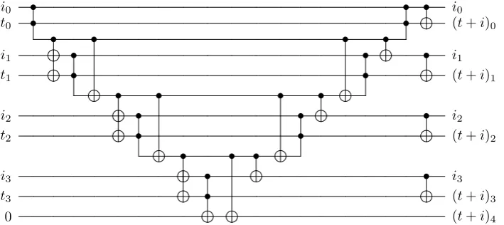
Note that the selected operations we need are similar to those in [8,63], and we can use a similar approach. The complexity is linear inN, and will therefore be smaller than the complexity of the state preparation. The technique is shown inFigure 1forselect1, andselect2is equivalent. If

p < q then theY operation inZ . . . ZY acts on the same qubit as one of theZs in theZ . . . ZX operation. As a result, the Y gets multiplied by Z and becomes ZY = −iX. Therefore the operation implemented is of the form −iXp,αZ . . . ZXq,α. If p > q then the X operation in Z . . . ZX acts on the same qubit as one of the Zs in the Z . . . ZY operation. Thus we have X times Z on that qubit giving XZ = −iY. Therefore the operation implemented is of the form

−iYpZ . . . ZYq. Ifp=q then all theZs cancel leaving onlyXp,αYp,α=iZp,α.

Now note that the register q1 is 0 for p > q and 1 for p < q. Before and after the ranged

operations, we perform an inequality test betweenpand q, controlled onq1, with the result that

an extra ancilla is in the state|1i unlessp=qand q1= 0. That register is used as a control for

the ranged operations, so ifp=qandq1= 0then the identity is performed. We then apply anS

zero, so the phase on the identity is unchanged. This yields the desired operations with the correct phases, and lastly the controlledZ on theθ register gives the(−1)θ1 _{phase factor.}

|1i ⊕p=q • S • ⊕p=q

control • • • • •

q1 Inq1

θ1 Inθ1 Z

plogN/−1 Inp =

logN−1

/ Inp Inp Inp

qlogN/−1 Inq

logN−1

/ Inq Inq Inq

α Inα Inα Inα

|ψi N/ select1

N

/ −→Z Yp,α

− →

Z Xq,α

Figure 1: The circuit needed to perform a controlledselect1 operation. We have omitted the registers this

operation does not act upon for simplicity. The unitaries labeled as−→Z Ajapply the operationZ0· · ·Zj−1Ajto

the target register, depending on the value from the input register, using the technique shown in Figure 9 of [8]. This operation can be achieved using an inequality test, followed by a ranged operation via the technique shown in Figure 8 of [8]. The controlled select2 operation is completely equivalent except with different control

registers.

4

Complexity

Let us denote the upper bound on the error required for the eigenvalue estimation by∆E. Then following [8] we find the complexity of the estimation is the cost of each LCU step times2m, where

m=

log

√_2πλ

2∆E

. (25)

Moreover, the error that is allowable for the implementation of each LCU step is

= √

2∆E

4λ . (26)

Some minor costs are as follows.

1. The cost of the controlled operation in Figure 1is 2N Toffoli gates for the two controlled ranged operations, and2dlogNefor the two inequality tests. These need to be done twice for a total of4N+ 4dlogNe.

2. In the state preparation we initially need to prepare superpositions over`, p, q, r, s, with `≤L,N/2> p≥q,N/2> r≥s. This can be achieved by creating an equal superposition over ranges that are powers of two using Hadamards, then flagging success using inequality tests. The number of Toffolis needed for these inequality tests will correspond to the number of qubits. Amplitude amplification can give the desired result with amplitude close to 1. The reflection in the amplitude amplification also needs a number of Toffolis corresponding to the number of qubits, so formsteps of amplitude amplification the number of Toffolis is3m+ 1

times the number of qubits. This needs to be multiplied by two because there is preparation and inverse preparation at each step.

4. For the state preparation we also do controlled swaps of the p and q, as well as r and s registers. These two controlled swaps cost2dlog(N/2)eToffolis.

5. Computing the function in Eq.(20)requires multiplication by a constant, a regular multipli-cation, and three additions. The division by 2 can be achieved by trivially shifting the bits. The multiplication can be achieved with2dlog(N/2)e2 _Toffolis.

In the remainder of this section we quantify the costs of the QROM needed for the state preparation, which is the main contributor to the complexity, then give the total cost.

4.1

RWSWT orbitals

The prominence of the RWSWT paper [29], which was the first work to rigorously estimate the T complexity of any quantum algorithm for chemistry makes it an important benchmark. Unfor-tunately, LLDUC [45] later argued that there were substantial problems with the orbitals chosen for the RWSWT paper. For the reasons discussed in the paper by LLDUC, we believe that future papers should compare against this work using only the LLDUC integrals. But in order to more easily compare with past work, here we analyze the complexity of simulating both RWSWT and LLDUC FeMoco active spaces. Note that at 152 spin-orbitals the LLDUC active space is also significantly larger than the 108 spin-orbital RWSWT active space.

Our approach is to chooseLby observing the effect of truncation on two different efficient clas-sical correlated approximate methods for molecular electronic structure: Configuration Interaction at the singles and doubles level (CISD) and Møller-Plesset perturbation theory to second order (MP2). For a review of both methods, see [52].

We perform CISD/MP2 on the exact Hamiltonian and then perform CISD/MP2 on the trun-cated Hamiltonian for various truncations and track the discrepancy. In Figure 2 we plot how the energies converge for both the RWSWT [29] and LLDUC [45] integrals. Specifically, we plot the correlation energy (the difference between the mean-field energy and the exact energy) for the

0 100 200 300 400

L -0.024 -0.012 0.000 0.012 0.024 ∆ Ec ( L ) [a . u . ]

MP2 CISD chem. acc.

0 100 200 300 400

L 1 2 3 4 λW [1 0 4a . u . ]

(a) 108 spin-orbital active space from RWSWT.

0 100 200 300 400

L -0.024 -0.012 0.000 0.012 0.024 ∆ Ec ( L ) [a . u . ]

MP2 CISD chem. acc.

0 100 200 300 400

L 0 1 2 3 λW [1 0 4a . u . ]

(b) 152 spin-orbital active space from LLDUC.

Figure 2: Top: difference∆Ec between truncated and untruncated correlation energy, for the FeMoco cluster

with MP2 and CISD methods (red, blue). The grey shaded region represents chemical accuracy; thus, for both active spaces we expectL = 200 is sufficient for our purposes. Bottom: λW as a function ofL. For

RWSWT [29], λT = 1,490 a.u., λV = 8,373 a.u. and the maximum value of λW is 34,552 a.u.; thus, we

reason that the mean-field energy converges much faster than the correlation energy and so it is easier to see the trend this way. In general, CISD and MP2 are very different methods and we would expect truncation to affect them differently. However, both methods appear well converged, for both RWSWT and LLDUC integrals, by L = 200. This gives us confidence that the exact ground state energy of the truncated Hamiltonian would also be consistent with the exact ground state energy of the untruncated Hamiltonian by this point. Accordingly, we choose 200 as the rank of our Coulomb operator. Note that the RWSWT and LLDUC integrals have very different properties, and so we assume it is a coincidence that both converge around the same value ofL.

For the integrals of RWSWT with this truncation we obtainλ= 36,042 a.u.(seeFigure 2). For both active spaces, we will focus on obtaining the standard “chemical accuracy”, corresponding to

∆E = 0.0016a.u. [52]. For the integrals of RWSWT, that gives ≈1.7×10−8. The output size for the QROM is approximatelylog(N2_{/) forN = 108, giving about 40. More specifically, the}

output size for the probabilities in the QROM is given by Eq. (36) in [8]. In that equation, only the first term is significant, giving

µ=

log

₂√_2λ

∆E

. (27)

That would giveµ = 26 bits, except we have three steps of state preparation, which means the number of qubits for the probabilities needs to be increased by 2 to µ= 28. With N = 108we need two registers of size dlog(N/2)e= 6, as well as two single qubit registers for the θ values, for a total of M = 42 qubits for steps 3 and 4. As we take L = 200, for step 1 (preparing the superposition over the` register), only 8 qubits are needed for`, for a total of36qubits output. We will use the QROAM for steps 3 and 4, as these steps have the dominant complexity.

4.1.1 Dirty ancillae

If we are attempting to minimize the number of qubits used, it is convenient to combine steps 1 and 3. That is, we use a state preparation over`, p, andq simultaneously, and output alt values for these three indices. Then there are only two steps of state preparation, and we can reduce the number of qubits for the keep probabilities toµ= 27. That means the state preparation has an output size ofM1 = 8 + 12 + 2 + 27 = 49. There will be M2= 41qubits used for the output in

step 4, because there is one fewer qubit for the keep probability.

If we use dirty qubits, then in the first state preparation we can use the N = 108 system registers as well as theM2= 41ancilla registers that will be used as output in the next step. We

can therefore takek= 4, which uses(k−1)M1= 147qubits, and fits within that size. Similarly, for

the second state preparation, we are able to use the output registers from the first state preparation as dirty qubits. The cost of the QROAM compute would be2dd/4e+ 12M. For the uncompute, we can takek= 128, giving cost2dd/ke+ 4k= 2dd/128e+ 512.

TakingL= 200givesd1= (L+ 1)(N2/8 +N/4) = 298,485for the first preparation, and Toffoli

cost

2dd1/4e+ 12M1+ 2dd1/128e+ 512 = 155,008. (28)

For the second state preparationd2=L(N2/8 +N/4) = 297,000, giving Toffoli cost

2dd2/4e+ 12M2+ 2dd2/128e+ 512 = 154,146. (29)

The total is 309,154. The minor costs result in another 1,534 Toffolis, for a total of 310,688 (see

Appendix E). We find that the number of qubits for the phase estimation is

m=

log

√

2πλ

2∆E

= 26, (30)

so we obtain an overall complexity (in terms of Toffolis)

2m×310688≈2.1×1013. (31)

4.1.2 Large ancilla count

Alternatively, we can use a large number of ancilla qubits in an attempt to minimize the Toffoli count. In the compute step it is optimal to takek= 64, and in the uncompute step it is optimal to takek= 512. The combined complexity of compute and uncompute for each step is then

dd/64e+ 63M+dd/512e+ 512. (32)

In this case it is better to use steps 3 and 4 as described above, with a separate state preparation for ` in step 1. Since there are three steps of state preparation, we should take M = 42. The Toffoli complexity for step 1 is only 200 using normal QROM. With thedvalues given above, we obtain a complexity 8,405 for step 3 and 8,379 for step 4. The minor costs are increased to 1,594. That gives an overall Toffoli complexity of

2m×18578≈1.2×1012. (33)

Altogether there are 3,024 qubits used (seeAppendix E).

4.2

LLDUC orbitals

An alternative active space for FeMoco was advocated for in [45]. This work argued that the active space Hamiltonian from RWSWT did not properly capture the electronic structure of FeMoco and was classically solvable. LLDUC introduced an alternative Hamiltonian for the FeMoco active space withN = 152 spin-orbitals. There it is found that λT = 3,446 a.u. andλW = 20,746 a.u., for a total of λ = 24,192 a.u. The smaller value of λ means that the number of qubits for the probabilities should beµ= 27 regardless of whether we merge steps 1 and 3 or not. Since N is larger than before, we now need one additional qubit for each of the orbital numbers, for a total ofM = 43qubits.

4.2.1 Dirty ancillae

Merging steps 1 and 3, the output size isM1= 51for the first state preparation, thenM2= 43for

the second state preparation. This time takingk= 4would use(k−1)M1= 153qubits for the first

state preparation and(k−1)M2= 129for the second, both of which are small enough to use other

qubits as dirty qubits. We again can takeL= 200which results ind1= (L+ 1)(N2/8 +N/4) =

588,126 for the first preparation andd2 =L(N2/8 +N/4) = 585,200 for the second preparation

(step 4). Usingk= 128 for the uncompute again yields a cost for the first preparation of

2dd1/4e+ 12M1+ 2dd1/128e+ 512 = 304,378. (34)

The cost of the second preparation is approximately

2dd2/4e+ 12M2+ 2dd2/128e+ 512 = 302,772. (35)

The total of the minor costs is 1,818 for a total of 608,968. This time we find thatlog(√2πλ)/(2∆E)

is very slightly larger than 25

log

√_2πλ

2∆E

≈25.0015. (36)

It would be unreasonably inefficient to round up tom= 26. Instead we can allow very slightly less error in other parts of the algorithm (which does not affect the complexity significantly because the algorithm depends on that error logarithmically) and takem= 25. Then we get a total cost

2m×608968≈2.0×1013. (37)

4.2.2 Large ancilla count

If we use a large number of ancilla qubits, we should again take theksizes as 64and 512 in the compute and uncompute steps, respectively. We again perform steps 1 and 3 separately for this approach. TheM will be 43for both steps 3 and 4. Then using dd/64e+ 63M +dd/512e+ 512

gives Toffoli costs13,560 and13,508for steps 3 and 4, respectively. This time the additional step of preparation needs 200 Toffolis for QROM. The minor costs are increased to 1,872, for a total of 29,140. That gives an overall complexity in terms of Toffolis

2m×29140≈9.8×1011. (38)

The total number of qubits is 3,143.

In summary, the Toffoli costs are as given inTable 1. In this table we have given approximate formulae including only the leading terms, and takenk= 4for the QROM compute circuits.

5

Exploiting sparsity in the Coulomb operator

Next we provide a strategy for further reducing constant factors when qubitizing the non-factorized quantum chemistry Hamiltonians. It is also possible to apply this strategy to the factorized form, but the result is worse for the case of FeMoco, so we will not address it here. This strategy will likely reduce the T complexity in practical situations, but only by constant factors. We focus on the form of the Coulomb operator

V = X

α,β∈{↑,↓}

N/2

X p,q,r,s=1

Vpqrsa†p,αaq,αa†r,βas,β, (39)

which has the truncated form

e

V(c)= X

α,β∈{↑,↓}

N/2

X p,q,r,s=1

e

V_pqrs(c) a†_p,αaq,αa†r,βas,β, Ve_pqrs(c) = (

Vpqrs, |Vpqrs| ≥c,

0, |Vpqrs|< c.

(40)

The purpose of this truncation is to induce sparsity in the operators by removing near-zero elements. The idea of reducing quantum simulation costs by exploiting sparsity in the Coulomb operator was first explored in [64], but in the context of Trotter based methods. The idea of the approach here is to choose the value of c to be as large as possible while still leaving classical correlated approximations such as CISD within chemical accuracy (essentially the same procedure we used for choosingLshown inFigure 2). This is shown inFigure 3.

We will define L(_Vc) as the number of nonzero values of Ve

(c)

pqrs. In general, we expect that L(_Vc)=O(N4); which is to say that this truncation should not asymptotically change the sparsity of the operators. However, in practice we do expect to find thatL(_Vc) < N4_{/16; which is to say}

that we do expect there to be additional sparsity in these operators. While the matter of exactly how much sparsity exists is highly system dependent, we might sometimes desire an algorithm that exploits this sparsity, even if it is highly unstructured.

It is possible to perform a state preparation that has cost dependent on the number of nonzero elements, at the cost of a slightly larger number of ancillae. Consider the state preparation of [8], which has the following steps.

1. Create an equal superposition over the system registers

1 √

d d X j=1

|ji. (41)

2. Use QROM indexed on the system registers to output alt values and keep values

1 √

d d X j=1

-0.005 0.000 0.005 0.010

∆

E

(

c

)

[a

.

u

.

]

MP2 CISD chem. acc.

10−8 ₁₀−7 ₁₀−6 ₁₀−5 ₁₀−4 ₁₀−3

c[a.u.] 106

107

L

(

c

)

V

(a) 108 spin-orbital active space from RWSWT.

-0.015 -0.010 -0.005 0.000 0.005

∆

E

(

c

)

[a

.

u

.

]

MP2 CISD chem. acc.

10−8 ₁₀−7 ₁₀−6 ₁₀−5 ₁₀−4 ₁₀−3

c[a.u.] 105

106

107

108

L

(

c

)

V

(b) 152 spin-orbital active space from LLDUC.

Figure 3: We show the result of performing the truncation of Eq.(40). Top: we show difference∆E(c)between truncated and untruncated correlation energy, for the FeMoco cluster with MP2 and CISD methods (red, blue) as a function of thecparameter in Eq.(40). The grey shaded region represents chemical accuracy. Bottom:

L(c)_V as a function of c. For RWSWT [29], we can safely truncate at c = 0.0002 a.u., which corresponds to L(c)_V = 3,300,568. For LLDUC [45], we can safely truncate at c = 0.0001 a.u., which corresponds to

L(c)_V = 1,291,648.

3. Use another ancilla in an equal superposition over2µ _{values whereµis the number of digits} for keep. Perform an inequality test between this register and the keep register, and swap the contents of the first two registers (the index and alternative index registers) based on the result of this inequality test.

The total number of ancillae used by this state preparation is2dlogde+ 2µ+ 1.

In order to perform the preparation in the sparse case, instead of iterating over the index register, we can output the index register in the same way as the alternate index register. That is, we have a register which iterates over the number of nonzero amplitudes in the state we aim to prepare. Denoting that numberd, our steps are as follows.

1. Create an equal superposition over the register indexing the nonzero entries.

1 √

d d X j=1

|ji. (43)

2. Use QROM indexed on this first register to output ind, alt, and keep values

1 √

d d X j=1

|ji |indji |altji |keepji. (44)

3. Use another ancilla in an equal superposition over2µ values, and perform an inequality test between this register and the keep register. Based on the result of this inequality test, swap the contents of the ind and alt registers.

follows immediately from the correctness of the routine in [8], because after the QROM lookup the state in the registers excluding the first is equivalent to that in [8]. The Toffoli complexity of this modified state preparation procedure for sparse states depends on the number of nonzero entries rather than the dimension.

For our application, the non-factorized form of the Hamiltonian with truncation of the Coulomb operator can be expressed using the Jordan-Wigner representation. Using Eq. (2) and the sym-metriesTpq=Tqp,Vpqrs=Vqprs=Vpqsr, the Hamiltonian can be written as

H =1 2 X σ∈{↑,↓} N/2 X p,q=1

Tpq(a†p,σaq,σ+a†q,σap,σ)

+1 4 X α,β∈{↑,↓} N/2 X p,q,r,s=1

Vpqrs(a†p,αaq,α+a†q,αap,α)(a†r,βas,β+a†s,βar,β). (45)

Then using the Jordan-Wigner representation via Eq.(8)and truncatingV, the Hamiltonian can be represented as

H 7→ X

σ∈{↑,↓}

N/2

X p,q=1

TpqQpqσ+ X α,β∈{↑,↓} N/2 X p,q,r,s=1 e

Vpqrs(c) QpqαQrsβ, (46)

where

Qpqσ=     

Xp,σZX~ q,σ, p < q, Yp,σZY~ q,σ, p > q,

1

2(1−Zp,σ), p=q.

(47)

Here we have again used the symmetriesTpq=Tqp,Vpqrs=Vqprs=Vpqsr. Usingp < qversusp > q to distinguish between Xp,σZX~ q,σ and Yp,σZY~ q,σ is a convenient way to perform the controlled operations as described inFigure 1. This is of the form of a linear combination of unitaries, and the state we need to prepare is of the form

|0i |+i |0i |0i X

σ∈{↑,↓}

N/2

X p,q=1

r

|Tpq| λ |θ

T

pq00i |p, q, σi |0i

+|1i |+i |+i |+iX

α,β∈{↑,↓}

N/2

X p,q,r,s=1

s

|Ve

(c)

pqrs| λ |θ

V

pqrsi |p, q, αi |r, s, βi. (48)

The first register is just a convenient replacement for the|`i register, and is used to distinguish between the one and two body terms. The second register is used to distinguish between1andZp,α forp=q, and the third register is used to distinguish between1andZr,β forr=s. The second, third, and fourth registers will be used to generate the symmetries of the state. The fifth register is used to give the appropriate sign of theTpqandVe

(c)

pqrsweightings, which are now combined instead of having two separate registers as before.

We can again use symmetry to reduce the number of coefficients that need to be prepared. For Vpqrs there is symmetry between exchangingp andq, between exchanging rand s, and between exchanging thep, q and r, spairs, as described in Eq. (5). ForTpq there is symmetry between p andq. For this reason we will initially only prepare amplitudes forp≤q,r≤s, andp≤rforV, andp≤qforT.

To simplify the description, we will introduce some notation,

ζpq:=      √

2, p < q,

1, p=q,

0, p > q.

We will also allowζ to be used with four subscripts, which means

ζpqrs:=      √

2, pq < rs,

1, pq=rs,

0, pq > rs,

(50)

where the notationpq < rsindicates that eitherp < r orp=randq < s, andpq=rsindicates thatp=randq=s. That is, if these are the composite indices for the matrix W, thenpq < rs indicates the upper triangle, andpq=rsindicates the diagonal.

In terms of this notation, the state produced will initially be

|0i |+i |0i |0i X

σ∈{↑,↓} N/2 X p,q=1 ζpq r

|Tpq| λ |θ

T

pqi |p, q, σi |0i

+|1i |+i |+i |+i X

α,β∈{↑,↓}

N/2

X p,q,r,s=1

ζpqζrsζpqrs s

|Ve

(c)

pqrs| λ |θ

V

pqrsi |p, q, αi |r, s, βi. (51)

Usingζ ensures that the number of nonzero terms is about1/2 as much forT, and about1/8 as much for V. These sparse entries can be prepared by the technique described above for sparse state preparation. ForT the only terms prepared here are those wherep≤q, and forV only where p≤q,r≤s, and pq≤rs. Next we perform three steps.

1. Swap thep, qandr, sregisters controlled on the state of the fourth register.

2. Swap thepandqcontrolled on the state of the second register.

3. Swap therandscontrolled on the state of the third register.

To show the effect of this, we will first show it for the first component of the state, with0in the first register and weightings dependent onT. The first and third controlled swaps have no effect because third and fourth registers are zero. The second controlled swap gives us

|0i |0i |0i |0i X

σ∈{↑,↓} N/2 X p,q=1 ζpq r

|Tpq|

2λ |θ T

pqi |p, q, σi |0i

+|0i |1i |0i |0i X

σ∈{↑,↓} N/2 X p,q=1 ζpq r

|Tpq|

2λ |θ T

pqi |q, p, σi |0i

=|0i |0i |0i |0i X

σ∈{↑,↓} N/2 X p,q=1 ζpq r

|Tpq|

2λ |θ T

pqi |p, q, σi |0i

+|0i |1i |0i |0i X

σ∈{↑,↓} N/2 X p,q=1 ζqp r

|Tpq|

2λ |θ T

pqi |p, q, σi |0i

=|0i X

σ∈{↑,↓}

N/2

X p,q=1

r

|Tpq|

2λ (ζpq|0i+ζqp|1i)|0i |0i |θ T

pqi |p, q, σi |0i

=|0i X

σ∈{↑,↓}

N/2

X p,q=1

r

|Tpq| λ |κpqi |θ

T

pqi |0i |0i |p, q, σi |0i, (52)

where we have defined the state labelling

κpq:=     

0, p < q,

1, p > q,

+, p=q.