Tuning Parallel SAT Solvers

EPiC Series in Computing

Volume 59, 2019, Pages 127–143

Proceedings of Pragmatics of SAT 2015 and 2018

Tuning Parallel SAT Solvers

Thorsten Ehlers

and Dirk Nowotka

Department of Computer Science University of Kiel

{the,dn}@informatik.uni-kiel.de

Abstract

In this paper we present new implementation details and benchmarking results for our parallel portfolio solver TopoSAT2. In particular, we discuss ideas and implementation details for the exchange of learned clauses in a massively-parallel SAT solver which is designed to run more that 1,000 solver threads in parallel. Furthermore, we go back to the roots of portfolio SAT solving, and discuss the impact of diversifying the solver by using different restart- , branching- and clause database management heuristics. We show that these techniques can be used to tune the solver towards different problems. However, in a case study on formulas derived from Bounded Model Checking problems we see the best performance when using a rather simple clause exchange strategy. We show details of these tests and discuss possible explanations for this phenomenon.

As computing times on massively-parallel clusters are expensive, we consider it espe-cially interesting to share these kind of experimental results.

1

Introduction

The satisfiability problem of propositional logic (SAT) has attracted large interest in recent decades. It is used in a wide field of applications, such as planning and scheduling [3, 22,19], the verification of hardware and software [17], computation of tree decompositions [13, 11]. For example, it can be effectively used to design optimal sorting networks [24] or solve the pythagorean triple problem [35]. Furthermore, it is the underlying technique for MaxSAT [39], SMT [41] and some CP solvers [43].

The increasing availability of parallel hardware has raised interest in the parallelization of SAT solvers [31, 26]. However, there are principle considerations on the problem of SAT solving which have provoked some skepticism about parallel SAT solvers. Wintersteiger posed challenges for parallel SAT solving [32]. Katsirelos et al. analyzed the structure of the proofs that SAT solvers generate for unsatisfiable formulas, and gave some evidence that these proofs have an inherently sequential structure which prevents parallel SAT solvers from scaling up [36]. Nevertheless, nowadays even most laptops come with multi-core CPUs, and it is likely that hardware will become more and more parallel. Thus, it makes sense to push SAT solvers to

∗_{This work is partially funded by the German Federal Ministry of Education and Research, combined project}

benefit as much as possible from this hardware. 6 Parallel SAT solving is challenging, but some of these challenges can be tackled by a well-designed parallel SAT solver. Furthermore, the existence of proofs which cannot be created in parallel efficiently does not imply that all proofs cannot be parallelized efficiently. Here, we take the perspective of Gustafson’s Law [30] rather than Amdahl’s Law [2]. We show that using more parallel hardware does not only come with some speedup, it also allows for solving larger and harder problems, e.g. for analyzing larger systems. We claim that this is a realistic perspective: Whenever better solvers are available, they will not only be used to solve the same problems faster. Users tend to use these solvers to tackle harder and larger problems. If these problems are sufficiently hard, we give evidence that in many cases significant speedups can be observed on parallel SAT-solvers; in this particular case up to 1536 solver threads. et al. This paper is structured as follows. After an overview over SAT and related work, we describe the design decisions made in our parallel solver, and relate it to the design of both sequential and parallel SAT solvers. Then, we present a case study on formulas from bounded model checking which demonstrates the scaling of our parallel solver in the spirit of Gustafson’s law. Finally, we show that the scaling translates to a wider range of problems and conclude.

2

Background

Given a propositional formulaϕ, the satisfiability problem asks whether there is an assignment of the variables ofϕto true and false which satisfies the formula, or not. Formulas are usually given in conjunctive normal form. That is, a formulaϕis given as a conjunction of disjunctions of literalsVn

i=0Ci, whereCi, called clause, is given as Ci= W|Ci|

j=1`i,j and`i,j, called literal, is either a boolean variablexor its negation ¯x. A clause is satisfied by an assignmentβif at least one of its literals is assigned to true, and the formula is satisfied if all its clauses are satisfied. For every propositional formula there exists an equisatisfiable formula in conjunctive normal form, and the formula can efficiently be transformed to conjunctive normal form [47].

A clauseC is implied by a formulaϕif every satisfying assignment forϕalso satisfiesC. Given two clauses C1 = (x∨A) and C2 = (¯x∨B) where A and B are disjunctions, the clause (A∨B) can be derived as resolvent ofC1andC2 by the resolution rule. This resolvent is implied by the original formula, and may thus be added to it without changing the formula’s satisfiability. A formula is unsatisfiable, if, and only if, the empty clause can be derived by repeated application of the resolution rule [45].

In this paper we focus on complete solvers rather than other, incomplete solvers as they are often used e.g. for solving random formulas. These SAT solvers run a significantly improved version of the DPLL algorithm [20]. Once the solver reaches a situation in which it has to backtrack, it analyzes the reason for this failed search, and stores it in a new, learned clause [40]. This algorithm is often referred to as Conflict-Driven Clause Learning (CDCL) and prevents the solver from repeatedly searching similar parts of the search space. The derivation of learned clause can be explained as a sequence of resolution steps. Thus, the proof of unsatisfiability that CDCL solvers create is a resolution proof. Furthermore, it has been shown that clause learning is as powerful as general resolution [12].

An important notion in this context is the Literal Block Distance (LBD) of learned clauses. As a sophisticated extension of the DPLL algorithm, SAT solvers basically run a backtracking search. Assume the solver branches some variablex1 to false, and there is a clause (x1∨x2). Then, x2 must necessarily be set to true, as otherwise this clause would be falsified. After each branching, the solver runs a propagation routine which identifies such situations, and propagates variable assignments with respect to previous branches. Variable assigned after the i−thbranching step are said to lie on decision leveli. The LBD measure counts the number of different decision levels occurring in a learned clause. It has empirically been found that clauses with low LBD value tend to be especially useful for the solver.

There are basically two approaches to parallelize SAT solvers. Firstly, given a formula φ containing a variablex, the search space can be divided intoφ∧xandφ∧x. Then, two solvers¯ can be run on the two subformulas. In case more parallel hardware is available, this splitting process is repeated recursively. If one of the subformulas is satisfiable, so isφ, and otherwise φis unsatisfiable. The conjunctions which determine the subformulas are often called guiding paths. When combined with sophisticated look-ahead techniques for finding good branching literals, this approach is also called Cube&Conquer [33]. Here, the challenge is to split the search space such that the subformulas become easy to solve, and the search tree is somewhat balanced.

Secondly, the performance of sequential SAT solvers tends to be volatile with respect to parameters like the initial variable ordering. In parallel portfolio SAT solvers, several instances of sequential SAT solvers are run in parallel, each of them with different parameters. The solver which terminates first wins, and its result is reported. Thus, these solvers take advantage of the volatility of the performance of sequential solvers. The first portfolio solver was ManySAT [31]. In addition to the diversified search obtained from running the solvers with different param-eters, the solver instances collaborate by exchanging learned clauses. This is sound as every learned clause was derived by resolution, and thus is logically implied by the original formula. This clause exchange is crucial in improving the performance of parallel SAT solvers, especially on unsatisfiable formulas [26,10].

In this paper, we follow the portfolio approach, which is the technique used by most parallel SAT solvers nowadays.

3

Solver Design

When designing a solver which is meant to scale beyond 1000 solver threads running in parallel, several issues arise. Firstly, whenever one of the solver threads learns a new clause, a decision has to be made whether or not this clause is shared with other solver threads.

Secondly, an efficient mechanism is needed to dispatch shared clauses among the solver threads. This concerns both communication on shared memory systems, where locking is a potential bottleneck, as well as inter-process communication, e.g. by MPI. Thirdly, whenever a solver thread receives a clause, a strategy is needed to decide if and how long this clause should be stored. The strategies for sending and receiving clauses interact: If, in a massively-parallel setting, many clauses are sent, then a more aggressive mechanism to select or delete received clauses is needed. These questions are posed as challenge in [32].

Fourthly, some techniques which are sufficiently fast for a sequential SAT solver may be too slow for a parallel SAT solver. For example, if a preprocessor is used then the overall solving timeT =Ts+Tpre is the sum of the time required by the preprocessorTpre and the time for

Our solver is based on Glucose 3.0. In Glucose, the preprocessor works well on many formulas, but is very slow especially if there are many large clauses, or if some clauses are put on the subsumption queue repeatedly. Instead of using a (non-deterministic) parallel BVE algorithm [29], we improved upon the preprocessor from Glucose by implementing linear-time versions of the subsumption check and the resolution of two clauses, similar to the algorithm used in Cadical [16]. Furthermore, we equipped the clause headers with a boolean flag which indicates whether a clause already is on the subsumption queue or not.

Although Glucose 3.0 is not the fastest available sequential solver, its clear structure makes it easy to modify it for testing parallel implementations. Furthermore, it uses less heuristics than other solvers, which makes its performance more stable with respect to modifications.

3.1

Communication

In order to achieve an efficient communication, we use a hierarchical architecture. Our solver runs several MPI processes, each of which runs one thread for communication, and several solver threads. The communication between processes is performed asynchronously. Processes send their learned clauses either if some time has passed since the last sending operation, or if their clause buffer is sufficiently full. Compared to the communication strategy of HordeSAT [10] where communication is performed synchronously and the amount of transmitted data is re-stricted to 1500 integers per process and communication cycle, our strategy allows us to send a larger number of clauses in situations where many good clauses are learned. By collecting several clauses before sending them we prevent the network from being congested by a large number of small messages. Furthermore, sending messages asynchronously avoids peaks in the network usage.

Inside each process, we use a bug-fixed version of the lockless clause sharing mechanism from ManySAT [31]. The fix was necessary because the original implementation could cause the solver to report “satisfiable” on unsatisfiable formulas.

Compared to the distributed version of Syrup [5] which uses locks in its shared memory communication, this lockless implementation avoids a potential bottleneck.

Whenever a solver thread learns a good clause, it may copy it to the input buffer of the communication thread. The communication thread regularly checks these buffers, and copies their content to its MPI buffer. Similarly, clauses received via MPI are dispatched through buffers in the shared memory.

There are formulas on which the solvers threads learn a huge number of unit clauses, i.e. clauses of size 1, in the very beginning of the solving process. In order to reduce the traffic in such cases, each communication threads stores the unit clauses it has seen already. When receiving unit clauses either from other processes via MPI or from solver threads via the shared memory communication, it checks these clauses against the clauses it has seen already, and only forwards unit clauses which have not yet been seen. In other solvers like TopoSAT [26] and HordeSAT [10], the communication threads hash clauses received either from solver threads within the same process or via MPI. They use Bloom filters for preventing clauses from being shared multiple times. We found that these filters only remove a small portion of the sent clauses in most cases and most configurations we used. Furthermore, they only identify identical clauses and fail e.g. in identifying subsumed clauses. As we were interested in the structure of the clauses which are exchanged, we did not use any filter in these experiments. Instead, we regularly checked the stored clauses for duplicates, and identified some paticular solver configurations which lead to a large number of duplicate clauses.

are regularly checked for subsumption.

3.2

Sending Clauses

We implemented different strategies for deciding whether or not to share a clause. The first strategy simply considers the LBD value of the learned clauses, and shares clauses if this value is sufficiently low. In our experiments, we used a threshold of 4.

Audemard et al. [8] suggested to defer the sharing of a clause until it has been used by the solver for a second time. This strategy is based on the observation that many learned clauses are not helpful in the subsequent solving process. In our second sharing technique, we lifted this approach to the next higher level in our solver’s hierarchy. Whenever a solver thread learns a clause, it can be sent to other solver threads within the same process. These solver threads monitor the usage of received clauses, and notify the communication thread whenever a received clause has been used for the first time in conflict analysis. Once a certain threshold of usages has been reached, the communication thread can decide that this clause is likely to be actually helpful for other solvers, and send it to other processes via MPI. This is implemented by storing both the clause and an unique identifier in the communication thread.

The third approach is inspired by the concurrent clause strengthening solver by Wieringa et al. [48]. Their solver runs a solver thread and a so-called reducer thread in parallel. Whenever the solver thread learns a clause, this is sent to the reducer thread, which in return tries to find a subsuming clause. Similar to the clause vivification process from [44], this is done by assuming the negation of the clause, and using the analyzeFinal-method from MiniSAT [23] to try to compute a subsuming clause. From the proof perspective, this process can be seen as the repeated application of the resolution rule. If successful, i.e. if a clause was found which is actually shorter than the original one, this one is sent back to the solver thread. Instead of using a dedicated reducer thread, we let solver threads store learned clauses in a dedicated buffer instead of sending them immediately. On the next restart, search is interrupted and the solver thread tries to minimize each of the stored clauses before sending them. A similar idea is presented in [38] in order to strengthen clauses in the learnt clause database of a sequential solver. The rationale behind this approach is that after learning the clause, the solver has backtracked and continued its search in a similar part of the search space. Thus, it is likely that is has learned more clauses which help in the minimization process. Furthermore, the time used for strengthening clauses must be limited. Thus, using this approach on the receiving side would not scale, as the amount of clauses which are exchanged within the solver grows with the parallel resources used.

3.3

Handling Received Clauses

Audemard et al. suggest to “freeze” learned clauses if they have not been used for while, instead of deleting them immediately [4]. In a parallel setting, they lift this approach to received clauses [8]. Oh uses a different approach in his award-winning solver COMiniSatPS [42]. Here, clauses with a sufficiently low LBD value are kept forever, whereas clauses with larger LBD are kept in a separate database. These clauses are removed if they have not been used by the solver for some time. As this approach is quite successful in a sequential setting, we adapted it for our parallel solver. Assume a parallel solver with 1000 solver threads, where every threads shares only 2% of its learned clauses. Then, each solver threads receives 20 times more clauses from other solvers than it produces itself. This is both curse and blessing for the receiving solver: It is faced with a huge amount of clauses from which it may pick those that are likely to help in the subsequent solving process. On the other hand, it cannot store all of them as this would significantly harm the propagation speed, and in the worst case the solver may run out of memory.

Thus, we decided to modify Oh’s approach for this setting. Whenever a clause is received, its LBD value is initially set to the size of the clause, as this is a trivial upper bound. If the solver thread uses this clause, the LBD value may be updated, i.e. decreased. If this decrease is strong enough, the clause is transfered to a permanent storage. Received clauses which are not used within an interval of 30,000 conflicts are deleted.

3.4

Improved Diversification

The core idea behind the first portfolio solvers was to speed up the solving process by diversifying different parameters of the individual solvers. After a while in which clause exchange was the dominant topic, this diversification receives more attention again.

For example, the competition version of Painless [27] diversifies search by choosing different initial phases for the variables, and using LRB on some, and VSIDS on the other solver threads. ABCD SAT [18] chooses some literals which occur often, and diversifies the individual search spaces of the solver threads by pinning them to the subformulaφ∧`i. Furthermore, it diversifies

its clause database management and sometimes uses the size of clauses rather than their LBD as parameter, as suggested in [25].

In_TopoSAT2, we decided to use three basic techniques as source for some diversification. Some solvers use VSIDS as branching technique, whereas others use LRB. We use the adaptive restart technique from Glucose [7], Luby restarts as in MiniSAT, and inner-outer-restarts [14] on some of the cores. Furthermore, some threads use the default clause database management scheme of Glucose, whereas others use several clause databases for permanent, received and other clauses as discussed in the previous section. We ran some experiments with sequential versions of Glucose to figure out combinations which work well. For example, combining LRB with the adaptive restarts of Glucose did not work very well, thus we only use LRB in com-bination with Luby and inner-outer restarts in our portfolio. We consider this diversification especially helpful when the solver is run on unknown formulas. However, in the case study in Subsection4.1we did not use it, as VSIDS and Glucose restarts worked well together on these formulas.

4

Experimental Results

4 nodes. Therefore, the configurations for which we present results here used multiples of 24·4 = 96 threads. On each node, we ran 3 processes with 8 solver threads each. The interconnect in this cluster has a latency of 2µs, and each node can receive a traffic of at most 10GiB/s1_.

Next, we discuss a case study on formulas from bounded model checking. Afterwards, some results on benchmarks from the SAT Competition 2016 are presented.

4.1

Case Study: Bounded Model Checking

Bounded Model Checking (BMC) is a technique applied to finding bugs in both software and hardware [17]. Given a transition systemM with a countable setSof states and a finite number of successors for each state, let the predicateI(s0) denote the finite set of initial states and the predicate T(si, si+1) denote the transition relation, where sj ∈ S for allj ≥ 0. Let P(s) be

a predicate which propositionally defines a set of error states. One can check if such an error can be reached withinksteps by “unrolling” the transition relationk times, and checking the satisfiability of the formula

ϕk= I(s0)∧

k−1 ^

i=0

T(si, si+1)∧P(sk)

Clearly, this formula translates to a propositional formula for any transition system M and predicateP as specified above. Ifϕk is satisfiable, then its satisfying assignment describes a

path of lengthkfrom an initial state to an erroneous state, allowing e.g. developers to identify the reason for this behavior, and fix it. Bounded Model Checking is an incomplete verification procedure since a negative result either means that the system is safe or thatkwas chosen too small. Thus, it is important to check sufficiently large values ofk.

This gives rise to the following questions: Given parallel hardware, can we check the unsat-isfiability ofϕk faster for some fixed value of k? And, according to Gustafson’s Law and even

more importantly, can we check this for larger values ofkwithin a reasonable amount of time? In this case study, we chose formulas which describe safety properties of the french railway system [37]. Here, the unroll depths range from 7 to 15. The unroll depth required for a meaningful analysis is highly problem-dependent, in this case, such small numbers were already sufficient. Each of these formulas is unsatisfiable. Thus, they allow for a good evaluation of the scaling of our solver when creating large resolution proofs. We begin by presenting some results of a rather simple solver setup. Then, we show that these results can be improved quite easily, and discuss some statistics which may explain why the solver scales up rather nicely in this case.

As a first setup, we used the simple LBD-based clause sharing scheme. The solvers shared clauses of LBD at most 4, and stored clauses permanently if their LBD was updated to a value of at most 3. The results from running our solver on these formulas are depicted in Table 1. The first columns shows the unroll depth, followed by the running times for 96 up to 1536 threads. The last columns give the speedups when comparing 96 to 1536 threads and 768 to 1536 threads, respectively. This table contains both positive and negative results. On the negative side, the scaling on the smallest instance is limited. Here, the solving times are reduced by only a factor of 2.05 when using 1536 instead of 96 threads. Thus, this formula may be too easy for the parallel solver in the sense that scaling is prevented by some inherent sequential structure of the proof of unsatisfiability.

Table 1: Scaling on Bounded Model Checking Benchmarks. Here, a timeout of 4 hours was used. The running times are given in seconds.

# Threads Speedups

Depth 96 192 384 768 1536 96 vs. 1536 768 vs. 1536

7 250 198 163 137 122 2.05 1.12

8 414 319 247 219 182 2.27 1.20

9 882 496 387 347 269 3.28 1.29

10 1680 923 581 456 376 4.46 1.21

11 10574 5641 3149 1960 1360 7.78 1.44

12 T/O 9890 5765 3439 2064 — 1.66

13 T/O T/O 9419 5422 3166 — 1.71

15 T/O T/O T/O 11845 6749 — 1.76

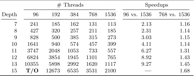
Table 2: Scaling on Bounded Model Checking Benchmarks. Here, a timeout of 4 hours was used. The running times are given in seconds. Here: Preprocessing is used!

# Threads Speedups

Depth 96 192 384 768 1536 96 vs. 1536 768 vs. 1536

7 241 185 162 131 113 2.13 1.16

8 427 320 257 211 185 2.31 1.14

9 828 500 385 315 273 3.03 1.15

10 1641 940 574 457 399 4.11 1.14

11 3747 2048 1053 733 557 6.27 1.31 12 6824 3854 1945 1101 765 8.92 1.43 13 10355 5898 2992 1620 1117 9.27 1.45

15 T/O 12673 6535 3531 2100 — 1.68

However, the harder the formulas become, the more parallelism pays of. The speedup obtained from using 1536 instead of 96 threads increases from 2.05 to 7.78, until the smaller solver instances cannot solve the benchmarks anymore. Similarly, the performance gain when moving from 768 to 1536 threads increases, and reaches a maximum value of 1.76 on the hardest formula.

In the bigger picture, we see a triangle of timeouts on the left, lower part of Table1. This triangle shows that whenever we double the amount of hardware we use, this immediately implies that a deeper analysis can be performed within the time limit of 4 hours. Using parallel hardware does not only allow for running the analysis for some fixed unroll depth kfaster, it especially allows for checking harder formulas, thus finding bugs which are hidden deeper in the system, or, if no such bugs are found, increase the trust in the correctness of the system under analysis.

0 1 2 3

·106

0 0.5 1 1.5 2 2.5

·106

# conflicts permanent

local received

0 0.2 0.4 0.6 0.8 1

·106

0 0.5 1 1.5 2 2.5

·106

# conflicts permanent

local received

0 2 4 6

·105

0 0.5 1 1.5 2 2.5

·106

# conflicts permanent

local received

Simple, 192 Threads, 12673s Simple, 384 Threads, 6535s Simple, 768 Threads, 3531s

0 1 2 3

·106

0 1 2 3

·106

# conflicts permanent

local received

0 0.5 1 1.5 2 2.5

·106

0 1 2 3 4

·106

# conflicts permanent

local received

0 0.2 0.4 0.6 0.8 1 1.2 1.4

·106

0 1 2 3 4 5·10

6

# conflicts permanent

local received

Lazy, 192 Threads, T/O Lazy, 384 Threads, 10626s Lazy, 768 Threads, 5578s

Figure 1: Test on the formula sncf model ixl bmc depth 15.cnf: Number of clauses in the different clause storages before the empty clause was derived.

For example, the formula for unroll depth 15 can be solved in 6535 seconds on 384 threads now, compared to 6749 seconds on 1536 threads before. Although this is not a technical contribution, we consider this interesting as it shows that instead of only focussing on the parallelisation aspect, one should still keep an eye on such issues. Still, the speedups are significant, especially on the hard formulas. For example, increasing the number of threads by a factor of 8 from 192 to 1536 threads yields a speedup of 6.03 on the hardest formula. We consider these results quite interesting. Unfortunately, it prove hard to improve upon then. Thus, the question arose why this configuration works this well. A possible hint is depicted in Figure1. This figure shows statistics on the clause databases of_TopoSAT2when running on the formula “sncf model ixl bmc depth 15.cnf”. Whenever the clause database was reduced, we recorded the size of the different clause storages. Permanent denotes the size of the database for clauses with LBD at most 3. Additionally, the running times are given.

In the first row results are given for the simple, LBD-based clause exchange policy. Inter-estingly, the size of the permanent storage rises to values slightly below 2.5·106 clauses before UNSAT is found. In some cases, this number drops at the end of the solving process as many unit clauses are found here.

This number is more or less stable, no matter how many solver threads are used. For space reasons we omitted the results for 96 and 1536 threads. These results may be seen as a partial explanation of why the solver scales so well here: If many clauses were exchanged and stored which do not help in deriving the empty clause, then the final size of the database for permanently stored clauses should increase when more parallel solvers are used.

0 0.5 1 1.5 2 2.5 3

·105

0 0.5 1 1.5 2 2.5·10

6

# conflicts permanent

local collisions

0 2 4 6

·105

0 1 2 3 4 5

·106

# conflicts permanent

local collisions

0 0.5 1 1.5 2

·105

0 0.5 1 1.5 2 2.5·10

6

# conflicts permanent

local collisions

Simple exchange Lazy exchange Exchange with strengthening

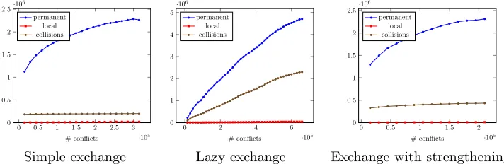
Figure 2: Size of clause databases and number of duplicate clauses when solving the formula sncf model ixl bmc depth 15.cnf with 1536 threads and different export strategies.

the respective clause databases are shown in the lower row of Figure1. The number of deleted clauses is significantly lower. However, the final size of the clause database increases with the number threads we used. Compared to the first row with results for the simple clause exchange policy, the running times are significantly larger.

We conjectured that the problem here might be that the time between learning and transfer-ring good clauses might be too large, and thus redundant clauses would be learned. If identical clauses would be learned and transmitted, this might be captured by using e.g. Bloom Filters as suggested e.g. in [10].

Instead of hashing clauses during import, we checked for duplicates whenever the clause DB was reduced. In this way, we can also capture whether duplicate clauses remain in the clause database for a long time, or if they are removed frequently, e.g. because the are satisfied by top-level assignments. Furthermore, this can be done pretty efficiently, and hardly influences the solving process. Table 2 exemplifies results for the hardest of the formulas in this case study. Here, collisions denotes the number of collisions of hash values, thus it is an upper bound on the actual number of duplicates. For three different export-strategies, it shows both the development of the size of the clause database and the number of duplicates in it. In the simple export strategy where clauses are exported immediately, the solvers learn some duplicate clauses in the beginning of the solving process. However, this number is quite low, and stays stable over the time. Contrary, the second chart shows the number of duplicate clauses when using lazy clause export. Here, the number of duplicates is significant, and grows over the time. The third chart presents the configuration which strengthens clauses before export. With this setup, there are slightly more collisions that in the first setting, but the number is still quite low. The findings from this experiment are two-fold. Firstly, Bloom filters do make sense especially if the transfer of learned clauses is slow, either because of lazy exchange policies or because of a slow interconnect, e.g. in a distributed environment. Still, duplicate clauses mean that redundant work was performed. Thus, filtering with a Bloom filter only prevents storing duplicates, but not this redundant work. It appears therefore important to exchange learnt clauses fast.

Table 3: Overall traffic via MPI in MB Depth Simple Exc. Lazy Exc.

7 11658 966

8 14261 1737

9 18841 2552

10 22620 4286

11 25245 6408

12 34553 8522

13 37287 11124

15 56531 17189

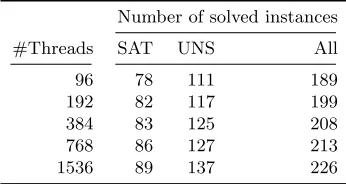
Table 4: Simple Clause Exchange

Number of solved instances

#Threads SAT UNS All

96 78 111 189

192 82 117 199

384 83 125 208

768 86 127 213

1536 89 137 226

which could be strengthened by self-subsuming resolution was small compared to the overall number of clauses. It would be interesting to see if this works out better on other formulas.

However, the lazy configuration has one major advantage. Table3shows the amount of data sent via MPI for different unroll depths and configurations, each using 768 threads. Especially for easier formulas, the network traffic is significantly lower with the lazy clause exchange. This amount of traffic is no problem for clusters with high-performance interconnect, but may be an issue when using e.g. cloud computing.

4.2

SAT Competition 2016 Benchmarks

In order to check the applicability of our solver on a wider range of formulas, we chose bench-marks which were used in the application track of the SAT competition 20162_{. This benchmark} set covers a wide range of different applications. In the competition, the best sequential solver could solve 154 of these benchmarks within a time limit of 5000 seconds (70 SAT, 84 UNSAT). The solvers were quite close, the solver which was ranked 5th solved only 4 instances left.

A virtual best solver (VBS) is a hypothetial solver which, when run on one for the formulas, would choose the best-performing solver out of the 27 competitors for this particular bench-mark. Such a VBS built from the solvers which participated in the sequential track would have solved 198 formulas (90 SAT, 108 UNSAT). Similarly, a virtual best solver created from the 14 participant of the parallel track would have solved 225 instances (93 SAT, 132 UNSAT) within 5000 seconds.

Although both the timeout and the hardware differ, these numbers may allow for some classification of our results.

In the following, we discuss the results from three different clause exchange configurations and one configuration which diversifies the search as detailled in Subsection3.4.

4.2.1 Plain Clause Exchange

Our first results for this benchmark set are shown in Table4. In this setting, the most simple clause exchange policy was used. Learned clauses with LBD at most 4 were exported immedi-ately. Received clauses were copied to the permanent clause storage if their LBD was updated to a value of at most 3. If they had not been used within an interval of 30000 conflicts, they were deleted.

With these settings, the smallest configuration using 96 solver threads could solve 189 for-mulas. This number increases whenever using more computational resources. Interestingly,

Table 5: Lazy Clause Exchange

Number of solved instances

#Threads SAT UNS All

96 79 113 192

192 79 116 195

384 83 122 205

768 90 129 219

1536 89 134 223

Table 6: Clause Exchange with Strengthening

Number of solved instances

#Threads SAT UNS All

96 78 114 192

192 84 121 205

384 83 130 213

768 88 135 223

1536 88 140 228

the largest increase in the number of solved benchmarks is observed when moving from 768 to 1536 solver threads, where 13 more instances can be solved (3 SAT, 10 UNSAT). The config-uration on 192 solver threads outperforms the VBS created from sequential solvers, and the configuration on 1536 cores outperforms the VBS made from parallel solvers.

We consider this a quite interesting result, as our solver is an extension of Glucose 3.0, which as sequential solver is not competitive on this benchmark set. This emphasizes the benefit of clause exchange, especially on unsatisfiable formulas. Here, even the configuration on 96 cores beats the sequential VBS, and the largest configuration beats the parallel VBS by 5 instances.

4.2.2 Lazy Clause Exchange

Simply exchanging a huge number of learned clauses comes with the risk that either the same, or similar clauses are exchanged. As mentioned above, the first case was tackled in [10,26] by hashing received clauses and filtering duplicates. Empirically, this does not filter many clauses, and does not help e.g. in the case of subsumed clauses. Thus, we tested our lazy clause exchange policy. Here, a clause was exported by a process only if 4 solvers reported that the clause had been used in analyzing a conflict at least once. The rationale behind this approach is that a clause which is subsumed by another one is unlikely to be used, and thus its export is implicitly prevented. Furthermore, it is a reasonable assumption that clauses which do not pass this test are unlikely to have significant positive impact on the search of other solvers.

This policy is more restrictive than the one used in [8] as the decision whether or not to export a clause is not made locally in one solver thread. Instead, it depends on the votes of several solver threads.

The results of this experiment are given in Table 5. Interestingly, they do not differ too much from the results in Table4. In the overall picture, this configuration is slightly stronger on satisfiable benchmarks, and slightly weaker on unsatisfiable formulas. This is somewhat expected as a restriction of clause exchange implies smaller clause databases for every single solver thread, thus allowing for faster search for a satisfying assignment. Similarly, a restricted clause exchange may slow down the parallel creation of a resolution proof of unsatisfiability.

4.2.3 Clause Exchange with Strengthening

Table 7: Clause Exchange with diversified search

Number of solved instances

#Threads SAT UNS All

96 82 124 206

192 82 132 214

384 83 136 219

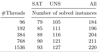
Table 8: Results from HordeSAT for the ap-plication benchmarks from the SAT Compe-tition 2016.

SAT UNS All

#Threads Number of solved instances

96 79 105 184

192 85 111 196

384 88 116 204

768 90 121 211

1536 93 127 220

process. In a massively-parallel setting, the clause databases of each solver thread contain more received than locally learned clauses. Thus, most clauses used in creating a proof have been strengthened by one solver.

Results for this experiment are given in Table 6. A clear performance improvement on unsatisfiable formulas can be observed. For example, the configuration on 768 solver threads can solve more unsatisfiable formulas than the configuration on 1536 threads and lazy clause exchange. Furthermore, the configuration on 1536 threads can solve 32 more unsatisfiable formulas than the VBS created from sequential solvers, and 8 more compared to the VBS made from parallel solvers.

4.2.4 Diversified Search

The final result we present uses the diversified search strategy discussed in Subsection3.4. As we considered this strategy to be stronger on satisfiable instances, we sought to balance to configuration to be also strong on unsatisfiable benchmarks. As suggested in [42], we slightly increased the LBD threshold for clauses to become permanent to 4. Some results for this setting are given in Table 7. Unfortunately we ran out of credits for our cluster at the time we ran these experiments, thus we can unfortunately only give results for up to 384 threads. Still, we consider them interesting. Compared to the setting with simple clause exchange presented in Table 4, the number of satisfiable instances solved is slightly increased, while the solver is significantly stronger on unsatisfiable instances. On 96 threads, this configuration solves 4 more satisfiable, and 13 more unsatisfiable formulas.

4.3

Discussion of Results

4.4

Comparison to Other Solvers

Unfortunately, there are only few papers which report the scaling behavior of solvers above 100 CPU cores. Here, we compare our implementation to two other solvers. The sources of HordeSAT [10] are publicly available. Thus, we could test its scaling behavior on the same hardware and benchmark set. It is noteworthy that the version of HordeSAT for which results are reported in the respective publication is based on Lingeling, we thus kept it as is rather than modifying it.

The results are given in Table 8. HordeSAT also scales well, and is slightly faster than our solver when run on satisfiable formulas. On the contrary, it is significantly weaker on unsatisfiable benchmarks. On 96 CPU cores, it solves 105 unsatisfiable formulas, compared to 114 which are solved by the configuration shown in Table6which strengthens learned clauses. When using more parallel hardware, this gap widens. On 1536 CPU cores, our solver can solve 13 instances more than HordeSAT. Even the “lazy” configuration with limited clause exchange can solve 7 more instances here. This is a clear hint that the clause exchange does pay of in creating resolution proofs.

The authors of [5] report results for the same benchmark set and configurations on 128 and 256 cores, but with a time limit of only 900 seconds. The report 177 solved instances on 128 cores (73 SAT, 104 UNSAT), 184 solved instances (75 SAT, 109 UNSAT) on 256 cores. This per-formance is comparable to our implementation, although our underlying solver is significantly older.

5

Conclusion & Future Work

We present a highly parallel SAT solver which scales well on a wide range of formulas despite the limits of resolution proofs as investigated in [36]. We discuss several implementation details of this portfolio solver which seem to be crucial for a parallel solver in general. In particular, since our solver performs well against others despite its use of quite basic solver threads.

We hope that both the implementation details as well as the results are interesting, especially as access to massively-parallel is still limited. Thus, we consider it important to exchange as many experimental results as possible.

Compared to sequential solvers, parallel solvers can be tuned by even more parameters. For example, importing received clauses very eagerly as in ManySAT may cause the solver to backtrack quite often in cases where many clauses are received. On the contrary, only importing them during restarts may lead to long intervals without clause import, and thus increase the amount of redundant work performed by the solver. Thus, we intend to investigate good import strategies.

On hard formulas, the size of the database for learned clauses may become quite large. It would be interesting to see if there is a good, parallel approach to compress this set of clauses in a stronger way than just applying subsumption checks and self-subsuming resolution on it.

Lastly, hard combinatorial problems seem to be more suited to parallel solvers which split the search space by guiding paths. It would be interesting to detect such formulas, and adapt the solver strategy during the solving process.

References

[2] Gene M. Amdahl. Validity of the single processor approach to achieving large scale computing capabilities. InProceedings of the April 18-20, 1967, Spring Joint Computer Conference, AFIPS ’67 (Spring), pages 483–485, New York, NY, USA, 1967. ACM.

[3] Christian Artigues, Emmanuel Hebrard, Valentin Mayer-Eichberger, Mohamed Siala, and Toby Walsh. SAT and hybrid models of the car sequencing problem. In Helmut Simonis, editor,

Integration of AI and OR Techniques in Constraint Programming - 11th International Conference, CPAIOR 2014, Cork, Ireland, May 19-23, 2014. Proceedings, volume 8451 ofLNCS, pages 268– 283. Springer, 2014.

[4] Gilles Audemard, Jean-Marie Lagniez, Bertrand Mazure, and Lakhdar Sais. On freezing and reac-tivating learnt clauses. In Karem A. Sakallah and Laurent Simon, editors,Theory and Applications of Satisfiability Testing - SAT 2011 - 14th International Conference, SAT 2011, Ann Arbor, MI, USA, June 19-22, 2011. Proceedings, volume 6695 of LNCS, pages 188–200. Springer, 2011. [5] Gilles Audemard, Jean-Marie Lagniez, Nicolas Szczepanski, and S´ebastien Tabary. A distributed

version of syrup. In Gaspers and Walsh [28], pages 215–232.

[6] Gilles Audemard and Laurent Simon. Predicting learnt clauses quality in modern SAT solvers. In Craig Boutilier, editor,IJCAI 2009, Proceedings of the 21st International Joint Conference on Artificial Intelligence, Pasadena, California, USA, July 11-17, 2009, pages 399–404, 2009. [7] Gilles Audemard and Laurent Simon. Refining restarts strategies for SAT and UNSAT. In Michela

Milano, editor,Principles and Practice of Constraint Programming - 18th International Confer-ence, CP 2012, Qu´ebec City, QC, Canada, October 8-12, 2012. Proceedings, volume 7514 ofLNCS, pages 118–126. Springer, 2012.

[8] Gilles Audemard and Laurent Simon. Lazy clause exchange policy for parallel SAT solvers. In Carsten Sinz and Uwe Egly, editors,Theory and Applications of Satisfiability Testing - SAT 2014 - 17th International Conference, Held as Part of the Vienna Summer of Logic, VSL 2014, Vienna, Austria, July 14-17, 2014. Proceedings, volume 8561 ofLNCS, pages 197–205. Springer, 2014. [9] Gilles Audemard and Laurent Simon. Glucose and syrup in the sat’16. Proceedings of SAT

Competition, pages 40–41, 2016.

[10] Tomas Balyo, Peter Sanders, and Carsten Sinz. Hordesat: A massively parallel portfolio SAT solver. In Heule and Weaver [34], pages 156–172.

[11] Max Bannach, Sebastian Berndt, and Thorsten Ehlers. Jdrasil: A modular library for computing tree decompositions. In Costas S. Iliopoulos, Solon P. Pissis, Simon J. Puglisi, and Rajeev Raman, editors,16th International Symposium on Experimental Algorithms, SEA 2017, June 21-23, 2017, London, UK, volume 75 of LIPIcs, pages 28:1–28:21. Schloss Dagstuhl - Leibniz-Zentrum fuer Informatik, 2017.

[12] Paul Beame, Henry A. Kautz, and Ashish Sabharwal. Understanding the power of clause learning. In Georg Gottlob and Toby Walsh, editors,IJCAI-03, Proc. 18th Int. Joint Conf. on Artificial Intelligence, Acapulco, Mexico, Aug. 9-15, 2003, pages 1194–1201. Morgan Kaufmann, 2003. [13] Jeremias Berg and Matti J¨arvisalo. Sat-based approaches to treewidth computation: An

evalu-ation. In26th IEEE International Conference on Tools with Artificial Intelligence, ICTAI 2014, Limassol, Cyprus, November 10-12, 2014 [1], pages 328–335.

[14] Armin Biere. Picosat essentials. JSAT, 4(2-4):75–97, 2008.

[15] Armin Biere. Splatz, lingeling, plingeling, treengeling, yalsat entering the sat competition 2016.

Proceedings of SAT Competition, pages 44–45, 2016.

[16] Armin Biere. Cadical, lingeling, plingeling, treengeling and yalsat entering the sat competition 2017. SAT COMPETITION 2017, page 14, 2017.

[17] Armin Biere, Alessandro Cimatti, Edmund M. Clarke, Ofer Strichman, and Yunshan Zhu. Bounded model checking. Advances in Computers, 58:117–148, 2003.

Proceedings, volume 8402 ofLecture Notes in Computer Science, pages 158–167. Springer, 2014. [19] Jukka Corander, Tomi Janhunen, Jussi Rintanen, Henrik J. Nyman, and Johan Pensar. Learning

chordal markov networks by constraint satisfaction. In Christopher J. C. Burges, L´eon Bottou, Zoubin Ghahramani, and Kilian Q. Weinberger, editors, Advances in Neural Information Pro-cessing Systems 26: 27th Annual Conference on Neural Information ProPro-cessing Systems 2013. Proceedings of a meeting held December 5-8, 2013, Lake Tahoe, Nevada, United States., pages 1349–1357, 2013.

[20] Martin Davis, George Logemann, and Donald Loveland. A machine program for theorem-proving.

Commun. ACM, 5(7):394–397, July 1962.

[21] Niklas E´en and Armin Biere. Effective preprocessing in SAT through variable and clause elim-ination. In Fahiem Bacchus and Toby Walsh, editors, Theory and Applications of Satisfiability Testing, 8th International Conference, SAT 2005, St. Andrews, UK, June 19-23, 2005, Proceed-ings, volume 3569 ofLNCS, pages 61–75. Springer, 2005.

[22] Niklas E´en, Alexander Legg, Nina Narodytska, and Leonid Ryzhyk. Sat-based strategy extraction in reachability games. In Blai Bonet and Sven Koenig, editors,Proceedings of the Twenty-Ninth AAAI Conference on Artificial Intelligence, January 25-30, 2015, Austin, Texas, USA., pages 3738–3745. AAAI Press, 2015.

[23] Niklas E´en and Niklas S¨orensson. An extensible sat-solver. In Enrico Giunchiglia and Armando Tacchella, editors,Theory and Applications of Satisfiability Testing, 6th International Conference, SAT 2003. Santa Margherita Ligure, Italy, May 5-8, 2003 Selected Revised Papers, volume 2919 ofLNCS, pages 502–518. Springer, 2003.

[24] Thorsten Ehlers and Mike M¨uller. New bounds on optimal sorting networks. In Arnold Beckmann, Victor Mitrana, and Mariya Ivanova Soskova, editors,Evolving Computability - 11th Conference on Computability in Europe, CiE 2015, Bucharest, Romania, June 29 - July 3, 2015. Proceedings, volume 9136 ofLNCS, pages 167–176. Springer, 2015.

[25] Thorsten Ehlers and Dirk Nowotka. Sequential and parallel glucose hacks. SAT COMPETITION 2016, page 39, 2016.

[26] Thorsten Ehlers, Dirk Nowotka, and Philipp Sieweck. Communication in massively-parallel SAT solving. In26th IEEE International Conference on Tools with Artificial Intelligence, ICTAI 2014, Limassol, Cyprus, November 10-12, 2014 [1], pages 709–716.

[27] Ludovic Le Frioux, Souheib Baarir, Julien Sopena, and Fabrice Kordon. Painless: A framework for parallel SAT solving. In Gaspers and Walsh [28], pages 233–250.

[28] Serge Gaspers and Toby Walsh, editors. Theory and Applications of Satisfiability Testing - SAT 2017 - 20th International Conference, Melbourne, VIC, Australia, August 28 - September 1, 2017, Proceedings, volume 10491 ofLecture Notes in Computer Science. Springer, 2017.

[29] Kilian Gebhardt and Norbert Manthey. Parallel variable elimination on CNF formulas. In Ingo J. Timm and Matthias Thimm, editors,KI 2013: Advances in Artificial Intelligence - 36th Annual German Conference on AI, Koblenz, Germany, September 16-20, 2013. Proceedings, volume 8077 ofLNCS, pages 61–73. Springer, 2013.

[30] John L. Gustafson. Reevaluating amdahl’s law. Commun. ACM, 31(5):532–533, May 1988. [31] Youssef Hamadi, Sa¨ıd Jabbour, and Lakhdar Sais. Manysat: a parallel SAT solver.JSAT, 6(4):245–

262, 2009.

[32] Youssef Hamadi and Christoph M. Wintersteiger. Seven challenges in parallel SAT solving. AI Magazine, 34(2):99–106, 2013.

[33] Marijn Heule, Oliver Kullmann, Siert Wieringa, and Armin Biere. Cube and conquer: Guiding CDCL SAT solvers by lookaheads. In Kerstin Eder, Jo˜ao Louren¸co, and Onn Shehory, editors,

Hardware and Software: Verification and Testing - 7th International Haifa Verification Conference, HVC 2011, Haifa, Israel, December 6-8, 2011, Revised Selected Papers, volume 7261 of LNCS, pages 50–65. Springer, 2011.

2015 - 18th International Conference, Austin, TX, USA, September 24-27, 2015, Proceedings, volume 9340 ofLNCS. Springer, 2015.

[35] Marijn J. H. Heule, Oliver Kullmann, and Victor W. Marek. Solving and verifying the boolean pythagorean triples problem via cube-and-conquer. In Nadia Creignou and Daniel Le Berre, edi-tors,Theory and Applications of Satisfiability Testing - SAT 2016 - 19th International Conference, Bordeaux, France, July 5-8, 2016, Proceedings, volume 9710 ofLNCS, pages 228–245. Springer, 2016.

[36] George Katsirelos, Ashish Sabharwal, Horst Samulowitz, and Laurent Simon. Resolution and parallelizability: Barriers to the efficient parallelization of SAT solvers. In Marie desJardins and Michael L. Littman, editors, Proceedings of the Twenty-Seventh AAAI Conference on Artificial Intelligence, July 14-18, 2013, Bellevue, Washington, USA.AAAI Press, 2013.

[37] Damien Ledoux. An interlocking safety proof applied to the french rail network. SAT COMPE-TITION 2016, page 73, 2016.

[38] Mao Luo, Chu-Min Li, Fan Xiao, Felip Many`a, and Zhipeng L¨u. An effective learnt clause mini-mization approach for CDCL SAT solvers. In Carles Sierra, editor,Proceedings of the Twenty-Sixth International Joint Conference on Artificial Intelligence, IJCAI 2017, Melbourne, Australia, Au-gust 19-25, 2017, pages 703–711. ijcai.org, 2017.

[39] Jo˜ao Marques-Silva and Jordi Planes. Algorithms for maximum satisfiability using unsatisfiable cores. In Donatella Sciuto, editor,Design, Automation and Test in Europe, DATE 2008, Munich, Germany, March 10-14, 2008, pages 408–413. ACM, 2008.

[40] Matthew W. Moskewicz, Conor F. Madigan, Ying Zhao, Lintao Zhang, and Sharad Malik. Chaff: Engineering an efficient SAT solver. In Proc. 38th Design Automation Conf., DAC 2001, Las Vegas, NV, USA, June 18-22, 2001, pages 530–535. ACM, 2001.

[41] Robert Nieuwenhuis, Albert Oliveras, and Cesare Tinelli. Solving SAT and SAT modulo theories: From an abstract davis–putnam–logemann–loveland procedure to dpll(T).J. ACM, 53(6):937–977, 2006.

[42] Chanseok Oh. Between SAT and UNSAT: the fundamental difference in CDCL SAT. In Heule and Weaver [34], pages 307–323.

[43] Olga Ohrimenko, Peter J. Stuckey, and Michael Codish. Propagation = lazy clause generation. In Christian Bessiere, editor,Principles and Practice of Constraint Programming - CP 2007, 13th International Conference, CP 2007, Providence, RI, USA, September 23-27, 2007, Proceedings, volume 4741 ofLNCS, pages 544–558. Springer, 2007.

[44] C´edric Piette, Youssef Hamadi, and Lakhdar Sais. Vivifying propositional clausal formulae. In Malik Ghallab, Constantine D. Spyropoulos, Nikos Fakotakis, and Nikolaos M. Avouris, editors,

ECAI 2008 - 18th European Conference on Artificial Intelligence, Patras, Greece, July 21-25, 2008, Proceedings, volume 178 ofFrontiers in Artificial Intelligence and Applications, pages 525–529. IOS Press, 2008.

[45] John Alan Robinson. A machine-oriented logic based on the resolution principle.J. ACM, 12(1):23– 41, 1965.

[46] Niklas S¨orensson and Armin Biere. Minimizing learned clauses. In Oliver Kullmann, editor,Theory and Applications of Satisfiability Testing - SAT 2009, 12th International Conference, SAT 2009, Swansea, UK, June 30 - July 3, 2009. Proceedings, volume 5584 ofLNCS, pages 237–243. Springer, 2009.

[47] G. S. Tseitin. Automation of Reasoning: 2: Classical Papers on Computational Logic 1967–1970, chapter On the Complexity of Derivation in Propositional Calculus, pages 466–483. Springer Berlin Heidelberg, 1983.