Int. J. IndustrialMathematics (ISSN 2008-5621)
Vol. 12, No. 1, 2020 Article ID IJIM-1235, 8 pages Research Article
Local Annihilation Method and Some Stiff Problems
A. Abdollahi ∗†, E. Babolian ‡
Received Date: 2018-10-03 Revised Date: 2019-02-16 Accepted Date: 2019-04-11
————————————————————————————————–
Abstract
In this article, a new scheme inspired from collocation method is presented for numerical solution of stiff initial-value problems and Fredholm integral equations of the first kind based on the derivatives of residual function. Then, the error analysis of this method is investigated by presenting an error bound. The efficiency of the new method is compared with the efficiency of the collocation method by presenting some stiff and ill-posed test problems. Numerical comparisons indicate that the presented method yields accurate approximations in many cases in which the collocation method is failed.
Keywords: Local annihilation method; Residual function; Stiff problems; Ill-posed problems.
—————————————————————————————————–
1
Introduction
T
hmethods are efficient techniques for numeri-e Galerkin, collocation and least squares cal solutions of most functional equations [7, 18, 19, 20]. However, obtaining an accurate solu-tion by these methods fails for ill-posed prob-lems [4, 13, 27]. In many recent numerical ap-proaches, some accurate approximations are ob-tained by modifying the previous methods [3, 4, 15, 21, 22, 1]. L-stable [26], composite Runge-Kutta [2, 12], finite volume approximation [14] and the approximations based on wavelet bases [5,8,17] are among the most successful methods for the numerical solutions of such stiff problems in recent years. In this article, the attempt is to show that some simple techniques can some-∗Corresponding author. [email protected], Tel:+98(914)1765221.†Department of Mathematics, Maragheh Branch, Is-lamic Azad University, Maragheh, Iran.
‡Department of Mathematical Sciences and Computer, Kharazmi University, Tehran, Iran.
times be efficient. therefore, it is tried to get an approximate solution by local annihilating the residual function and its derivatives. The pre-sented method has a simple structure, suitable error bound and significant numerical results. To describe this method, we consider the functional equation
Ax=f, (1.1) where A is a linear operator and f is a known function. Let{pj}∞j=0be a basis for solution space
of the Eq. (1.1). Then we may approximate the unknown solution x by
xn(t) = n ∑
j=0
ajpj(t). (1.2)
By substituting (1.2) into (1.1), we find that
n ∑
j=0
ajqj(s) =f(s) +rn(s), a≤s≤b, (1.3)
where
qj(s) = (Apj)(s), j = 0,· · ·, n,
and rn is the residual function. For determining
the unknown coefficients {aj}nj=0 by collocation
method(CM), we should solve the following linear system of equations [9,19]
rn(si) = 0 =⇒ n ∑
j=0
ajqj(si) =f(si),
i= 0,· · ·, n,
where the collocation points {si}ni=0 are chosen
arbitrarily from [a, b].
In ill-posed functional equations (for example, Fredholm integral equations of the first kind), the condition number of the coefficient matrix of the above system is greatly enlarged by increasing n. Therefore, any approximate solution of Eq. (1.1) is determined by very large error [7,10]. In the new method, the derivatives of the residual function rn have a main role in reducing the
ill-posedness of the problem and the approximate solutions are determined in the form of multi-rule functions. The presented error analysis and numerical examples show that this method is ef-ficient and applicable for numerical solution of many ill-posed and stiff functional equations.
2
Description of the method
2.1 The main idea
Suppose that the exact solution of the functional equation (1.1) is approximated by (1.2). Accord-ing to the Eq. (1.3), the residual function can be written as
rn(s) = n ∑
j=0
ajqj(s)−f(s), a≤s≤b. (2.4)
Let {si}mi=0 be arbitrary selected points from
[a, b]. Suppose that the residual function rn is
infinitely differentiable on the set {si}mi=0 ( it is
assumed that the left and right derivatives exist at the boundary points). To determine the ap-proximate solution of (1.1) in a neighborhood of si, i= 0,· · ·, m, we set
r(nk)(si) = 0, k= 0,· · ·, n, (2.5)
wherern(k) denoteskth derivative ofrn. It follows
then from (2.4) that (for fixed i)
n ∑
j=0
aijqj(k)(si) =f(k)(si), (2.6)
k= 0,· · ·, n i= 0,· · ·, m.
The index i in the coefficients {aij}nj=0 denotes
that the approximate solutionxn(t) is determined
in a neighborhood of si. We denote this solution
by xn,i(t). The matrix form of the linear system
of equations (2.6) is as follows.
Q(i)a(i)=F(i), i= 0,· · ·, m (2.7)
or, in the equivalent block matrix form
Q(0) 0 · · · 0 0 Q(1) · · · 0
..
. ... . .. ... 0 0 · · · Q(m)
a(0) a(1) .. . a(m)
= F(0) F(1) .. . F(m)
, where
Q(i) =
q0(si) q1(si) · · · qn(si)
q0′(si) q1′(si) · · · qn′(si)
..
. ... . .. ... q(0n)(si) q1(n)(si) · · · q(nn)(si)
,
a(i)=(ai0 ai1 · · · ain )T
,
,
F(i)=(f(si) f′(si) · · · f(n)(si) )T
,
fori= 0,· · ·, mand 0∈R(m+1)×(m+1) is the zero matrix.
By solving the above linear system, the approx-imate solution of the functional equation (1.1) around the point si is determined by
xn,i(t) = n ∑
j=0
aijpj(t), i= 0,· · ·, m. (2.8)
By setting
t0=s0, ti=
si−1+si
2 , i= 1,· · ·, m,
Table 1: Maximum absolute error,∥e∥∞, for the Example3.1.
ε= 10−3 ε= 10−5
n CM LAM CM LAM
1 7.7178e−03 8.8784e−02 7.7254e−05 8.9575e−04 2 9.9593e+ 00 1.5909e−03 9.9996e+ 00 1.6195e−07 3 9.8806e+ 00 4.2570e−05 9.9988e+ 00 4.3728e−11 4 9.7824e+ 00 1.5185e−06 9.9978e+ 00 1.5741e−14 5 9.6722e+ 00 6.7700e−08 9.9967e+ 00 7.0827e−18 6 9.5536e+ 00 3.6217e−09 9.9954e+ 00 3.8243e−21 7 9.4290e+ 00 2.2602e−10 9.9941e+ 00 2.4091e−24 8 9.2997e+ 00 1.6119e−11 9.9927e+ 00 1.7344e−27 9 9.1671e+ 00 1.2931e−12 9.9913e+ 00 1.4047e−30 10 9.0317e+ 00 1.1525e−13 9.9898e+ 00 1.2641e−33 11 8.8945e+ 00 1.1298e−14 9.9883e+ 00 1.2514e−36 12 8.7558e+ 00 1.2082e−15 9.9868e+ 00 1.3514e−39 13 8.6161e+ 00 1.3995e−16 9.9851e+ 00 1.5810e−42 14 8.4758e+ 00 1.7456e−17 9.9841e+ 00 1.9918e−45 15 8.3352e+ 00 2.3326e−18 9.9838e+ 00 2.6888e−48
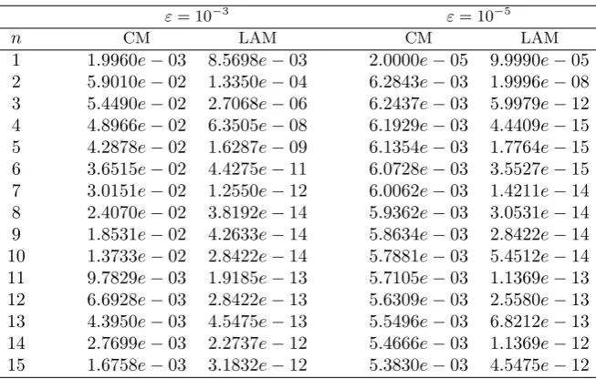
Table 2: Maximum absolute error,∥e∥∞, for the Example3.2.
ε= 10−3 ε= 10−5
n CM LAM CM LAM
1 1.9960e−03 8.5698e−03 2.0000e−05 9.9990e−05 2 5.9010e−02 1.3350e−04 6.2843e−03 1.9996e−08 3 5.4490e−02 2.7068e−06 6.2437e−03 5.9979e−12 4 4.8966e−02 6.3505e−08 6.1929e−03 4.4409e−15 5 4.2878e−02 1.6287e−09 6.1354e−03 1.7764e−15 6 3.6515e−02 4.4275e−11 6.0728e−03 3.5527e−15 7 3.0151e−02 1.2550e−12 6.0062e−03 1.4211e−14 8 2.4070e−02 3.8192e−14 5.9362e−03 3.0531e−14 9 1.8531e−02 4.2633e−14 5.8634e−03 2.8422e−14 10 1.3733e−02 2.8422e−14 5.7881e−03 5.4512e−14 11 9.7829e−03 1.9185e−13 5.7105e−03 1.1369e−13 12 6.6928e−03 2.8422e−13 5.6309e−03 2.5580e−13 13 4.3950e−03 4.5475e−13 5.5496e−03 6.8212e−13 14 2.7699e−03 2.2737e−12 5.4666e−03 1.1369e−12 15 1.6758e−03 3.1832e−12 5.3830e−03 4.5475e−12
, the approximate solution of Eq.(1.1) takes the piecewise function form
xn(t) =
∑n
j=0a0jpj(t) t0≤t < t1 ∑n
j=0a1jpj(t) t1≤t < t2
..
. ...
∑n
j=0amjpj(t) tm ≤t≤tm+1.
(2.9) We call this approach the local annihilation method(LAM).
2.2 Error analysis
In this section, the convergence of the local anni-hilation method is proved by presenting an error bound. Let {si}mi=0 be a set of partition points
in [a, b] and xn(t) given by (2.9) be the related
approximate solution. We define
|∆|= max
1≤i≤m|si−si−1|. (2.10)
and prove that the convergence order of the pre-sented method is O(n1!n).
Lemma 2.1 Let
max
0≤i≤m|r (k)
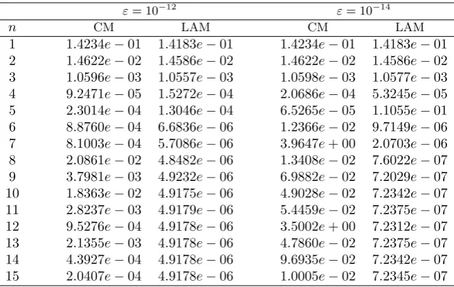
Table 3: Maximum absolute error,∥e∥∞, for the Example3.3A.
ε= 10−12 ε= 10−14
n CM LAM CM LAM
1 1.4234e−01 1.4183e−01 1.4234e−01 1.4183e−01 2 1.4622e−02 1.4586e−02 1.4622e−02 1.4586e−02 3 1.0596e−03 1.0557e−03 1.0598e−03 1.0577e−03 4 9.2471e−05 1.5272e−04 2.0686e−04 5.3245e−05 5 2.3014e−04 1.3046e−04 6.5265e−05 1.1055e−01 6 8.8760e−04 6.6836e−06 1.2366e−02 9.7149e−06 7 8.1003e−04 5.7086e−06 3.9647e+ 00 2.0703e−06 8 2.0861e−02 4.8482e−06 1.3408e−02 7.6022e−07 9 3.7981e−03 4.9232e−06 6.9882e−02 7.2029e−07 10 1.8363e−02 4.9175e−06 4.9028e−02 7.2342e−07 11 2.8237e−03 4.9179e−06 5.4459e−02 7.2375e−07 12 9.5276e−04 4.9178e−06 3.5002e+ 00 7.2312e−07 13 2.1355e−03 4.9178e−06 4.7860e−02 7.2375e−07 14 4.3927e−04 4.9178e−06 9.6935e−02 7.2342e−07 15 2.0407e−04 4.9178e−06 1.0005e−02 7.2345e−07
Table 4: Maximum absolute error,∥e∥∞, for the Example3.3B.
ε= 10−12 ε= 10−14
n CM LAM CM LAM
1 2.2327e−02 2.2327e−02 2.2327e−02 2.2327e−02 2 3.4053e−04 1.7924e−03 1.7414e−03 1.7916e−03 3 9.9720e−05 6.3374e−04 5.8595e−03 6.3851e−04 4 4.2923e−05 2.6353e−05 4.7434e−03 2.7155e−05 5 4.7167e−05 5.4294e−06 8.7616e−03 6.4914e−06 6 6.4304e−05 9.3344e−07 3.7614e−03 6.4517e−06 7 8.9088e−05 7.5238e−07 1.2446e−02 6.4519e−06 8 3.7391e−04 7.7152e−07 1.6332e−02 6.4520e−06 9 1.5598e−04 7.7213e−07 1.8612e−02 6.4520e−06 10 3.3079e−04 7.7207e−07 7.6010e−02 6.4520e−06 11 1.0750e−04 7.7207e−07 1.8536e−02 6.4520e−06 12 6.5696e−05 7.7207e−07 2.0952e−02 6.4520e−06 13 1.4975e−04 7.7207e−07 3.3348e−03 6.4520e−06 14 1.3171e−04 7.7207e−07 6.0423e−03 6.4520e−06 15 5.1317e−05 7.7207e−07 1.0364e−02 6.4520e−06
and |∆|<1.Then we have
|rn(s)|≤M(
1 (n+ 1)! +
1
(n+ 2)! +· · ·). f or all s∈[a, b]
Let s ∈ [a, b] be arbitrary. Then there exists a positive integer 0≤l≤m such that
|s−sl|= min
0≤i≤m|s−si|.
By using Taylor expansion ofrn(s)around sl, we have
rn(s) =rn(sl) +
(s−sl)1
1! r ′
n(sl) +· · ·+
(s−sl)n
n! r
(n) n (sl) +
(s−sl)n+1
(n+ 1)! r
(n+1)
n (sl) +· · ·. By the requirements (2.5) one gets
rn(s) =
(s−sl)n+1
(n+ 1)! r
(n+1) n (sl)+
(s−sl)n+2
(n+ 2)! r
(n+2)
n (sl) +· · ·. Therefore, the assumptions
|r(nk)(sl)|≤M, k=n+ 1, n+ 2,· · ·, and
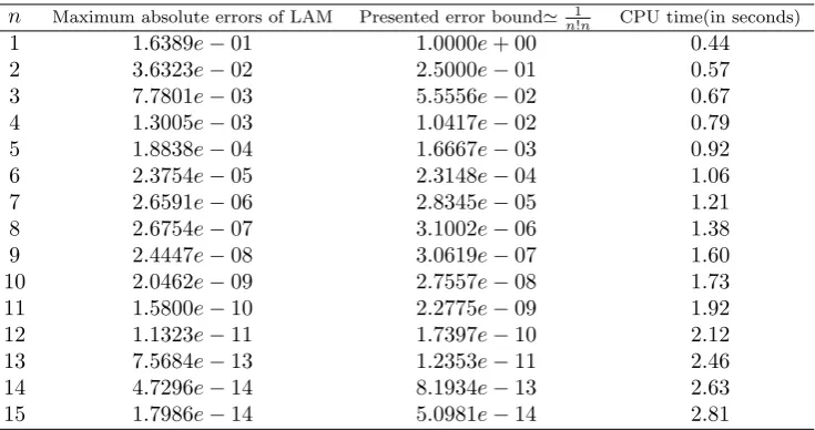
Table 5: Confirming the presented error bound and CPU time for the Example3.4.
n Maximum absolute errors of LAM Presented error bound≃n1!n CPU time(in seconds) 1 1.6389e−01 1.0000e+ 00 0.44 2 3.6323e−02 2.5000e−01 0.57 3 7.7801e−03 5.5556e−02 0.67 4 1.3005e−03 1.0417e−02 0.79 5 1.8838e−04 1.6667e−03 0.92 6 2.3754e−05 2.3148e−04 1.06 7 2.6591e−06 2.8345e−05 1.21 8 2.6754e−07 3.1002e−06 1.38 9 2.4447e−08 3.0619e−07 1.60 10 2.0462e−09 2.7557e−08 1.73 11 1.5800e−10 2.2775e−09 1.92 12 1.1323e−11 1.7397e−10 2.12 13 7.5684e−13 1.2353e−11 2.46 14 4.7296e−14 8.1934e−13 2.63 15 1.7986e−14 5.0981e−14 2.81
complete the proof.
Lemma 2.2 [25] For any positive integer n we have
e−
n ∑
k=0
1 k! <
1 n!n.
Corollary 2.1 By the assumptions of Lemma
2.1, for each positive integer n, we have
|rn(s)|≤
M
n!n, s∈[a, b]. Since
1 (n+ 1)! +
1
(n+ 2)! +· · ·=e−
n ∑
k=0
1 k!,
then by Lemmas 2.1 and 2.2, we have
|rn(s)|≤
M n!n, that is,
|rn(s)|=O(
1
n!n). (2.11) It should be mentioned that, the error bound in Corollary 2.1 may be violated by ill-posed prob-lems, since in this case the linear systems (2.7) usually have large condition numbers.
3
Test problems
In this section, we consider some stiff and ill-posed functional equations of the form (1.1) in order to compare accuracy of collocation method with our new local annihilation method.
Case 1:
In this case, we deal with the stiff initial-value problem [11].
(Ax)(s) =εx′(s) +a(s)x(s),
x(0) =x0, s∈[0, T].
These equations are characterized by the pres-ence of a small parameter as coefficient of the first-order derivative. These problems are stiff and ill-posed when ε→ 0 and have been treated numerically by using various approaches [13,24].
Case 2:
Let
(Ax)(s) =
∫ b
a
k(s, t)x(t)dt.
is presented by Tikhonov and Phillips [27,23] in-dependently. This method transforms the Fred-holm integral equation of the first kind
∫ b
a
k(s, t)x(t)dt=f(s), s∈[a, b],
to the following Fredholm integral equation of the second kind(regularized equation)
εxε(s) + ∫ b
a
k∗k(s, t)xε(t)dt= (3.12)
(k∗f)(s), s∈[a, b], where [10]
k∗k(s, t) =
∫ b
a
k(u, s)k(u, t)du,
(k∗f)(s) =
∫ b
a
k(u, s)f(u)du, s, t∈[a, b],
and ε is a small positive parameter called the regularization parameter. Also, Tikhonov and Phillips [16,23] showed that
lim
ε→0xε(s) =x(s)
By the above assumptions, we solve equation (3.12) by collocation and the new method. The presented numerical examples show that the new method is more accurate and stable than the col-location method.
Note
For computing the related integrals, we use a Gaussian quadrature rule of order 10 with 16 significant digits(by MATLAB R2013b) and max-imum precision is used in solving stiff problems. In the following tables the collocation method and the local annihilation method are denoted by CM and LAM respectively. The maximum absolute error ∥e∥∞ for the following examples is computed by ∥e∥∞= max|x(s) − xn(si)| in
collocation points. The basis functions are chosen as pj(t) =tj, j = 0,· · ·, n.
Example 3.1 Consider the initial value problem
εx′(s) +x(s) =g(s) +εg′(s),
x(0) = 10, s∈[0, T],
where g(s) = 10−(10 +s)exp(−s) and the exact solution is xε(s) = g(s) + 10exp(−sε). The prob-lem explains an initial layer of thickness O(ε) at x = 0 (see [13, 24] for more details). We solve this perturbed problem forε= 10−3and10−5with T = 1. For these values ofε, the errors of dynam-ical systems method(DSM), proposed in [24], are about 2.9 ×10⁻³ while our method shows more accurate results (see Table 1).
Example 3.2 Consider
εx′(s) + 1
1 +sx(s) =e −√s
ε( 1 1 +s−
√
ε),
x(0) = 1, s∈[0,1],
with the exact solution xε(s) = e−
s √
ε. The
nu-merical results are given in Table 2 for ε= 10−3
and 10−5.
Example 3.3 A:
∫ 1
0
estx(t)dt= e
s+1−1
s+ 1 , s∈[0,1].
B: ∫
π 6
0
cos(s−t)x(t)dt=
3sin(s) + (2π+ 3√3)cos(s)
24 , s∈[0, π 6].
The exact solutions are respectively es and cos(s). We solve the perturbed regularized forms of A and B for ε = 10−12 and 10−14 with the collocation and the new method. The error of ap-proximate solution for the equationA is of order O(10−5)by augmented Galerkin method [4], while our new method is more accurate than the aug-mented Galerkin method (see Table 3 and Table
4).
Example 3.4
x(s)− 1 2
∫ 1
0
(1 +s)e−stx(t)dt=
e−s+1 2(e
−(1+s)−1), s∈[0,1].
The exact solution is e−s. The numerical results and CPU time for local annihilation method(LAM) are shown in Table 5.
4
Conclusion
The numerical results show that the local anni-hilation method is often more accurate and more stable than the collocation method for the numer-ical solution of the presented stiff and ill-posed problems. Moreover, this new method can be considered as a new approach in solving many stiff engineering problems. It is also shown by examples 1-3 that this method can be used as an efficient method for solving problems where the collocation method fails. Finally, the numerical results of example 4 confirm the presented error bound of the well-posed problems.
Acknowledgement
The authors of this manuscript would like to thank Maragheh Branch, Islamic Azad University for its funding support and assistance through all aspects of this study. This manuscript is ex-tracted from the internal research project enti-tled: Local annihilation method for the numerical solution of some ill-posed problems.
References
[1] A. Abdollahi, E. Babolian, Theory of block-pulse functions in numerical solution of Fredholm integral equations of the second kind,Int. J. Industrial Mathematics8 (2016) 157-163.
[2] R. R. Ahmad, N. Yaacob, Third-order com-posite Runge-Kutta method for stiff prob-lems, International Journal of Computer Mathematics 82 (2006) 1221-1226.
[3] E. Babolian, A. Abdollahi, S. Shahmorad, Chain least squares method and ill-posed problems, Iranian Journal of Science & Technology 38 (2014) 123-132.
[4] E. Babolian, L. M. Delves, An augmented Galerkin method for first kind Fredholm equations,J. Inst. Maths. Applics 24 (1979) 157-174.
[5] E. Babolian, T. Lotfi, M. Paripour, Wavelet moment method for solving Fredholm in-tegral equations of the first kind, Applied Mathematics and Computation 186 (2007) 1467-1471.
[6] C. A. Balanis, Advanced Engineering Elec-tromagnetics, Wiley, New York, (1989).
[7] A. V. Bitsadze, Integral Equations of First Kind, World Scientific Publishing Co. Pte. Ltd., (1995).
[8] N. M. Bujurke, C. S. Salimath, S. C. Shi-ralashetti, Numerical solution of stiff sys-tems from nonlinear dynamics using single-term Haar wavelet series,Nonlinear Dynam-ics 51 (2008) 595-605.
[9] B. N. Datta, Numerical Linear Algebra and Applications Second Edition,SIAM, (2010).
[10] L. M. Delves, J. L. Mohamed, Computa-tional Methods for Integral Equations, Cam-bridge University Press, (1985).
[11] H. Ernst, W. Gerhard, Solving ordinary dif-ferential equations II: Stiff and difdif-ferential- differential-algebraic problems, Springer-Verlag, New York, (1996).
[12] B. Faleichik, I. Bondar, V. Byl, Generalized Picard iterations: A class of iterated Runge Kutta methods for stiff problems, Journal of Computational and Applied Mathematics
262 (2014) 37-50.
[13] P. A. Farrell, Uniform and optimal schemes for stiff initial value problems, Comput. Math. Applic. 13 (1987) 925-936.
two-dimensional curvilinear domain, Inter-national Journal of Computer Mathematics
93 (2015) 1787-1799.
[15] F. Goharee, E. Babolian, A. Abdollahi, Modified chain least squares method and some numerical results, Iranian Journal of Science & Technology 38 (2014) 91-99.
[16] C. W. Groetsch, The Theory of Tikhonov Regularization for Fredholm Equations of the First Kind, Research Notes in Mathe-matics, Boston MA, (1984).
[17] C. Hsiao, Numerical solution of stiff differ-ential equations via Haar wavelets, Interna-tional Journal of Computer Mathematics 82 (2006) 1117-1123.
[18] R. Kress, Linear Integral Equations,
Springer-Verlag, (1999).
[19] R. Kress, Numerical Analysis, Springer-Verlag, New York, (1998).
[20] H. N. Mhaskar, D. V. Pai, Fundamentals of Approximation Theory, DAlpha Science In-ternational Ltd.(2000).
[21] P. Novati, A class of explicit one-step meth-ods of order two for stiff problems,Journal of Numerical Mathematics 13 (2005) 219-236.
[22] R. I. Okuonghae, M. N. O. Ikhile, A class of hybrid linear multistep methods with A-stability properties for stiff IVPs in ODEs,
Journal of Numerical Mathematics21 (2013) 157-172.
[23] D. L. Phillips, A technique for the numerical solution of certain integral equations of the first kind, J. Ass. Comput. Mach. 9 (1962) 84-96.
[24] J. I. Ramos, Linearization techniques for singularity-perturbed initial-value problems of ordinary differential equations, Applied Mathematics and Computation 163 (2005) 1143-1163.
[25] W. Rudin, Principles of Mathematical Anal-ysis 3nd ed., McGraw-Hill, New York, (1976).
[26] R. E. Scraton, Some L-stable methods for stiff differential equations, International Journal of Computer Mathematics 9 (2007) 81-87.
[27] A. N. Tikhonov, A. Goncharsky, V. V. Stepanov, A. G. Yagola, Numerical Methods for the Solution of Ill-Posed Problems Dor-drecht,Boston, (1995).
Ali Abdollahi is Assistant profes-sor at the Department of Math-ematics, Maragheh Branch, Is-lamic Azad University, Maragheh, Iran. His research interests in-clude numerical solution of func-tional Equations, Numerical lin-ear algebra, Mathematical education, Numerical analysis and Integral Equations.