Vol. 5, No. 2, 2013 Article ID IJIM-00391, 11 pages Research Article
A study on Degasperis - Procesi equation by iterative methods
Sh. S. Behzadi∗ †
————————————————————————————————– Abstract
The Degasperis-Procesi equation can be derived as a member of a oneparameter family of asymptotic shallow water approximations to the Euler equations with the same asymptotic accuracy as that of the Camassa- Holm equation. In this paper, the Degasperis-Procesi equation is solved by using the Adomian’s decomposition method , modified Adomian’s decomposition method , variational iteration method , modified variational iteration method, homotopy perturbation method, modified homotopy perturbation method and homotopy analysis method. The existence and uniqueness of the solution and convergence of the proposed methods are proved in details. Finally an example shows the accuracy of these methods.
Keywords: Degasperis-Procesi equation; Adomian decomposition method (ADM); Modified Adomian decomposition method (MADM); Variational iteration method (VIM); Modified variational iteration method (MVIM); Homotopy perturbation method (HPM); Modified homotopy perturbation method (MHPM); Homotopy analysis method (HAM).
—————————————————————————————————–
1
Introduction
I
tnamic problems in physics and other fieldshas been shown that many important dy-are usually characterized by nonlinear evolution equations which are often called governing equa-tions [3, 42, 36, 27]. To understand the physical mechanism of these problems one has to study the solutions to the associated governing equations. Searching for the exact solutions of the nonlin-ear physical models has been a major concern for both mathematicians and physicists since they can provide much physical information and more insight into the physical aspects of the problems and thus maybe lead to further applications. Re-cently, some mathematician have studied the nu-merical solution of the Degasperis-Procesi equa-tion by numerical method [28,21,12,29,32,20].∗Corresponding author. shadan [email protected] †Department of Mathematics, Qazvin Branch, Islamic Azad University, Qazvin, Iran.
In this work, we develope the ADM, MADM, VIM, MVIM, HPM, MHPM and HAM to solve this equation as follows [28,21,29,32,20]:
ut−uxx =uuxxx+ 3uxuxx−4uux. (1.1)
With the initial condition:
u(x,0) =g(x). (1.2)
The paper is organized as follows. In Section 2, the mentioned iterative methods are introduced for solving Eq.(1.1). In Section 3 we prove the existence , uniqueness of the solution and convergence of the proposed methods. Finally, the numerical example is shown in Section 4. In order to obtain an approximate solution of Eq.(1.1), let us integrate one time Eq.(1.1) with respect to tusing the initial condition we obtain,
u(x, t) =g(x)
+
∫ t
0
F1(u(x, τ) dτ+
∫ t
0
F2(u(x, τ)) dτ
+ 3
∫ t
0
F3(u(x, τ))dτ
−4
∫ t
0
F4(u(x, τ)) dτ,
(1.3)
where,
F1(u(x, t)) =uxx(x, t),
F2(u(x, t)) =u(x, t)uxxx(x, t),
F3(u(x, t)) =ux(x, t)uxx(x, t),
F4(u(x, t)) =u(x, t)ux(x, t).
In Eq.(1.3), we assume g(x) is bounded for allx
in J = [0, T](T ∈ R). The terms F1(u(x, t)) ,
F2(u(x, t)), F3(u(x, t)) and F4(u(x, t)) are
Lips-chitz continuous with | F1(u)−F1(u∗) |≤ L1 |
u −u∗ | , | F2(u) −F2(u∗) |≤ L2 | u−u∗ |,
| F3(u)−F3(u∗) |≤ L3 | u−u∗ | and | F4(u)−
F4(u∗)|≤L4 |u−u∗|.
2
The iterative methods
2.1 Description of the MADM and ADM
The Adomian decomposition method is applied to the following general nonlinear equation
Lu+Ru+N u=f, (2.4)
where u(x, t) is the unknown function, L is the highest order derivative operator which is as-sumed to be easily invertible, R is a linear dif-ferential operator of order less than L, N u rep-resents the nonlinear terms, and f is the source term. Applying the inverse operatorL−1 to both sides of Eq.(2.4), and using the given conditions we obtain
u(x, t) =z(x)−L−1(Ru)−L−1(N u), (2.5)
where the functionz(x) represents the terms aris-ing from integrataris-ing the source termf. The non-linear operator N u=G1(u) is decomposed as
G1(u) =
∞
∑
n=0
An, (2.6)
where An, n ≥ 0 are the Adomian polynomials
determined formally as follows:
An=
1
n![
dn dλn[N(
∞
∑
i=0
λiui)]]λ=0. (2.7)
The first Adomian polynomials (introduced in [7,
14,34] ) are:
A0=G1(u0),
A1=u1G′1(u0),
A2=u2G′1(u0) +
1 2!u
2
1G′′1(u0), (2.8)
A3=u3G′1(u0) +u1u2G′′1(u0) +
1 3!u
3
1G′′′1 (u0), ...
2.1.1 Adomian decomposition method
The standard decomposition technique represents the solution ofu(x, t) in Eq.(2.4) as the following series,
u(x, t) =
∞
∑
i=0
ui(x, t), (2.9)
where, the components u0, u1, . . . which can be
determined recursively
u0(x, t) =g(x),
u1(x, t) =
∫ t
0
A0(x, t) dt+
∫ t
0
B0(x, t) dt
+3
∫ t
0
Z0(x, t) dt−4
∫ t
0
K0(x, t)dt,
.. .
un+1(x, t) =
∫ t
0
An(x, t) dt+
∫ t
0
Bn(x, t) dt+
3
∫ t
0
Zn(x, t) dt−4
∫ t
0
Kn(x, t) dt,
n≥0. (2.10)
Substituting Eq.(2.8) into Eq.(2.10) leads to the determination of the components ofu.
2.1.2 The modified Adomian decomposi-tion method
The modified decomposition method was intro-duced by Wazwaz [35]. The modified forms was established on the assumption that the function
g(x) can be divided into two parts, namely g1(x)
and g2(x). Under this assumption we set
Accordingly, a slight variation was proposed only on the componentsu0andu1. The suggestion was
that only the part g1 be assigned to the zeroth
component u0, whereas the remaining part g2 be
combined with the other terms given in Eq.(2.11) to define u1. Consequently, the modified
recur-sive relation
u0=g1(x),
u1=g2(x)−L−1(Ru0)−L−1(A0), (2.12)
.. .
un+1=−L−1(Run)−L−1(An), n≥1,
was developed. To obtain the approximation so-lution of Eq.(1.1), according to the MADM, we can write the iterative formula Eq.(2.12) as fol-lows:
u0 =g1(x),
u1 =g2(x) +
∫t
0A0(x, t) dt+
∫t
0B0(x, t)dt
+ 3∫0tZ0(x, t) dt−4
∫t
0K0(x, t) dt,
.. .
un+1=
∫t
0An(x, t) dt+
∫t
0Bn(x, t) dt
+ 3∫0tZn(x, t) dt−4
∫t
0Kn(x, t)dt, n≥1.
(2.13) The operators Fi(u(x, t)) (i = 1,2,3,4) are
usu-ally represented by the infinite series of the Ado-mian polynomials as follows:
F1(u) =
∞
∑
i=0
Ai,
F2(u) =
∞
∑
i=0
Bi,
F3(u) =
∞
∑
i=0
Zi,
F4(u) =
∞
∑
i=0
Ki.
where Ai, Bi,Zi and Ki are the Adomian
poly-nomials. Also, we can use the following formula for the Adomian polynomials [13]:
An=F1(sn)−∑ni=0−1Ai,
Bn=F2(sn)−
∑n−1
i=0 Bi,
Zn=F3(sn)−
∑n−1
i=0 Zi,
Kn=F4(sn)−
∑n−1
i=0 Ki.
(2.14)
Wheresn=
∑n
i=0ui(x, t) is the partial sum.
2.2 Description of the VIM and MVIM
In the VIM [1, 2, 15, 22, 23, 24, 25, 38], it has been considered the following nonlinear differen-tial equation:
Lu+N u=g, (2.15)
where L is a linear operator, N is a nonlinear operator and g is a known analytical function. In this case, the functionsun may be determined
recursively by
un+1(x, t) =un(x, t)+
∫ t
0
λ(x, τ){L(un(x, τ))+N(un(x, τ))−g(x, τ)}dτ,
(2.16)
n≥0,
where λ is a general Lagrange multiplier which can be computed using the variational theory. Here the function un(x, τ) is a restricted
varia-tions which means δun = 0. Therefore, we first
determine the Lagrange multiplier λthat will be identified optimally via integration by parts. The successive approximation un(x, t), n ≥ 0 of the
solution u(x, t) will be readily obtained upon us-ing the obtained Lagrange multiplier and by usus-ing any selective functionu0. The zeroth
approxima-tionu0may be selected any function that just
sat-isfies at least the initial and boundary conditions. With λ determined, then several approximation
un(x, t),n≥0 follow immediately. Consequently,
the exact solution may be obtained by using
u(x, t) = lim
n→∞un(x, t). (2.17)
The VIM has been shown to solve effectively, eas-ily and accurately a large class of nonlinear prob-lems with approximations converge rapidly to ac-curate solutions. To obtain the approximation solution of Eq.(1.1), according to the VIM, we can write iteration Eq.(2.16) as follows:
un+1(x, t) =un(x, t) +Lt−1(λ[un(x, t)−g(x)−
∫t
0F1(un(x, t))dt−
∫t
0F2(un(x, t))dt−
3∫0tF3(un(x, t))dt+ 4
∫t
0F4(un(x, t))dt]),
n≥0.
Where,
L−t1(.) =
∫ t
0
(.) dτ.
To find the optimalλ, we proceed as
δun+1(x, t) =δun(x, t) +δLt−1(λ[un(x, t)−g(x)
−∫t
0F1(un(x, t))dt−
∫t
0F2(un(x, t))dt−
3∫0tF3(un(x, t))dt+ 4
∫t
0 F4(un(x, t))dt]).
(2.19) From Eq.(2.19), the stationary conditions can be obtained as follows: λ′ = 0 and 1 +λ= 0. There-fore, the Lagrange multipliers can be identified as λ=−1 and by substituting in Eq.(2.18), the following iteration formula is obtained.
u0(x, t) =g(x),
un+1(x, t) =un(x, t)−Lt−1(un(x, t)−g(x)
−∫t
0F1(un(x, t))dt−
∫t
0F2(un(x, t))dt−3
∫t
0 F3(un(x, t))dt+ 4
∫t
0F4(un(x, t))dt), n≥0.
(2.20) To obtain the approximation solution of Eq.(1.1), based on the MVIM [4, 5, 37], we can write the following iteration formula:
u0(x, t) =g(x),
un+1(x, t) =un(x, t)−
L−t1(−∫0tF1(un(x, t)−u(x, t)) dt−
∫t
0F2(un(x, t)−u(x, t)) dt−
3∫0tF3(un(x, t)−u(x, t)) dt
+4∫0tF4(un(x, t)−u(x, t))dt), n≥0.
(2.21)
Eq.(2.20) and Eq.(2.21) will enable us to de-termine the components un(x, t) recursively for
n≥0.
2.3 Description of the HAM
Consider
N[u] = 0,
where N is a nonlinear operator, u(x, t) is an unknown function and x is an independent vari-able. let u0(x, t) denote an initial guess of the
exact solution u(x, t), h̸= 0 an auxiliary param-eter, H1(x, t) ̸= 0 an auxiliary function, and L
an auxiliary linear operator with the property
L[s(x, t)] = 0 when s(x, t) = 0. Then using
q ∈ [0,1] as an embedding parameter, we con-struct a homotopy as follows:
(1−q)L[ϕ(x, t;q)−u0(x, t)]
−qhH1(x, t)N[ϕ(x, t;q)] =
ˆ
H[ϕ(x, t;q);u0(x, t), H1(x, t), h, q]. (2.22)
It should be emphasized that we have great free-dom to choose the initial guessu0(x, t), the
aux-iliary linear operator L, the non-zero auxiliary parameterh, and the auxiliary functionH1(x, t).
Enforcing the homotopy Eq.(2.22) to be zero, i.e.,
ˆ
H1[ϕ(x, t;q);u0(x, t), H1(x, t), h, q] = 0, (2.23)
we have the so-called zero-order deformation equation
(1−q)L[ϕ(x, t;q)−u0(x, t)] =
qhH1(x, t)N[ϕ(x, t;q)]. (2.24)
When q = 0, the zero-order deformation Eq.(2.24) becomes
ϕ(x; 0) =u0(x, t), (2.25)
and whenq= 1, sinceh̸= 0 andH1(x, t)̸= 0, the
zero-order deformation Eq.(2.24) is equivalent to
ϕ(x, t; 1) =u(x, t). (2.26)
Thus, according to Eq.(2.25) and Eq.(2.26), as the embedding parameterqincreases from 0 to 1,
ϕ(x, t;q) varies continuously from the initial ap-proximation u0(x, t) to the exact solutionu(x, t).
Such a kind of continuous variation is called de-formation in homotopy [8,11,16,30,31]. Due to Taylor’s theorem, ϕ(x, t;q) can be expanded in a power series ofq as follows
ϕ(x, t;q) =u0(x, t) +
∞
∑
m=1
um(x, t)qm, (2.27)
where,
um(x, t) =
1
m!
∂mϕ(x, t;q)
∂qm |q=0 .
Let the initial guess u0(x, t), the auxiliary
lin-ear parameter L, the nonzero auxiliary parame-terhand the auxiliary functionH1(x, t) be
ϕ(x, t;q) converges atq= 1, then, we have under these assumptions the solution series
u(x, t) =ϕ(x, t; 1) =u0(x, t) +
∞
∑
m=1
um(x, t).
(2.28) From Eq.(2.27), we can write Eq.(2.24) as follows
(1−q)L[ϕ(x, t, q)−u0(x, t)] =
(1−q)L[∑∞m=1um(x, t) qm] =
q h H1(x, t)N[ϕ(x, t, q)]⇒
L[∑∞m=1um(x, t) qm]−q L[
∑∞
m=1um(x, t)qm]
=q h H1(x, t)N[ϕ(x, t, q)]
(2.29) By differentiating Eq.(2.29)mtimes with respect toq, we obtain
{L[∑∞m=1um(x, t) qm]−
q L[∑∞m=1um(x, t)qm]}(m)=
{q h H1(x, t)N[ϕ(x, t, q)]}(m) =
m! L[um(x, t)−um−1(x, t)] =
h H1(x, t) m ∂
m−1N[ϕ(x,t;q)]
∂qm−1 |q=0 .
Therefore,
L[um(x, t)−χmum−1(x, t)] =
hH1(x, t)ℜm(um−1(x, t)),
(2.30)
where,
ℜm(um−1(x, t)) =
1 (m−1)!
∂m−1N[ϕ(x, t;q)]
∂qm−1 |q=0, (2.31)
and
χm =
{
0, m≤1 1, m >1
Note that the high-order deformation Eq.(3.7) is governing the linear operator L, and the termℜm(um−1(x, t)) can be expressed simply by
Eq.(2.31) for any nonlinear operator N. To ob-tain the approximation solution of Eq.(1.1),
ac-cording to HAM, let
N[u(x, t)] =u(x, t)−g(x)−∫0tF1(u(x, t))dt−
∫t
0F2(u(x, t))dt−3
∫t
0u(x, t) dt
+4∫0tF4(u(x, t)) dt−3
∫t
0u(x, t) dt,
so,
ℜm(um−1(x, t)) =um−1(x, t)−g(x)−
∫t
0F1(um−1(x, t))dt−
∫t
0F2(um−1(x, t))dt−
3∫0tF3(um−1(x, t))dt+ 4
∫t
0F4(um−1(x, t))dt.
(2.32) Substituting Eq.(2.32) into Eq.(3.7)
L[um(x, t)−χmum−1(x, t)] =
hH1(x, t)[um−1(x, t)−g(x)−
∫t
0F1(um−1(x, t))dt−
∫t
0F2(um−1(x, t))dt−
3∫0tF3(um−1(x, t))dt+ 4
∫t
0F4(um−1(x, t))dt.
+(1−χm)g(x)(x)].
(2.33) We take an initial guess u0(x, t) =g(x), an
aux-iliary linear operator Lu = u, a nonzero auxil-iary parameter h = −1, and auxiliary function
H1(x, t) = 1. This is substituted into Eq.(2.33)
to give the recurrence relation
u0(x, t) =g(x),
un+1(x, t) =
∫t
0F1(un(x, t))dt+
∫t
0F2(un(x, t))dt+ 3
∫t
0F3(un(x, t))dt
−4∫0tF4(un(x, t))dt, n≥0.
(2.34)
Therefore, the solution u(x, t) becomes
u(x, t) =∑∞n=0un(x, t) =g(x)
+∑∞n=1( ∫0tF1(un(x, t))dt+
∫t
0F2(un(x, t))dt
+3∫0tun(x, t) dt−4
∫t
0F4(un(x, t))dt.
(2.35) Which is the method of successive approxima-tions. If
|un(x, t)|<1,
2.4 Description of the HPM and MHPM
To explain HPM [9, 10, 18, 33, 39, 40, 41] , we consider the following general nonlinear differen-tial equation:
Lu+N u=f(u), (2.36)
with initial conditions
u(x,0) =f(x).
According to HPM, we construct a homotopy which satisfies the following relation
H(u, p) =Lu−Lv0+p Lv0+p[N u−f(u)] = 0,
(2.37) where p ∈[0,1] is an embedding parameter and
v0 is an arbitrary initial approximation satisfying
the given initial conditions. In HPM, the solution of Eq.(2.37) is expressed as
u(x, t) =u0(x, t) +p u1(x, t) +p2 u2(x, t) +...
(2.38) Hence the approximate solution of Eq.(2.36) can be expressed as a series of the power of p, i.e.
u= lim
p→1u=u0+u1+u2+...
where,
u0(x, t) =g(x),
.. .
um(x, t) =
∑m−1
k=0
∫t
0F1(um−k−1(x, t)) dt+
∫t
0F2(um−k−1(x, t))dt+ 3
∫t
0F3(um−k−1(x, t))dt
−4∫0tF4(um−k−1(x, t)) dt, m≥1.
(2.39) To explain MHPM [6, 17, 26], we consider Eq.(1.1) as
L(u) =u(x, t)−g(x)−∫0tF1(um−k−1(x, t))dt−
∫t
0F2(um−k−1(x, t))dt−3
∫t
0F3(um−k−1(x, t))dt
+4∫0tF4(um−k−1(x, t)) dt.
Where F1(u(x, t)) = g1(x)h1(t), F2(u(x, t)) =
g2(x)h2(t), F3(u(x, t)) = g3(x)h3(t) and
F4(u(x, t)) = g4(x)h4(t). We can define
homo-topyH(u, p, m) by
H(u,0, m) =f(u), H(u,1, m) =L(u),
where, m is an unknown real number and
f(u(x, t)) =u(x, t)−z(x, t).
Typically we may choose a convex homotopy by
H(u, p, m) = (1−p)f(u) +p L(u)
+p(1−p)[m(g1(x) +g2(x) +g3(x)) +g4(x)] = 0,
(2.40) 0≤p≤1.
Where m is called the accelerating parameters, and for m = 0 we define H(u, p,0) = H(u, p),
which is the standard HPM. The convex homo-topy Eq.(2.40) continuously trace an implicity defined curve from a starting point H(u(x, t)−
f(u),0, m) to a solution functionH(u(x, t),1, m).
The embedding parameter p monotonically in-crease from 0 to 1 as trivial problem f(u) = 0 is continuously deformed to original problem
L(u) = 0. The MHPM uses the homotopy pa-rameterp as an expanding parameter to obtain
v=
∞
∑
n=0
pnun, (2.41)
when p → 1, Eq.(2.37) corresponds to the origi-nal one and Eq.(2.41) becomes the approximate solution of Eq.(1.1), i.e.,
u= lim
p→1v=
∞
∑
m=0
um.
Where,
u0(x, t) =g(x),
u1(x, t) =
∫t
0F1(u0(x, t))dt+
∫t
0F2(u0(x, t)) dt
+3∫0tF3(u0(x, t))dt
−m(g1(x) +g2(x) +g3(x) +g4(x)),
u2(x, t) =
∫t
0F1(u1(x, t))dt+
∫t
0F2(u1(x, t)) dt
+3∫0tF3(u1(x, t))dt−4
∫t
0F4(um−k−1(x, t)) dt
+m(g1(x) +g2(x) +g3(x) +g4(x)),
.. .
um(x, t) =
∑m−1
k=0
∫t
0F1(um−k−1(x, t))dt+
∫t
0 F2(um−k−1(x, t))dt+ 3
∫t
0F3(um−k−1(x, t))dt
−4∫0tF4(um−k−1(x, t))dt, m≥3.
3
Existence and convergency of
iterative methods
We set,
α1:=T(L1+L2+ 3L3+ 4L4),
β1 := 1−T(1−α1), γ1 := 1−T α1.
Theorem 3.1 Let 0< α1 <1, then
Degasperis-Procesi Eq.(1.1), has a unique solution.
Proof. Let u and u∗ be two different solutions of Eq.(1.3) then
|u−u∗ |=|∫0t[F1(u(x, t))−F1(u∗(x, t))] dt
+∫0t[F2(u(x, t))−F2(u∗(x, t))] dt
+3∫0t[F3(u(x, t))−F3(u∗(x, t))] dt−
4∫0t[F4(u(x, t))−F4(u∗(x, t))] dt|
≤∫t
0 |F1(u(x, t))−F1(u∗(x, t))| dt+
∫t
0 |F2(u(x, t))−F2(u∗(x, t))| dt+
∫t
0 |F3(u(x, t))−F3(u∗(x, t))| dt+
4∫0t|F4(u(x, t))−F4(u∗(x, t))| dt≤
T(L1+L2+ 3L3+ 4L4)|u−u∗|
=α1 |u−u∗ |.
From which we get (1−α1) |u−u∗ |≤0. Since
0 < α1 < 1, then |u−u∗ |= 0. Implies u =u∗
and completes the proof. 2
Theorem 3.2 The series solution u(x, t) =
∑∞
i=0ui(x, t) of Eq.(1.1) using MADM
conver-gence when 0 < α1 < 1, | u1(x, t) |< ∞.
Proof. Denote as (C[J],∥.∥) the Banach space of all continuous functions on J with the norm
∥ g(t) ∥= max | g(t) |, for all t in J. Define the sequence of partial sumssn, letsnandsm be
arbitrary partial sums with n ≥ m. We are go-ing to prove thatsn is a Cauchy sequence in this
Banach space:
∥sn−sm∥=max∀t∈J |sn−sm |=
max∀t∈J |
∑n
i=m+1ui(x, t)|=
max∀t∈J |
∫t
0(
∑n−1
i=mAi) dt+
∫t
0(
∑n−1
i=mBi)dt+
3∫0t(∑in=−m1 Zi) dt−4
∫t
0(
∑n−1
i=mKi) dt|.
From [13], we have
∑n−1
i=mAi=F1(sn−1)−F1(sm−1),
∑n−1
i=mBi =F2(sn−1)−F2(sm−1),
∑n−1
i=mZi=F3(sn−1)−F3(sm−1),
∑n−1
i=mKi =F4(sn−1)−F4(sm−1).
So,
∥sn−sm ∥=
max∀t∈J |
∫t
0[F1(sn−1)−F1(sm−1)]dt+
∫t
0[F2(sn−1)−F2(sm−1)]dt+
3∫0t[F3(sn−1)−(F3(sm−1)] dt−
4∫0t[F4(sn−1)−(F4(sm−1)] dt|≤
∫t
0 |F1(sn−1)−F1(sm−1)| dt+
∫t
0 |F2(sn−1)−F2(sm−1)| dt
+3∫0t|F3(sn−1)−F3(sm−1)| dt+
4∫0t|F4(sn−1)−F4(sm−1)| dt≤α1 ∥sn−sm ∥.
Let n=m+ 1, then
∥sn−sm∥≤α1 ∥sm−sm−1 ∥≤
α21 ∥sm−1−sm−2 ∥≤...≤α1m∥s1−s0 ∥.
From the triangle inquality we have
∥sn−sm ∥≤∥sm+1−sm∥
+∥sm+2−sm+1 ∥+...+∥sn−sn−1 ∥
≤[αm1 +α1m+1+...+α1n−m−1]∥s1−s0 ∥
≤αm1 [1 +α1+α21+...+αn1−m−1]∥s1−s0∥≤
αm1 [1−α
n−m
1
1−α1 ]∥u1(x, t)∥.
Since 0< α1 <1, we have (1−αn1−m)<1, then
∥sn−sm∥≤
αm1
1−α1
max∀t∈J |u1(x, t)|. (3.43)
But | u1(x, t) |< ∞ , so, as m → ∞, then
∥sn−sm ∥→0. We conclude thatsnis a Cauchy
Theorem 3.3 The maximum absolute trunca-tion error of the series solutrunca-tion u(x, t) =
∑∞
i=0ui(x, t) to Eq.(1.1) by using MADM is
esti-mated to be
max|u(x, t)−
m
∑
i=0
ui(x, t)|≤
kα1m
1−α1
. (3.44)
Proof. From inequality Eq.(3.43), when n → ∞, then sn→u and
max|u1(x, t)|≤T(max∀t∈J |F1(u0(x, t))|+
max∀t∈J |F2(u0(x, t))|+
3max∀t∈J |F3(u0(x, t))|+
4max∀t∈J |F4(u0(x, t))|).
Therefore,
∥u(x, t)−sm∥≤ α
m
1
1−α1T(max∀t∈J |F1(u0(x, t))|
+max∀t∈J |F2(u0(x, t))|+
3max∀t∈J |F3(u0(x, t))|+
4max∀t∈J |F4(u0(x, t))|).
Finally the maximum absolute truncation error in the intervalJ is obtained by Eq.(3.44).
Theorem 3.4 The solution un(x, t) obtained
from the relation Eq.(2.20) using VIM converges to the exact solution of the Eq.(1.1) when 0 < α1<1 and 0< β1 <1.
Proof.
un+1(x, t) =un(x, t)−Lt−1([un(x, t)−g(x)−
∫t
0 F1(un(x, t))dt−
∫t
0F2(un(x, t))dt
−3∫0tF3(un(x, t))dt+ 4
∫t
0F4(un(x, t))dt.])
(3.45)
u(x, t) =u(x, t)−Lt−1([u(x, t)−g(x)−
∫t
0 F1(u(x, t))dt−
∫t
0F2(u(x, t))dt
−3∫0tF3(u(x, t)) dt+ 4
∫t
0F4(u(x, t))dt.])
(3.46)
By subtracting relation Eq.(3.45) from Eq.(3.46),
un+1(x, t)−u(x, t) =un(x, t)−u(x, t)−
L−t1(un(x, t)−u(x, t)
∫t
0[F1(un(x, t))−
F1(u(x, t))]dt−
∫t
0[F2(un(x, t))−F2(u(x, t))] dt−
3∫0t[F3(un(x, t))−F3(u(x, t))] dt+
4∫0t[F4(un(x, t))−F4(u(x, t))] dt),
if we set, en+1(x, t) = un+1(x, t) − un(x, t),
en(x, t) = un(x, t)−u(x, t),| en(x, t∗) |= maxt |
en(x, t) | then since en is a decreasing function
with respect to t from the mean value theorem we can write,
en+1(x, t) =en(x, t) +L−t1(−en(x, t)−
∫t
0[F1(un(x, t))−F1(u(x, t))] dt
−∫t
0[F2(un(x, t))−F2(u(x, t))] dt−
3∫0t[F3(un(x, t))−F3(u(x, t))] dt+
4∫0t[F4(un(x, t))−F4(u(x, t))] dt)
≤en(x, t) +Lt−1[−en(x, t)+
L−t1 |en(x, t)|(T(L1+L2+ 3L3+ 4L4)]
≤en(x, t)−T en(x, η)+
T(L1+L2+ 3L3+ 4L4)L−t1L−t1 |en(x, t)|
≤(1−T(1−α1)|en(x, t∗)|,
where 0 ≤ η ≤ t. Hence, en+1(x, t) ≤ β1 |
en(x, t∗)|. Therefore,
∥en+1∥=max∀t∈J |en+1 |≤
β1 max∀t∈J |en|≤β1∥en∥.
Since 0 < β1 < 1, then ∥en∥→0. So, the series
converges and the proof is complete. 2
Theorem 3.5 The solution un(x, t) obtained
from the Eq.(2.22) using MVIM for the Eq.(1.1) converges when 0< α1 <1 , 0< γ1<1. Proof.
Theorem 3.6 The maximum absolute trunca-tion error of the series solutrunca-tion u(x, t) =
∑∞
i=0ui(x, t)to Eq.(1.1) by using VIM is
esti-mated to be
∥en∥≤
β1nk′
1−β1
, k′ =max|u1(x, t)|.
Proof.
un+1−un= (un+1−u) + (u−un) =en−en+1
→en=en+1−(un+1−un)
∥en∥=∥en+1−(un+1−un)∥≤
∥en+1∥+∥un+1−un∥≤β1∥en∥+∥un+1−un∥
→ ∥en∥≤ ∥un1+1−−β1un∥ ≤ β
n
1k ′
1−β1. 2
Theorem 3.7 If the series solution Eq.(2.34) of Eq.(1.1) using HAM convergent then it converges to the exact solution of the Eq.(1.1). Proof. We assume:
u(x, t) =∑∞m=0um(x, t),
b
F1(u(x, t)) =
∑∞
m=0F1(um(x, t)),
b
F2(u(x, t)) =
∑∞
m=0F2(um(x, t)),
b
F3(u(x, t)) =∑∞m=0F3(um(x, t)),
b
F4(u(x, t)) =
∑∞
m=0F4(um(x, t)).
Where,
lim
m→∞um(x, t) = 0.
We can write,
∑n
m=1[um(x, t)−χmum−1(x, t)] =
u1+ (u2−u1) +...+ (un−un−1) (3.47)
=un(x, t).
Hence, from Eq.(3.47),
lim
n→∞un(x, t) = 0. (3.48)
So, using and the definition of the linear operator
L, we have
∞
∑
m=1
L[um(x, t)−χmum−1(x, t)] =
L[
∞
∑
m=1
[um(x, t)−χmum−1(x, t)]] = 0.
therefore from , we can obtain that,
∞
∑
m=1
L[um(x, t)−χmum−1(x, t)] =h
H1(x, t)
∞
∑
m=1
ℜm−1(um−1(x, t)) = 0.
Since h̸= 0 and H1(x, t)̸= 0 , we have
∞
∑
m=1
ℜm−1(um−1(x, t)) = 0. (3.49)
By substituting ℜm−1(um−1(x, t)) into the
rela-tion Eq.(3.49) and simplifying it , we have
∑∞
m=1ℜm−1(um−1(x, t)) =
∑∞
m=1[
∫t
0F1(um−1(x, t)) dt
+∫0tF2(um−1(x, t))dt+
3∫0tF3(um−1(x, t)) dt−
4∫0tF4(um−1(x, t)) dt+ (1−χm)g(x)]
=u(x, t)−g(x)−∫0tFb1(u(x, t))dt−
∫t
0Fb2(u(x, t))dt−3
∫t
0 Fb3(u(x, t))dt+
4∫0tFb4(u(x, t))dt.
(3.50)
From Eq.(3.49) and Eq.(3.50), we have
u(x, t) =g(x)−∫0tFb1(u(x, t))dt−
∫t
0Fb2(u(x, t))dt−3
∫t
0 Fb3(u(x, t))dt+
4∫0tFb4(u(x, t))dt.
Therefore, u(x, t) must be the exact solution.
2
Theorem 3.8 The maximum absolute trunca-tion error of the series solutrunca-tion u(x, t) =
∑∞
i=0ui(x, t) to Eq.(1.1) by using HAM is
esti-mated to be
∥en∥≤
αn1k′
1−α1
, k′ =max|u1(x, t)|.
Proof.The Proof is similar to the 3.6 theorem
Theorem 3.9 If | um(x, t) |≤ 1, then the
se-ries solution u(x, t) = ∑∞i=0ui(x, t) of Eq.(1.1)
converges to the exact solution by using HPM.
Proof. We set,
ϕn(x, t) = n
∑
i=1
ϕn+1(x, t) =
n+1
∑
i=1
ui(x, t).
|ϕn+1(x, t)−ϕn(x, t)|=
D(ϕn+1(x, t), ϕn(x, t)) =
D(ϕn+un, ϕn) =D(un,0)≤
∑m−1
k=0
∫t
0 |F1(um−k−1(x, t))| dt+
∫t
0 |F2(um−k−1(x, t))| dt
+3∫0t∫0t|F3(um−k−1(x, t))| dt−
4∫0t|F4(um−k−1(x, t))| dt.
→ ∞
∑
n=0
∥ϕn+1(x, t)−ϕn(x, t)∥≤
mα1|g(x)|
∞
∑
n=0
(mα1)n.
Therefore,
lim
n→∞un(x, t) =u(x, t).
Theorem 3.10 If | um(x, t) |≤ 1, then the
se-ries solution u(x, t) = ∑∞i=0ui(x, t) of Eq.(1.1)
converges to the exact solution by using MHPM.
Proof.The Proof is similar to the previous theo-rem.
Theorem 3.11 The maximum absolute trun-cation error of the series solution u(x, t) =
∑∞
i=0ui(x, t) to Eq.(1.1) by using HPM is
esti-mated to be
∥en∥≤
(nα1)nnk
′
1−α1
, k′ =max|u1(x, t)|.
Proof.The Proof is similar to the 3.6 theorem
4
Numerical example
In this section, we compute a numerical exam-ple which is solved by the ADM, MADM, VIM, MVIM, HPM, MHPM and HAM. The program has been provided with Mathematica 6 according to the following algorithm whereεis a given pos-itive value.
Algorithm 1: Step 1. Setn←0.
Step 2. Calculate the recursive relations Eq.(2.10) for ADM , Eq.(2.13) for MADM, Eq.(2.34) for HAM, Eq.(2.39) for HPM and Eq.(2.42) for MHPM.
Step 3. If | un+1 − un |< ε then go to
step 4, else n←n+ 1 and go to step 2.
Step 4. Print u(x, t) = ∑ni=0ui(x, t) as
the approximate of the exact solution.
Algorithm 2:
Step 1. Setn←0.
Step 2. Calculate the recursive relations Eq.(2.20) for VIM and Eq.(2.21) for MVIM.
Step 3. If | un+1 − un |< ε then go to
step 4, else n←n+ 1 and go to step 2.
Step 4. Print un(x, t) as the approximate
of the exact solution.
Example 4.1 Consider the Degasperis-Procesi equation as follows:
ut(x, t)−uxx(x, t) =u(x, t)uxxx(x, t)+
3ux(x, t)uxx(x, t)−4u(x, t)ux(x, t).
With initial condition:
g(x) =x2+ 5.
ϵ= 10−4.
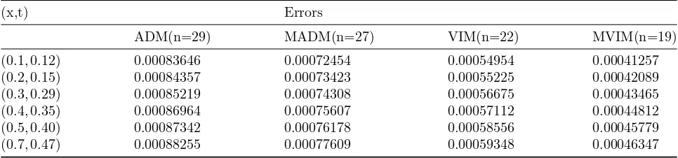
Table1, shows that, approximate solution of the Degasperis-Procesi equation is convergence with 15 iterations by using the MHPM . By comparing the results of Table 1, we can observe that the HAM is more rapid convergence than the ADM, MADM, VIM, MVIM, HPM and HAM.
5
Conclusion
Table 1: Numerical results for Example4.1
(x,t) Errors
ADM(n=29) MADM(n=27) VIM(n=22) MVIM(n=19)
(0.1,0.12) 0.00083646 0.00072454 0.00054954 0.00041257 (0.2,0.15) 0.00084357 0.00073423 0.00055225 0.00042089 (0.3,0.29) 0.00085219 0.00074308 0.00056675 0.00043465 (0.4,0.35) 0.00086964 0.00075607 0.00057112 0.00044812 (0.5,0.40) 0.00087342 0.00076178 0.00058556 0.00045779 (0.7,0.47) 0.00088255 0.00077609 0.00059348 0.00046347
(Continue Table1).
(x,t) Errors
HPM(n=20) HAM(n=17) MHPM(n=15)
(0.1,0.12) 0.00064322 0.00433885 0.00356428 (0.2,0.15) 0.00652491 0.00044475 0.00036695 (0.3,0.29) 0.00066624 0.00045513 0.00037517 (0.4,0.35) 0.00067715 0.00046729 0.00037851 (0.5,0.40) 0.00068433 0.00047146 0.00038853 (0.7,0.47) 0.00069677 0.00048572 0.00039608
this purpose, we showed that the MHPM is more rapid convergence than the ADM, MADM, VIM, MVIM, HPM and HAM.
Acknowledgments
The author would like to express her sincere ap-preciation to the Department of Mathematics, Is-lamic Azad University, Qazvin Branch for their cooperation.
References
[1] S. Abbasbandy, Numerical method for non-linear wave and diffusion equations by the variational iteration method, Q1 Int. J. Nu-mer. Methods Eng. 73 (2008) 1836-1843.
[2] S. Abbasbandy, A. Shirzadi, The varia-tional iteration method for a class of eight-order boundary value differential equations, Z. Naturforsch 63 (2008) 745-751.
[3] M. J. Ablowitz, H. Segur, Soliton and The Inverse Scattering Transformation, SIAM, Philadelphia, PA, 1981.
[4] T. A. Abassy, El-Tawil, H. El. Zoheiry, To-ward a modified variational iteration method
(MVIM) , J. Comput. Apll. Math. 207 (2007) 137-147.
[5] T. A. Abassy, El-Tawil, H. El. Zoheiry, Mod-ified variational iteration method for Boussi-nesq equation, Comput. Math. Appl. 54 (2007) 955-965.
[6] S. Abbasbandy, Modified homotopy per-turbation method for nonlinear equations and comparsion with Adomian decompo-sition method, Appl. Math. Comput 172 (2006) 431-438.
[7] S. H. Behriy, H. Hashish, I. L. E-Kalla, A. El-said,A new algorithm for the decomposition solution of nonlinear differential equations, App. Math. Comput. 54 (2007) 459-466.
[8] E. Babolian, J. Saeidian, Analytic approx-imate solutions to Burger, Fisher, Huxley equations and two combined forms of these equations, Commun Nonlinear Sci Numer Simulat. 14 (2009) 1984-1992.
[9] J. Biazar, H. Ghazvini, Convergence of the homotopy perturbation method for partial differential equations, Nonlinear Analysis: Real World Application 10 (2009) 2633-2640.
equation, J. Appl. Math. Informatics 28 (2010) 1227-1237.
[11] Sh. S. Behzadi, M. A. Fariborzi Araghi,The use of iterative methods for solving Naveir-Stokes equation, J. Appl. Math. Informatics 29 (2011) 1-15.
[12] A. Degasperis, M. Procesi, Asymptotic in-tegrability, in: Symmetry and Perturbation Theory, Rome, 1998, World Scientific, River Edge, NJ (1999) 2337.
[13] I. L. El-Kalla, Convergence of the Adomian method applied to a class of nonlinear in-tegral equations, Appl. Math. Comput. 21 (2008) 372-376.
[14] M. A. Fariborzi Araghi, Sh. S. Behzadi, Solv-ing nonlinear Volterra-Fredholm integral dif-ferential equations using the modified Ado-mian decomposition method, Comput. Meth-ods in Appl. Math. 9 ( 2009) 1-11.
[15] M. A. Fariborzi Araghi, Sh. S. Behzadi,
Solving nonlinear Volterra-Fredholm integro-differential equations using He’s variational iteration method, International Journal of Computer Mathematics http://dx.doi. org/10.1007/s12190-010-0417-4/, 2010. [16] M. A. Fariborzi Araghi, Sh. S. Behzadi,
Numerical solution of nonlinear Volterra-Fredholm integro-differential equations using Homotopy analysis method, Jour-nal of Applied Mathematics and Com-puting http://dx.doi.org/10.1080/ 00207161003770394/, 2010.
[17] M. A. Fariborzi Araghi, Sh. S. Behzadi, Nu-merical solution for solving Burger’s-Fisher equation by using Iterative Methods, Mathe-matical and Computational Applications 16 (2011) 443-455.
[18] M. Ghasemi , M. Tavasoli , E. Babo-lian,Application of He’s homotopy perturba-tion method of nonlinear integro-differential equation, Appl. Math. Comput. 188 (2007) 538-548.
[19] A. Golbabai , B. Keramati,Solution of non-linear Fredholm integral equations of the first kind using modified homotopy perturbation method, Chaos Solitons and Fractals 5 (2009) 2316-2321.
[20] F. Guo, Global weak solutions and breaking waves to the DegasperisProcesi equation with linear dispersion, J. Math. Anal. Appl. 360 (2009) 345362.
[21] M. Giuseppe Coclite , Kenneth H. Karlsen,
On the uniqueness of discontinuous solutions to the Degasperis-Procesi equation, J. Differ-ential Equations 234 (2007) 142160.
[22] J. H. He, X. H. Wu, Exp-function method for nonlinear wave equations, Chaos, Soli-tons and Fractals 30 (2006) 700-708.
[23] J. H. He,Variational principle for some non-linear partial differential equations with vari-able cofficients, Chaos, Solitons and Fractals 19 (2004) 847-851.
[24] J. H. He, Wang. Shu-Qiang,Variational iter-ation method for solving integro-differential equations, Physics Letters A 367 (2007) 188-191.
[25] J. H. He, Variational iteration method some recent results and new interpretations, J. Comp. Appl. Math. 207 (2007) 3-17.
[26] M. Javidi, Modified homotopy perturbation method for solving linear Fredholm integral equations, Chaos Solitons and Fractals 50 (2009) 159-165.
[27] B. G. Konopelchenko,Inverse spectral trans-form for the (2 + 1)-dimensional Gardner equation, Inverse Prob. 7 (1991) 739753.
[28] Z. Liu, Z. Ouyang,A note on solitary waves for modified forms of CamassaHolm and De-gasperisProcesi equations, Phys. Lett. A 366 (2007) 377381.
[29] H. Lundmark , J. Szmigielski, Degasperis-Procesi peakons and the discrete cubic string IMRP, Int. Math. Res. Pap. 2 (2005) 53116.
[30] S. J. Liao, Beyond Perturbation: Intro-duction to the Homotopy Analysis Method, Chapman and Hall/CRC Press,Boca Raton, 2003.
[32] C. Shena, A. Gaob, Optimal control of the viscous weakly dispersive Degasperis - Pro-cesi equation, Nonlinear Analysis 72 (2010) 933-945.
[33] S. A. Sezer, A.Yildirim, S. T. Mohyud-Din,
Hes homotopy perturbation method for solv-ing the fractional KdV-Burgers-Kuramoto equation, International Journal of Numerical Methods for Heat and Fluid Flow 21 (2011) 448-458.
[34] A. M. Wazwaz, Construction of solitary wave solution and rational solutions for the KdV equation by ADM, Chaos, Solution and fractals 12 (2001) 2283-2293.
[35] A. M. Wazwaz, A first course in integral equations, WSPC, New Jersey, 1997.
[36] M. Wadati, The exact solution of the modi-fied Kortweg-de Vries equation, J. Phys. Soc. Jpn. 32 (1972) 16811687.
[37] A.Yildirim, S.T. Mohyud-Din, D. H. Zhang,
Analytical solutions to the pulsed Klein-Gordon equation using Modified Variational Iteration Method (MVIM) and Boubaker Polynomials Expansion Scheme (BPES), Computers and Mathematics with Applica-tions 59 (2010) 2473-2477.
[38] A. A.Yildirim, Variational iteration method for modified Camassa-Holm and Degasperis-Procesi equations, International Journal for Numerical Methods in Biomedical Engineer-ing 26 (2010) 266-272.
[39] A. A.Yildirim,Solution of BVPs for Fourth-Order Integro-Differential Equations by us-ing Homotopy Perturbation Method, Com-puters and Mathematics with Applications 56 (2008) 3175-3180.
[40] A. A.Yildirim, The Homotopy Perturbation Method for Approximate Solution of the Modified KdV Equation, Zeitschrift fr Natur-forschung A, A Journal of Physical Sciences 63 (2008) 621-626.
[41] A. A.Yildirim, Application of the Homotopy perturbation method for the Fokker-Planck equation, International Journal for Numer-ical Methods in BiomedNumer-ical Engineering 26 (2010) 1144-1154.
[42] N. J. Zabusky, M. D. Kruskal, Interaction of Solitons in a collisionless plasma and the recurrence of initial states, Phys. Rev. Lett. 15 (1965) 240-253.