Vol. 4, No. 2, Year 2012 Article ID IJIM-00212, 12 pages Research Article
Numerical Solution of Singular IVPs of
Lane-Emden Type Using Integral Operator and
Radial Basis Functions
M. Heydaria, S.M. Hosseinib, G.B. Loghmania∗
(a)Department of Mathematics, Yazd University P.O. Box: 89195-741, Yazd, Iran.
(b)Department of Mathematics, Science and Research Branch, Islamic Azad University, Tehran, Iran. ——————————————————————————————————
Abstract
A numerical method for solving the Lane-Emden equations as singular initial value prob-lems is presented. The method is based on using integral operator and convert Lane-Emden equations to integral equations and interpolation by radial basis functions (RBFs). Also, Legendre-Gauss quadrature integration method utilized to reduce the solution of integral equations to the solution of algebraic equations. Several examples are given and numerical examples are presented to demonstrate the validity and applicability of the method.
Keywords: Lane-Emden equations; Strictly positive functions; Radial basis functions.
——————————————————————————————————
1
Introduction
Recently, a lot of attention has been focused on the study of singular initial value problems (IVPs) in the second-order ordinary differential equations (ODEs). Many problems arising in the field of mathematical physics and astrophysics can be modelled by Lane-Emden type initial value problems, which can be written in the form:
y′′+α
xy
′+f(y) = 0, 0< x≤1, α≥0, (1.1)
subject to conditions
y(0) =A, y′(0) =B, (1.2) whereAandB are constants andf(y) is a real-valued continuous function. This equation was used to model various phenomena such as the theory of stellar structure, the thermal
∗Corresponding author. Email address: [email protected]
behaviour of a spherical cloud of gas, isothermal gas spheres and the theory of thermionic currents [12, 16, 33].
On the other hand, another class of singular initial value problems of Lane-Emden type can also be given in the form:
y′′+α
xy
′+f(x, y) =g(x), 0< x≤1, α≥0, (1.3)
subject to conditions given in Eq. (1.2), where A and B are constants, f(x, y) is a continuous real valued function, and g(x) ∈ C[0,1]. Eq. (1.3) differs from the classical Lane-Emden type Eq. (1.2), for the functionf(x, y) and for the inhomogeneous termg(x). Since, Lane-Emden type equations have significant applications in many fields of the scientific and technical world, a variety of forms of f(y) have been investigated by many researchers. A discussion of the formulation of these models and the physical structure of the solutions can be found in the literature. For example, it models the thermal behavior of a spherical cloud of gas acting under the mutual attraction of its molecules and subject to the classical laws of thermodynamics [16, 38, 41] when f(y) = ym, the gravitational potential of the degenerate white-dwarf stars [12] when f(y) = (y2−C)32, the isothermal
gas spheres [16] when f(y) =ey and so on.
Recently many analytical methods have been used to solve Lane-Emden equations, the main difficulty arises in the singularity of the equation at x = 0. Currently most techniques in use for handling the Lane-Emden type problems are based on either series solutions or perturbation techniques. Bender et al. [5] handled the solution of Lane-Emden equations as well as those of a variety of nonlinear problems in quantum mechanics and astrophysics by means of perturbation methods based on the existence of a small param-eter. Approximate solutions to the above problems were presented by Shawagfeh [38] and Wazwaz [41, 42] by applying the Adomian method which provides a convergent series so-lution. Nouh [29] accelerated the convergence of a power series solution of the LaneEmden equation by using an Euler-Abel transformation and Pade approximation. Mandelzweig and Tabakin [26] applied Bellman and Kalaba’s quasilinearization method and Ramos [31] used an piecewise linearization technique based on the piecewise linearization of the Lane-Emden equation. Bozkhov and Martins [7] and later Momoniat and Harley [28] applied the Lie Group method successfully to generalized Lane-Emden equations of the first kind. Exact solutions of generalized Lane-Emden solutions of the first kind are in-vestigated by Goenner and Havas [17]. Liao [22] solved Lane-Emden type equations by applying a homotopy analysis method. He [18] obtained an approximate analytical solu-tion of the Lane-Emden equasolu-tion by applying a variasolu-tional approach which uses a semi inverse method. Ramos [32] presented a series approach to the Lane-Emden equation and gave the comparison with He’s homotopy perturbation method. The authors of this paper, Yldrm and Ozis [30] and also Chowdhury and Hashim [14] gave the solutions of a class of singular second-order IVPs of Lane-Emden type by using He’s homotopy perturbation method. Youseffi [44] converted the Lane-Emden equation to an integral equation and then using Legendre wavelets, obtained an approximate solution for 0< x≤1.
2
Radial basis functions
In this section the RBFs method is defined as a technique for interpolation of the scattered data. Some well-known radial basis functions (RBFs) are listed in Table 1. Let r be the Euclidean distance between a fixed point x∗ ∈ Rd and any x ∈ Rd i.e. ∥x−x∗∥2. A
radial function ϕ∗ = ϕ(∥x−x∗∥2) depends only on the distance between x ∈ Rd and
fixed point x∗ ∈ Rd. This property results that the radial basis function ϕ∗ is radially symmetric about x∗. It is clear that the functions in Table 1 are globally supported, infinitely differentiable and depend on a free parameter c.
Let{x0, x1, ..., xN} be a given set of distinct points in Rd. The main idea behind the use of RBFs is interpolation by translation of a single function i.e. the interpolating RBFs approximation is considered as
F(x) = N
∑
i=0
λiϕi(x), (2.4)
Table 1.
Some well-known functions that generate RBFs.
Name of function Definition
Gaussian (GA) ϕ(r) = exp (−c2r2) Hardy Multiquadric (MQ) ϕ(r) =√r2+c2
Inverse Multiquadrics (IMQ) ϕ(r) = (√r2+c2)−1
Inverse Quadric (IQ) ϕ(r) = (r2+c2)−1
where ϕi(x) =ϕ(∥x−xi∥2) and λi are unknown scalars for i= 0,1,· · · , N. Assume that we want to interpolate the given values fi =f(xi),i= 0,1,· · · , N. The unknown scalars
λi are chosen so that F(xi) =fi for i= 0,1,· · · , N which results in the following linear system of equations
AZ =f, (2.5)
where Ai,j =ϕi(xj), Z = [λ0, λ1,· · · , λN] andf = [f0, f1,· · ·, fN]. Since all applicableϕ have global support, this method produces a dense matrixA. The matrixAcan be shown to be positive definite (and therefore nonsingular) for distinct interpolation points for GA, IMQ and IQ by Schoenberg’s Theorem [37]. Also using the Micchelli Theorem [27] we can show thatA is invertible for distinct sets of the scattered points in the case of MQ.
Although the matrixAis nonsingular in the above cases, usually it is very ill-conditioned i.e. the condition number of A
produce an interpolation matrix which is well conditioned enough to be inverted in finite precision arithmetic [35].
Despite research done by many scientists to develop algorithms for selecting the values of c which produce the most accurate interpolation (e.g. see [11, 34]), the optimal choice of shape parameter is still an open question.
3
Legendre-Gauss nodes and weights
Let LM+1(x) be the Legendre polynomial of order M+ 1 on [−1,1]. Then the
Legendre-Gauss nodes are
−1< x0 < x1 <· · ·< xM <1, (3.7) where{xi}Mi=0 are the zeros ofLM+1(x). No explicit formulas are known for the pointsxi, and so they are computed numerically using subroutines [10]. Also we approximate the integral off on [−1,1] as
∫ 1
−1
f(x)dx≃
M
∑
i=0
wif(xi), (3.8)
where xi are Legendre-Guass nodes in Eq. (3.7) and the weights wi given in [10]
wi =
2 (1−x2
i)[L′M+1(xi)]2
, i= 0,1,· · ·, M. (3.9)
It is well known [21] that the integration in Eq. (3.8) is exact wheneverf(x) is a polynomial of degree ≤2M + 1.
4
Solution of the problem via radial basis functions
Consider the Lane-Emden equations given in Eq. (1.3). Define integral operator
L(.) =
∫ x
0
t−α
∫ t
0
sα(.)dsdt. (4.10)
Operating withL on Eq. (1.3), it then follows:
y(x) =A+L(g(x))−L(f(x, y)), (4.11) where
A=y(0). (4.12)
Let
G(x) =A+L(g(x)), (4.13) and
F(t, y(t)) =−t−α
∫ t
0
So, we can get
y(x) =G(x) +
∫ x
0
F(t, y(t))dt, (4.15)
which is nonlinear Volterra integral equation. Let ϕ(x) be a radial basis function and we approximate y(x) with interpolation by functionϕ(x) i.e.,
y(x)≃ N
∑
j=0
cjϕ(x−xj) =CTΨ(x), (4.16)
where C and Ψ(x) are (N+ 1)×1 matrices given by
C = [c0, c1,· · ·cN]T, Ψ(x) = [ϕ(x−x0), ϕ(x−x1),· · ·ϕ(x−xN)]T. Also xj are shifted the Chebyshev-Gauss-Radau nodes on [0,1]
xj = 1 2cos
(
2πj
2N + 1
)
+1
2, j= 0,1,· · ·, N. (4.17) Now by substituting Eq. (4.16) in Eq. (4.15) we have:
CTΨ(x) =G(x) +
∫ x
0
F(t, CTΨ(t))dt. (4.18) For obtainingcj,j= 0,1,· · · , N in the above equation, by collocating at the pointsx=xi fori= 0,1,· · ·, N we have:
CTΨ(xi) =G(xi) +
∫ xi
0
F(t, CTΨ(t))dt. (4.19)
By change of variable t= xi
2(τ+ 1), Eq. (4.19) can be written as:
CTΨ(xi) =G(xi) +xi 2
∫ 1
−1
F(xi
2(τ+ 1), C TΨ(xi
2(τ+ 1)))dτ. (4.20) By applying numerical integration method given in Eq. (3.8), we can approximate the integral in Eq. (4.20) and hence the above equation can be written as follow:
CTΨ(xi) =G(xi) +
xi 2
M
∑
k=0
wkF(
xi
2(τk+ 1), C TΨ(xi
2(τk+ 1))), (4.21) for i= 0,1,· · ·, N and wk are given in Eq. (3.9). From (4.14) and numerical integration method given in Eq. (3.8), we obtain:
F(xi
2(τk+ 1), C TΨ(xi
2(τk+ 1)))≃ − [xi
2(τk+ 1)] 1−α
2
M
∑
p=0
wp[ξ(k,pi)] αf(ξ(i)
k,p, C
TΨ(ξ(i)
k,p))(4.22),
where ξ(k,pi) = xi
4(τk+ 1)(τp+ 1). So by substituting Eq. (4.22) in Eq. (4.21) we have:
CTΨ(xi) =G(xi) +
xi 2 M ∑ k=0 M ∑ p=0
where
wk,p(i) =−[ xi
2(τk+ 1)] 1−α
2 [ξ
(i)
k,p] αw
p. (4.24)
This is a nonlinear system of equations that can be solved via Newton’s iteration method to obtain unknown vectorCT.
5
Numerical examples
We use the method presented in this paper to solve four examples given in [30, 14, 43, 20, 1, 15, 4]. By choosing appropriate Radial basis function ϕ(x) and shape parameter c
we can get high accurate solution and best choice of the ϕ(x) depends on the form of the problem. In all examples, we use GA-RBF and MQ-RBF and also we use the maximum errors for differentN which is given as
E∞=max{|y(x)− N
∑
j=0
cjϕ(x−xj)|:x∈[0,1]}.
All of the computations have been done using the Maple 13 with 150 digits precision,
M = 10 and we solved obtained system by Newton’s iteration method with start point [0,0, ...,0].
Error Analysis: Madych have proven exponential convergence property of multiquadratic approximation [23]. He has shown that under certain conditions, the interpolation error is
ε=O(λhc) wherecis the shape parameter,his the mesh size and 0< λ <1 is a constant.
It implies we can improve the approximated solution either by reducing the size of h or by increasing the magnitude of c. It means that ifc→ ∞thenε→0. Since increasing of
ccan improve the accuracy exponentially without extra computation [13, 19, 23, 24], it is preferred to decrease error rather than reducing h.
However, according to ’uncertainty principle’ of Schaback [36], as the error becomes smaller, the matrix becomes more ill-conditioned; hence the solution will break down as
c becomes too large. The experimental results confirm such behavior of the error values as c becomes larger. The numerical results for Examples 1,2 and 3 on interval [0,1] are demonstrated in Fig.s 2 and 3, which show according to the findings of Madych, the error functions decrease exponentially as cbecomes larger in bounded interval. After that according to the research of Schaback the error values decline as cbecomes too large. The bestc is different for various problems and not the same RBFs.
Example 5.1. Consider the homogeneous Lane-Emden type equation [14, 43, 20, 1]
y′′+2
xy
′−(4x2+ 6)y = 0, 0< x≤1, (5.25)
subject to conditions
y(0) = 1, y′(0) = 0. (5.26)
This type of equation has been solved by [14, 43, 20, 1] with the homotopy-perturbation method, variational iteration method, power series with Pad´e approximation and modified Legendre-spectral method respectively.
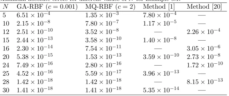
In Table 2, we list the results obtained by the RBF collocation method proposed in this paper with GA-RBF (c= 0.001) and MQ-RBF (c= 2). Also we contrast our results with the corresponding results reported by Karimi Vanani et al. [20] and Adibi et al. [1].
Table 2.
Maximum absolute errors for different values ofN for Example 5.1.
N GA-RBF (c= 0.001) MQ-RBF (c= 2) Method [1] Method [20] 5 6.51×10⁻⁴ 1.35×10⁻³ 7.80×10⁻⁴ —
10 2.15×10⁻⁸ 7.80×10⁻⁷ 1.17×10⁻⁵ —
12 2.51×10⁻¹⁰ 3.52×10⁻⁸ — 2.26×10⁻⁴ 15 2.44×10⁻¹³ 3.58×10⁻¹⁰ 1.40×10⁻⁸ —
16 2.30×10⁻¹⁴ 7.54×10⁻¹¹ — 3.05×10⁻⁶
20 5.38×10⁻¹⁵ 1.53×10⁻¹³ 3.59×10⁻¹⁰ 2.73×10⁻⁸ 24 7.49×10⁻¹⁶ 2.80×10⁻¹⁶ — 1.72×10⁻¹⁰ 25 4.52×10⁻¹⁶ 5.59×10⁻¹⁷ 3.96×10⁻¹³ —
28 1.42×10⁻¹⁸ 1.42×10⁻¹⁸ — 8.15×10⁻¹³ 30 1.41×10⁻¹⁸ 1.41×10⁻¹⁸ 5.35×10⁻¹⁴ —
From the contents of Table 3, it is clear that the choice of the shape parameter has an auxiliary role in the stability of the problem.The dimension of matrix A should be small sufficiently to guarantee the stability of the solution of the resulted linear system.
Table 3.
Some values of shape parameterc,k∞(A) using GA-RBF withN = 18 for Example 5.1. Shape parameter c E∞ k∞(A) 0.05 0.1672×10⁻¹⁵ 0.5149×1079 0.1 0.1872×10⁻¹⁵ 0.7492×1068
1 0.4748×10⁻¹³ 0.8409×1032 5 0.9163×10⁻⁴ 0.1671×10¹⁰ 10 0.1947×10⁻¹ 0.7006×10⁶
30 0.8709 0.2528×10³
Example 5.2. Consider the nonhomogeneous Lane-Emden equation [30, 15, 4, 6]
y′′+ 8
xy
′+xy =x5−x4+ 44x2−30x, 0< x≤10, (5.27)
subject to conditions
y(0) = 0, y′(0) = 0, (5.28)
for which the exact solution is y(x) =x4−x3.
Table 4.
Some values of shape parameterc,k∞(A) using GA-RBF withN = 18 for Example 5.2.
x GA-RBF (c= 0.001) MQ-RBF (c= 1000) SJC(α=β = −21) SJC(α= 12, β= −21) 0 3.46×10⁻²⁰ 7.85×10⁻¹⁸ 4.54×10⁻¹³ 1.13×10⁻¹³
1 2.78×10⁻²⁰ 7.52×10⁻¹⁸ 4.54×10⁻¹³ 1.13×10⁻¹³ 2 2.53×10⁻²⁰ 7.82×10⁻¹⁸ 0 5.68×10⁻¹⁴ 3 2.60×10⁻²⁰ 8.84×10⁻¹⁸ 6.82×10⁻¹³ 2.86×10⁻¹⁴ 4 1.84×10⁻²⁰ 6.68×10⁻¹⁸ 0 5.68×10⁻¹⁴ 5 7.47×10⁻²² 1.18×10⁻¹⁹ 1.13×10⁻¹³ 0
6 2.12×10⁻²⁰ 8.95×10⁻¹⁸ 4.54×10⁻¹³ 2.27×10⁻¹³ 7 3.82×10⁻²⁰ 1.64×10⁻¹⁷ 0 0
8 4.46×10⁻²⁰ 1.96×10⁻¹⁷ 0 0 9 5.20×10⁻²⁰ 2.33×10⁻¹⁷ 0 0 10 6.65×10⁻²⁰ 3.04×10⁻¹⁷ 0 0
Example 5.3. (The isothermal gas spheres equation) Consider the nonlinear, homoge-neous Lane-Emden type equation [15, 4, 2, 3]
y′′+ 2
xy
′+ey = 0, 0< x≤2.5, (5.29)
subject to conditions
y(0) = 0, y′(0) = 0. (5.30) A series solution obtained by Wazwaz [41], Liao [22], Singh et al. [39] and Ramos [32] by using ADM, HAM, MHAM and series expansion respectively:
y(x)≃ −1 6x
2+ 1
5.4!x
4− 8
21.6!x
6+ 122
81.8!x
8− 61.67
495.10!x
10. (5.31)
Table 5 shows the comparison ofy(x) obtained by the RBF method proposed in this paper with (GA-RBF ,N = 10, c= 0.3) and those obtained by Wazwaz [41].
The resulting graph of the isothermal gas spheres equation in comparison to the pre-sented method and those obtained by Wazwaz [41] is shown in Fig. 1.
Table 5.
Comparison between present method and Wazwaz method [41].
x GA-RBF (c= 0.3) Wazwaz [41] Error 0.0 0.0000000000 0.0000000000 0.0
0.1 -0.0016658328 -0.0016658338 9.91×10⁻¹⁰
0.2 -0.0066533691 -0.0066533671 2.07×10⁻⁹ 0.5 -0.0411539552 -0.0411539568 1.55×10⁻⁹ 1.0 -0.1588276770 -0.1588273536 2.23×10⁻⁷
Fig. 1. Graph of isothermal gas sphere equation in comparison with Wazwaz solution [41].
Fig. 2. Horizontal axis is related to shape parameter (c) and vertical axis shows error values with
log mode when the solutions are approximated by using GA-RBF withN = 10 on interval [0,1].
Fig. 3. Horizontal axis is related to shape parameter (c) and vertical axis shows error values with
6
Conclusion
The aim of present work is to develop an efficient and accurate method for solving the Lane-Emden equations as singular initial value problems. The properties of the radial basis functions together with the Gaussian integration method are used to reduce the problem to the solution of nonlinear algebraic equations. This technique is very simple, the elements of system can be obtained easily and involve less computation. The illustrative example confirm the validity of the method.
References
[1] H. Adibi , AM. Rismani, On using a modified Legendre-spectral method for solving singular IVPs of Lane-Emden type, Comput. Math. Appli. 60 (2010) 2126-2130. [2] A. Aslanov, Determination of convergence intervals of the series solutions of
Emden-Fowler equations using polytropes and isothermal spheres, Phys. Lett. A 372 (2008) 3555-3561.
[3] A. Aslanov, A generalization of the LaneEmden equation, Int. J. Comput. Math. 85 (2008) 1709-1725.
[4] AS. Bataineh, MSM. Noorani, I. Hashim, Homotopy analysis method for singular IVPs of Emden-Fowler type, Commun. Nonlinear. Sci. Numer. Simul. 14 (2009) 1121-1131.
[5] CM. Bender, KA. Milton, SS. Pinsky, LM. Simmons, A new perturbation approach to nonlinear problems, J. Math. Phys. 30 (1989) 1447-1455.
[6] AH. Bhrawy, AS. Alofi, A JacobiGauss collocation method for solving nonlinear La-neEmden type equations, Commun. Nonlinear. Sci. Numer. Simul. 17 (2012) 62-70. [7] Y. Bozkhov, ACG. Martins, Lie point symmetries and exact solutions of quasilinear
differential equations with critical exponents, Nonlinear Anal. 57 (2004) 773-793. [8] MD. Buhmann, Spectral convergence of multiquadric interpolation, Proc. Edinburg.
Math. Soc. 36 (1993) 319-333.
[9] MD. Buhmann, Radial Basis Functions, Cambridge University Press, Cambridge, 2003.
[10] C. Canuto, MY. Hussaini, A. Quarteroni, TA. Zang, Spectral Methods in Fluid Dy-namics, Springer-Verlag, New York, 1988.
[11] RE. Carlson, TA. Foley, Interpolation of track data with radial basis functions, Com-put. Math. Appl. 24 (1992) 27-34.
[12] S. Chandrasekhar, Introduction to the Study of Stellar Structure, Dover, New York, 1967.
[14] MSH. Chowdhury, I. Hashim, Solutions of a class of singular second-order IVPs by homotopy-perturbation method, Phys. Lett. A. 368 (2007) 305-313.
[15] MSH. Chowdhury, I. Hashim, Solutions of Emden-Fowler equations by homotopy perturbation method, Nonlinear Anal. 10 (2009) 104-115.
[16] HT. Davis, Introduction to Nonlinear Differential and Integral Equations, Dover, New York, 1962.
[17] H. Goenner, P. Havas, Exact solutions of the generalized Lane-Emden equation, J. Math. Phys. 41 (2000) 7029-7042.
[18] JH. He, Variational approach to the Lane-Emden equation, Appl. Math. Comput. 143 (2003) 539-541.
[19] C-S. Huang, CF. Lee, AH-D. Cheng, Error estimate, optimal shape factor, and high precision computation of multiquadric collocation method, Eng. Anal. Boundary Elem. 31 (2007) 614-623.
[20] S. Karimi Vanani, A. Aminataei, On the numerical solution of differential equations of Lane-Emden type, Comput. Math. Appli. 59 (2010) 2815-2820.
[21] C. Kui-Fang, Strictly positive definite functions, J. Approx. Theory. 87 (1996) 148-158.
[22] S. Liao, A new analytic algorithm of Lane-Emden type equations, Appl. Math. Com-put. 142 (2003) 1-16.
[23] WR. Madych, Miscellaeous error bounds for multiquadratic and related interpolators, Comput. Math. Appl. 24 (1992) 121-138.
[24] WR. Madych, Bounds on multivariate polynomials and exponential error estimates for multiquadric interpolation, J. Approx. Theory. 70 (1992) 94-114.
[25] WR. Madych, S.A. Nelson, Multivariate interpolation and conditionally positive def-inite functions, II, Math. Comput. 54 (1990) 211-230.
[26] VB. Mandelzweig, F. Tabakin, Quasilinearization approach to nonlinear problems in physics with application to nonlinear ODEs, Comput. Phys. Commun. 141 (2001) 268-281.
[27] CA. Micchelli, Interpolation of scattered data: Distance matrices and conditionally positive definite functions, Constructive Approximation 2 (1986) 11-22.
[28] E. Momoniat, C. Harley, Approximate implicit solution of a Lane-Emden equation, New Astron. 11 (2006) 520-526.
[29] MI. Nouh, Accelerated power series solution of polytropic and isothermal gas spheres, New Astron. 9 (2004) 467-473.
[31] JI. Ramos, Linearization method in classical and quantum mechanics, Comput Phys. Commun. 153 (2003) 199-208.
[32] JI. Ramos, Series approach to the LaneEmden equation and comparison with the homotopy perturbation method, Chaos Solitons Fractals 38 (2008) 400-408.
[33] OU. Richardson, The Emission of Electricity from Hot Bodies, Zongmans Green and Company, London, 1921.
[34] S. Rippa, An algorithm for selecting a good parameter c in radial basis function interpolation, Adv. Comput. Math. 11 (1999) 193-210.
[35] SA. Sarra, Adaptive radial basis function method for time dependent partial differ-ential equations, Appl. Numer. Math. 54 (2005) 79-94.
[36] R. Schaback, Error estimate and condition numbers for radial basis function interpo-lation, Adv. Comput. Math. 3 (1995) 251-264.
[37] IJ. Schoenberg, Metric spaces and completely monotone functions, Annals of Math-ematics 39 (1938) 811-841.
[38] NT. Shawagfeh, Nonperturbative approximate solution for Lane-Emden equation, J. Math. Phys. 34 (9) (1993) 4364-4369.
[39] OP. Singh, R.K. Pandey, V.K. Singh, An analytic algorithm of LaneEmden type equations arising in astrophysics using modified homotopy analysis method, Comput. Phys. Commun. 180 (2009) 1116-1124.
[40] AR. Vahidi, M. Didgar, Improving the Accuracy of the Solutions of Riccati Equations, Int. J. Industrial. Mathematics. 4 (2012) 11-20.
[41] AM. Wazwaz, A new algorithm for solving differential equations of Lane-Emden type, Appl. Math. Comput. 118 (2001) 287-310.
[42] AM. Wazwaz, A new method for solving singular value problems in the second order ordinary differential equations, Appl. Math. Comput. 128 (2001) 45-57.
[43] A. Yldrm, T. Ozis, Solutions of singular IVPs of Lane-Emden type by the variational iteration method, Nonlinear Anal. 70 (2009) 2480-2484.

![Fig. 3. Horizontal axis is related to shape parameter (c) and vertical axis shows error values withlog mode when the solutions are approximated by using MQ-RBF with N = 10 on interval [0, 1].](https://thumb-us.123doks.com/thumbv2/123dok_us/8878420.1818254/9.595.209.392.113.296/horizontal-related-parameter-vertical-withlog-solutions-approximated-interval.webp)
