From wind to loads: wind turbine site-specific load estimation with surrogate models trained on high-fidelity load databases

(1)

https://doi.org/10.5194/wes-3-767-2018

From wind to loads: wind turbine site-specific

load estimation with surrogate models

trained on high-fidelity load databases

Nikolay Dimitrov, Mark C. Kelly, Andrea Vignaroli, and Jacob Berg

DTU Wind Energy, Technical University of Denmark, Risø Campus, Frederiksborgvej 399, 4000 Roskilde, Denmark

Correspondence:Nikolay Dimitrov ([email protected])

Received: 16 February 2018 – Discussion started: 2 March 2018

Revised: 22 August 2018 – Accepted: 26 September 2018 – Published: 24 October 2018

Abstract. We define and demonstrate a procedure for quick assessment of site-specific lifetime fatigue loads using simplified load mapping functions (surrogate models), trained by means of a database with high-fidelity load simulations. The performance of five surrogate models is assessed by comparing site-specific lifetime fa-tigue load predictions at 10 sites using an aeroelastic model of the DTU 10 MW reference wind turbine. The surrogate methods are polynomial chaos expansion, quadratic response surface, universal Kriging, importance sampling, and nearest-neighbor interpolation. Practical bounds for the database and calibration are defined via nine environmental variables, and their relative effects on the fatigue loads are evaluated by means of Sobol sen-sitivity indices. Of the surrogate-model methods, polynomial chaos expansion provides an accurate and robust performance in prediction of the different site-specific loads. Although the Kriging approach showed slightly better accuracy, it also demanded more computational resources.

1 Introduction

Before installing a wind turbine at a particular site, it needs to be ensured that the wind turbine structure is sufficiently ro-bust to withstand the environmentally induced loads during its entire lifetime. As the design of serially produced wind turbines is typically based on a specific set of wind condi-tions, i.e., a site class defined in the IEC (2005) standard, any site where the conditions are more benign than the ref-erence conditions is considered feasible. However, often one or more site-specific parameters will be outside this envelope – and disqualify the site as infeasible unless it is shown that the design load limits are not going to be violated under site-specific conditions. Such a demonstration requires carrying out simulations over a full design load basis, which adds a significant burden to the site assessment process.

Various methods and procedures have been attempted for simplified load assessment for wind energy applications. Kashef and Winterstein (1999) and Manuel et al. (2001) use probabilistic expansions based on statistical moments.

(2)

and Graf et al. (2016). An alternative to the surrogate model-ing approach discussed in this paper could be the load set re-duction, as described in, for example, Häfele et al. (2018) and Zwick and Muskulus (2016), which also reduces the num-ber of simulations required. This approach, however, still re-quires carrying out high-fidelity simulations that leads to us-ing more time for simulation setup, computations, and post-processing, while with a surrogate model the lifetime equiva-lent load computation takes typically less than a minute on a regular personal computer. The studies most in line with the scope of the present paper are those by Müller et al. (2017), Teixeira et al. (2017), and Toft et al. (2016). The former two employ advanced surrogate modeling techniques (arti-ficial neural networks and Kriging, respectively); however, the experimental designs are relatively small and with a lim-ited range of variation for some of the variables, and the dis-cussion does not focus on the practical problem of comput-ing lifetime-equivalent site-specific loads. The computation of site-specific lifetime-equivalent design loads is the main focus in Toft et al. (2016), but with a limited number of vari-ables and using a low-order quadratic response surface. The vast majority of the studies employ a single surrogate mod-eling approach, meaning that it has not been possible to di-rectly compare the performance of different approaches.

In the present work, we analyze, refine, and expand the existing simplified load assessment methods, and provide a structured approach for practical implementation of a surro-gate modeling approach for site feasibility assessment. The study aims at fulfilling the following four specific goals:

– define a simplified load assessment procedure that can take into account all the relevant external parameters re-quired for full characterization of the wind fields used in load simulations;

– define feasible ranges of variation in the wind-related parameters, dependent on wind turbine rotor size;

– demonstrate how different surrogate modeling ap-proaches can be successfully employed in the problem, and compare their performance; and

– obtain estimates of the statistical uncertainty and param-eter sensitivities.

The scope of the present study is loads generated un-der normal power production, which encompasses design load cases (DLCs) 1.2 and 1.3 from the IEC 61400-1 stan-dard (IEC, 2005). These load cases are the main contribu-tors to the fatigue limit state (DLC1.2) and often the blade extreme design loads (DLC1.3) (Dimitrov et al., 2017; Bak et al., 2013). The methodology used can easily be applied to other load cases governed by wind conditions with a probabilistic description. Loads generated during fault ditions (e.g., grid drops) or under deterministic wind con-ditions (e.g., operational gusts without turbulence) will in

general not be (wind climate) site-specific. The loads anal-ysis is based on the DTU 10 MW reference wind tur-bine (Bak et al., 2013) simulated using the Hawc2 software (Larsen and Hansen, 2012).

2 Definition of the surrogate load modeling

procedure

2.1 Schematic description

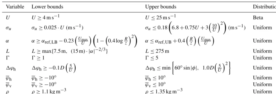
Figure 1 shows a schematic overview of the procedure for site-specific load assessment using simplified load mapping functions (here referred to in general as surrogate models). The main advantage of this procedure is that the computa-tionally expensive high-fidelity simulations are only carried out once, during the model training process (top of Fig. 1). In the model deployment process (bottom of Fig. 1), only the coefficients of the trained surrogate models are used, and a site-specific load evaluation typically takes less than a minute on a standard personal computer.

2.2 Definition of variable space

The turbulent wind field serving as input to aeroelastic load simulations can be fully statistically characterized by the fol-lowing variables:

– mean wind field across the rotor plane as described by the

– average wind speed at hub height,U;

– vertical wind shear exponent,α;

– wind veer (change of mean flow direction with height,1ϕ);

– turbulence described via

– variance of wind fluctuations,σ_u2;

– turbulence probability density function (e.g., Gaus-sian);

– turbulence spectrum defined by the Mann (1994) model with parameters

– turbulence length scaleL, – anisotropy factor0,

– turbulence dissipation parameterαε2/3;

– air densityρ;

– mean wind inflow direction relative to the turbine in terms of

– vertical inflow (tilt) angleϕ_vand

(3)

Pseudo-random sequence generation Definition of

variable set

Training set: uniform, uncorrelated sample of environmental

conditions

HAWC2 simulations

High-fidelity load database: statistics

and damage-equivalent loads

Input definition Load data generation

Model training Least-squares,

LASSO

Surrogate model coefficients

Surrogate model training

Fatigue analysis Rainflow counting

Variable sensitivities

Pseudo-random sequence generation Site-specific joint

distribution of environmental conditions

Evaluation set: site-specific conditions MC sample

Numerical integration

Lifetime equivalent site-specific design

loads

Site-specific MC sample Integration

Training process

Model deployment

Surrogate model

evaluation Site-specific load MC sample

Site-specific MC sample (surrogate)

Figure 1.Schematic overview of the site-specific load analysis procedure.

All the quantities referred to above are considered in terms of 10 min average values. All variables, except the variables defining mean inflow direction, are probabilistic and site-dependent in nature. The mean inflow direction variables rep-resent a combination of deterministic factors (i.e., terrain in-clination or yaw direction bias in the turbine) and random fluctuations due to, for example, large-scale turbulence struc-tures or variations in atmospheric stability. Mean wind speed, turbulence, and wind shear are well known to affect loads and are considered in the IEC 61400-1 standard. In Kelly et al. (2014) a conditional relation describing the joint probability of wind speed, turbulence, and wind shear was defined. The effect of implementing this wind shear distribution in load simulations was assessed in Dimitrov et al. (2015), showing that wind shear has importance especially for blade deflec-tion. The Mann model parametersLand0were also shown to have a noticeable influence on wind turbine loads (Dim-itrov et al., 2017). By definition, for a given combination ofL

and0, theαε2/3parameter from the Mann model is directly proportional toσ_u2L−2/3(Mann, 1994; Kelly, 2018), and can therefore be omitted from the analysis. The probability den-sity function (pdf) typically used to synthesize time series of velocity components from the Mann model spectra is Gaus-sian. For a slightly smaller turbine, the NREL (National Re-newable Energy Laboratory) 5 MW turbine, the assumption of Gaussian turbulence has been shown to not impact the fa-tigue loads (Berg et al., 2016). The final list of inflow-related parameters thus reads as (see Table 1 for details)

{U, σu, α, L, 1ϕ, 0, ϕh, ϕv, ρ}.

The loads experienced by a wind turbine are a func-tion of the wind-derived factors described above, and of the structural properties and control system of the wind turbine. Therefore, a load characterization database taking only wind-related factors into account is going to be turbine-specific.

The variables describing the wind field often have a sig-nificant correlation between them, and any site-specific load or power assessment has to take this into account using an

appropriate description of the joint distribution of input vari-ables. At the same time, most probabilistic models require inputs in terms of a set of independent and identically dis-tributed (i.i.d) variables. The mapping from the space of i.i.d variables to joint distribution of physical variables requires applying an isoprobabilistic transformation as, for example, the Nataf transform (Liu and Der Kiureghian, 1986) or the Rosenblatt transformation (Rosenblatt, 1952). In the present case, it is most convenient to apply the Rosenblatt transfor-mation, because it allows for more complex conditional de-pendencies than the Nataf transformation that implies linear correlation. The Rosenblatt transformation maps a vector of

ndependent variablesXinto a vector of independent com-ponentsYbased on conditional relations:

X→Y= 

      

F1(X1)

.. .

Fk|1,...,k−1(Xk|X1, . . ., Xk−1)

.. .

Fn|1,...,n−1(Xn|X1, . . ., Xn−1)



      

. (1)

Further mapping ofYto a standard normal space vectorUis sometimes applied, i.e.,

Y→U= 



8−1(Y1)

. . . 8−1(Yn)



. (2)

(4)

Table 1.Bounds of variation for the variables considered. All values are defined as statistics over 10 min reference period.

Variable Lower bounds Upper bounds Distribution

U U≥4 m s−1 U≤25 m s−1 Beta

σu σu≥0.025·U(m s−1) σu≤0.18

6.8+0.75U+310_U2

(m s−1) Uniform

α α≥αref,LB−0.23

Umax

U

1−0.4 logR_z2

α≤αref,UB+0.4

R

z Umax

U

Uniform

L L≥max{7.5 m, (15 m)· |α|−2/3} L≤275 m Uniform

0 0≥1 0≤5 Uniform

1ϕh 1ϕh≥ −0.1D

5

U

1ϕh≤min

60◦sin|φ|, 1.0D

5

U 2

Uniform

ϕh ϕh≥ −10◦ ϕh≤10◦ Uniform

ϕ_v ϕ_v≥ −10◦ ϕ_v≤10◦ Uniform

ρ ρ≥1.1 kg m−3 ρ≤1.35 kg m−3 Uniform

Where

–Ris the rotor radius,Dthe rotor diameter;

–αref,LB=0.15, αref,UB=0.22 are reference wind shear exponents at 15 m s−1wind speed;

–Umax=25 m s−1is the upper bound of the wind speed;

–φis the reference latitude (here chosen as 50◦).

2.3 Defining the ranges of input variables

The choice for ranges of variation in the input variables needs to ensure a balance between two objectives: (a) covering as wide a range of potential sites as possible, while (b) ensur-ing that the load simulations produce valid results. To ensure validity of load simulations, the major assumptions behind the generation of the wind field and computation of aerody-namic forces should not be violated, and the instantaneous wind field should have physically meaningful values.

For the case of building a high-fidelity load database, all variables given in Table 1 except the wind speed are uni-form, and only the distribution bounds are conditionally de-pendent on other variables as specified by the second and third columns of the table. The bounds of several variables are conditional on the wind speed, and as shown on Fig. 2 they are wider at low wind speeds, meaning that more sam-ple points are needed to cover the space evenly. This dictates that the choice of distribution for the wind speed should pro-vide more samples at low wind speeds. In the present study we have selected a beta distribution, but other choices such as a truncated Weibull are also feasible.

The turbulence intensity, Iu=σu/U,upper limit can be

written as the IEC-prescribed form (ed. 3, subclass A) with

Iref,A=18 %, plus a constant (representing the larger

ex-pected range of TI, to span different sites) and a term that encompasses low wind speed sites and regimes which have higher turbulent intensities. This form is basically equivalent to σu,IEC+Iref,AUcut-in[1+(Ucut-out/U)] with

{Ucut-in, Ucut-out}={4,25} m s−1. The bounds for turbulence

intensity as a function of mean wind speed are shown in Fig. 2. The limits on shear exponent were chosen follow-ing the derivations and findfollow-ings of Kelly et al. (2014) for

P(α|U), expanding on the established σα(U) form to

al-low for a reasonably wide and inclusive range of expected cases, and also accounting for rotor size per height above ground. This includes an upper bound that allows for en-hanced shear due to, for example, lower-level jets and terrain-induced shear; the lower bound also includes theR/z de-pendence, but does not expand the space to the point that it includes jet-induced negative shear (these are generally found only in the top portion of the rotor). The condition

L >max{7.5 m,(15 m)|α|−2/3}arises from consideration of the relationship betweenL, α, σu, andε; small shear tends

to correlate with larger motions (as in convective well-mixed conditions), asL'zIu/α(Kelly, 2018). The minimum scale

(7.5 m) and proportionality constant (15 m) are set to allow a wide range of conditions (though most sites will likely have a scaling factor larger than 15 m). The maximum Mann model length scale is chosen based on the limits of where the model can be fitted to measured spectra; this is also dictated by the limits of stationarity in the atmospheric boundary layer (and applicability of Taylor’s hypothesis). The range of0is also dictated by the minimum expected over non-complex terrain within reasonable use of the turbulence model (smaller 0

might occur for spectra fitted at low heights over hills, but such spectra should be modeled in a different way, as in for example Mann, 2000). The range of veer is limited in a way analogous to shear exponent, i.e., it has a basic 1/U depen-dence; this range also depends upon the rotor size, just as

(dU/dz)|_rotor=αD/U (Kelly and van der Laan, 2018). The

limits for1ϕhabove peak follow from the limits onα, while

for unstable conditions (1ϕh< 1ϕh,peak, e.g., all 1ϕh<0)

then the veer limit follows a semi-empirical form based on observed extremes of∂ϕh/∂z. For the remaining variables,

(5)

they are wide enough to encompass the values typically used in a design load basis.

2.4 Sampling procedure

Building a large database with high-fidelity load simulations covering the entire variable space is a central task in the present study as such a database can serve several purposes:

1. be directly used as a site assessment tool by probability weighting the relative contribution of each point to the design loads;

2. serve as an input for calibrating simplified models, i.e., surrogate models and response surfaces.

Characterizing the load behavior of a wind turbine over a range of input conditions requires an experimental design covering the range of variation in all variables with sufficient resolution. In the case of having more than 3–4 dimensions, a full factorial design with multiple levels quickly becomes impractical due to the exponential increase in the number of design points as a function of the number of dimensions. Therefore, in the present study we resort to a MC simula-tion as the main approach for covering the joint distribu-tion of wind condidistribu-tions. For assuring better and faster con-vergence, we use the low-discrepancy Halton sequence in a quasi-MC approach (Caflisch, 1998). While a crude MC inte-gration has a convergence rate proportional to the square root of the number of samplesN, i.e., the mean errorε∝N−0.5, the convergence rate for a quasi-MC with a low-discrepancy sequence results in ε∝N−λ, 0.5≤λ≤1. For a low num-ber of dimensions and smooth functions, the quasi-MC se-quences show a significantly improved performance over the MC sequences, e.g., λ→1; however, for multiple dimen-sions and discontinuous functions, the advantage over crude MC is reduced (Morokoff and Caflisch, 1995). Neverthe-less, even for the full 9-dimensional problem discussed here, it is expected that λ≈0.6 (Morokoff and Caflisch, 1995), which still means about an order of magnitude advantage, e.g., 104quasi-MC samples should result in about the same error as 105crude MC samples. A disadvantage of the quasi-random sequences is that their properties typically deteri-orate in high-dimensional problems, where periodicity and correlation between points in different dimensions may ap-pear (Morokoff and Caflisch, 1995). However, such behav-ior typically occurs when more than 20–25 dimensions are used. In the present problem the dimensionality is limited by the computational requirements of the surrogate models and the aeroelastic simulations used to train them. Therefore the behavior of quasi-random sequences in high dimensions does not have implications for the present study. The Halton sequence is applied by consequentially taking all points in the quasi-random series without omission and without rep-etitions, starting from the second point. The first point in the sequence is discarded as it contains zeros (i.e., the lower

bounds of the interval[0,1]) in all dimensions, which corre-sponds to zero joint probability for the input variablesX.

2.5 Database specification

A large-scale generic load database is generated in order to serve as a training data set for the load mapping functions. The point sampling is done using a Halton low-discrepancy sequence within the 9-dimensional variable space defined in Sect. 2.4 (Fig. 2 shows the bounds for the first six variables). The database setup is the following:

– Up to 104 quasi-random MC sample points in the in-terval[0,1) are generated, following a low-discrepancy sequence for obtaining evenly distributed points within the parametric space.

– The physical values of the stochastic variables for all quasi-MC samples are obtained by applying a Rosen-blatt transformation using the conditional distribution bounds given in Table 1 and using uniform distribution density, except for the wind speed for which a beta dis-tribution is used.

– For each sample point, eight simulations, with 3800 s duration each, are carried out. The first 200 s of the sim-ulations are discarded in order to eliminate simulation run-in time transients, and the output is 3600 s (1 h) of load time series from each simulation.

– The Mann model simulation parameters (L,0,α2/3) that determine the turbulence intensity are tuned to match the required 10 min turbulence statistics (1 h statistics are slightly different due to longer sampling time).

– Each 1 h time series is split into six 10 min series, which on average will have the required statistics. This leads to a total of 48 10 min time series for each quasi-MC sample point.

– Simulation conditions are kept stationary over each 1 h simulation period.

– The DTU 10 MW reference wind turbine model (Bak et al., 2013), with the basic DTU Wind Energy con-troller (Hansen and Henriksen, 2013), is used in the Hawc2 aeroelastic software (Larsen and Hansen, 2012).

(6)

Figure 2.Sample distributions obtained using 1024 low-discrepancy points within a 6-dimensional variable space{U, Iu, α, 1φh, L, 0}.

Here U is beta-distributed, while the other variables are uniformly distributed within their ranges. Solid lines show the sampling space bounds, which are curved due to conditional dependencies. Blue shading shows the site-specific variable distribution for the Nørrekær Enge (NKE) reference site (site 0, cf. Table 5 and Sect. 6.1).

3 Post-processing and analysis

3.1 Time series postprocessing and cycle counting The main quantities of interest from the load simulation out-put are the short-term (10 min) fatigue damage-equivalent loads (DELs), and the 10 min extremes (minimum or max-imum, depending on the load type). For each load simula-tion, four statistics (mean, standard deviasimula-tion, minimum, and maximum values) are calculated for each load channel. For several selected load channels, the 1 Hz DEL for a reference periodTrefare estimated using the expression

Seq=

XniS_im Nref

1/m

, (3)

whereNref=f·Trefis a reference number of cycles (Nref=

600 for obtaining 1 Hz equivalent DEL over a 10 min period),

Si are load range cycles estimated using a rain-flow counting

algorithm (Rychlik, 1987), and ni are the number of cycles

observed in a given range. For a specific material with fatigue properties characterized by anS–N curve of the formK=

N·Sm (whereK is the material-specific Wöhler constant), the fatigue damageDaccumulated over one reference period equals

D(Tref)=

Nref

K S

m

eq. (4)

3.2 Definition of lifetime damage-equivalent loads Obtaining site-specific lifetime fatigue loads from a discrete set of simulations requires integrating the short-term damage contributions over the long-term joint distribution of input conditions. The lifetime damage-equivalent fatigue load is defined as

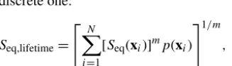
Seq,lifetime=



 

Z

X∈R9

Seq(X)mf(X)dX



 

1/m

, (5)

where f(X) is the joint distribution of the multidimen-sional vector of input variables X. With the above defini-tion, Seq,lifetime is a function of the expected value of the

(7)

discrete one:

Seq,lifetime=

" _N X

i=1

[Seq(xi)]mp(xi) #1/m

, (6)

wherexi, i=1. . .N, is theith realization ofXout ofNtotal

realizations, andp(xi) is the relative, discretized probability

of xi, which is derived by weighting the joint pdf values of

X so that they satisfy the condition PN

i=1p(xi)=1. For a

standard MC simulation, each realization is considered to be equally likely, andp(xi)=1/N.

3.3 Uncertainty estimation and confidence intervals With the present problem of evaluating the uncertainty in aeroelastic simulations – for any specific combination of en-vironmental conditions,xi – there will be uncertainty in the

resulting DELs,Seq(xi). Part of this uncertainty is statistical

by nature and is caused by realization-to-realization varia-tions in the turbulent wind fields used as input to the load simulations. This uncertainty is normally taken into account by carrying out load simulations with multiple realizations (seeds) of turbulence inputs.

Confidence intervals (CIs) reflecting such an uncertainty can be determined in a straightforward way using the boot-strapping technique (Efron, 1979). Its main advantage is ro-bustness and no necessity for assuming a statistical distri-bution of the uncertain variable. With this approach, each function realization is given an integer index, e.g., from 1 toNforNfunction realizations. Then, a “bootstrap” sample is created by generating random integers from 1 toN, and, for each random integer, assigning the original sample point with the corresponding index, as part of the new bootstrap sample. Since the generation of random integers allows for number repetitions, the bootstrap sample will in most cases differ from the original sample. To obtain a measure of the uncertainty in the original sample, a large number of boot-strap samples are drawn, and the resultant quantity of inter-est (e.g., the lifetime fatigue load) is computed for each of them. Then, the empirical distribution of the set of outcomes is used to define the CIs. IfMbootstrap samples have been drawn, andR is the set of outcomes ranked by value in as-cending order, then the (CI) bounds for a confidence levelc`

are

n CI−_S

eq,lifetime(c`), CI +

Seq,lifetime(c`)

o

=R[c`M/2], R[(1−c`/2)M] , (7)

where the square brackets[x]indicate the integer part ofx, and R[x] means the value in R with rank equal to [x]. In

the present study, bootstrapping is applied by generating in-dependent bootstrap samples each with a size equal to the entire data set. Both the sample points and the turbulence seed numbers are shuffled, meaning that the resulting CIs should account for both the statistical uncertainty due to a

finite number of samples, and the uncertainty due to seed-to-seed variation. Note that these two uncertainty types are the only ones assumed for the CIs; reducing the CI by creating a large number of model realizations does not eliminate other model uncertainties, nor does it remove uncertainties in the input variables.

4 Load mapping functions

In this section we present five different approaches that can be used to map loads from a high-fidelity database to inte-grated site-specific design loads:

1. importance sampling,

2. nearest-neighbor interpolation,

3. polynomial chaos expansion,

4. universal Kriging, and

5. quadratic response surface.

The first two methodologies carry out a direct numeri-cal integration over the high-fidelity database presented in Sect. 2.5, while the latter three are machine learning models that are trained using the same database. Despite the different nature of the functions, they serve the same purpose and for brevity we will refer to all of them as “surrogate models”.

4.1 Importance sampling

Figure 2 shows the distributions of the first six input variables from our high-fidelity database (Sect. 2.5), along with the site-specific distributions for reference site 0 (see Table 5 for site list).

One of the simplest and most straightforward (but not nec-essarily most precise) ways of carrying out the integrations needed to obtain predicted statistics is to use importance sampling (IS), where probability weights are applied on each of the database sample points (Ditlevsen and Madsen, 1996). The IS method and various modifications of it are commonly used in wind-energy-related applications (e.g., Choe et al., 2015; Graf et al., 2018). In the classical definition of IS, the integration (importance sampling) function for determining the expected value of a functiong(X) is given by

E[g(X)] =

1

N N X

i=1

g(X)f(Xi)

h(Xi)

, (8)

where in our application

– i=1. . .Nis the sample point number;

– Xi = [x1,i, x2,i, . . ., x9,i]is a 9-component vector array

(8)

– f(Xi)=f(x1,i)·f(x2,i|x1,i)·. . .·f(x9,i|x8,i, . . ., x1,i) is

the joint pdf of sample point i according to the site-specificprobability distribution; and

– h(Xi)=h(x1,i)·h(x2,i|h1,i)·. . .·h(x9,i|x8,i, . . ., x1,i) is

the joint pdf of sample pointiaccording to thegeneric

probability distribution used to generate the database for the nine variables.

Based on the above, it is clear that only points in the database that also have a high probability of occurrence in the site-specific distribution will have a significant contribution to the lifetime load estimate. This could be considered as a non-standard application of the IS approach, because typically the IS sample distribution is chosen to maximize the probability density of the integrand. In the present case, this objective can be satisfied only approximately, and only in cases where the number of IS samples is smaller than the total number of database samples (NIS< N). Under these conditions, the

importance sampling weights (f(Xi)/ h(Xi) from Eq. 8) can

be evaluated for all points in the database. However, the ap-proach adopted in the present paper is to include only theNIS

points with the highest weights (as shown in Sect. 6.2).

4.2 Multi-dimensional interpolation

Estimating an expected function value with a true mul-tidimensional interpolation from the high-fidelity database would require finding a set of neighboring points that form a convex polygon. For problem dimensions higher than 3, this is quite challenging due to the nonstructured sample dis-tribution. However, it is much easier to find a more crude approximation by simply finding the database point closest to the function evaluation point in a nearest-neighbor ap-proach. This is similar to the table look-up technique of-ten used with structured grids; the denser the distribution of the sample points is, the closer will the results be to an ac-tual MC simulation. Finding the nearest neighbor to a func-tion evaluafunc-tion point requires determining the distances be-tween this point and the rest of the points in the sample space. This is done most consistently in a normalized space, i.e., where the input variables have equal scaling. The cu-mulative distribution function (CDF) of the variables is an example of such a space, as all CDFs have the same range of (0,1). Thus, the normalized distance between a new evalua-tion point and an existing sample is computed as the vector norm of the (e.g., 9-dimensional vector) differences between the marginal CDF for the two points:

|x| = √

DT_D_, ₍₉₎

where D=Y− ˆY is the difference between the current evaluation point Y and the existing sam-ple points in the reference database, Y. The vectorˆ YT= [F1(X1), F2(X2|X1), . . ., Fn(Xn|X1, . . ., Xn−1)]

con-sists of the marginal CDFs of the input variables X as obtained using a Rosenblatt transformation.

Since some of the input variables may have significantly bigger influence on the result than other variables, it may be useful to weight the CDF of different variables according to their importance (e.g., by making the weights proportional to the variable sensitivity indices; see Sect. 4.6).

4.3 Polynomial chaos expansion

Polynomial chaos expansion (PCE) is a popular method for approximating a stochastic function of multiple random vari-ables using an orthogonal polynomial basis. For the present problem, using a Wiener–Askey generalized PCE (Xiu and Karniadakis, 2002) employing Legendre polynomials is con-sidered most suitable for any (scaled) variableξ∈ [−1,1]. Because Legendre polynomialsPn(ξ) are orthogonal with

re-spect to a uniform probability measure, the PCE can conve-niently be applied to the CDFs of the variablesX that are defined in the interval[0,1]. Then

ξi=2F(Xi)−1, (10)

whereF(Xi) is the cumulative distribution function of a

vari-ableXi∈X,i=1, . . ., M. The Legendre polynomial

coeffi-cients can be generated using the recurrence relation

(n+1)Pn+1(ξ)=(2n+1)ξ Pn(ξ)−nPn−1(ξ), (11)

where the first two entries,P0(ξ)=1 and P1(ξ)=ξ, serve

for initialization. The aim of using PCE is to represent a scalar quantityS=g(X) in terms of a truncated sequence eS(X)+ε, where ε is a zero-mean residual term. With this definition, the multivariate generalized PCE of dimensionM

and maximum degreepis given by

eS(ξ)= Np−1

X

j=0

Sj9γ,j(ξ); (12)

here9γ are multivariate orthogonal polynomials composed of the product of univariate polynomials having (nonnegative integer) orders defined by the vectorγ= [γ1, . . ., γM], with

the total of orders being constrained by the degree:PM i=1γi≤ p. The unknown coefficientsSj∈S= [S1, . . ., SNp]need to

be determined, andξ= [ξ1, . . .ξM]are functions ofXas

fined in Eq. (10). Training the PCE model amounts to de-termining the vector of coefficients,S. For a more detailed explanation of the training process, as well as the basic PCE theory, the reader is referred to Appendix A (and further to Xiu and Karniadakis, 2002; Sudret, 2008, for yet more de-tail).

4.4 Universal Kriging with polynomial chaos basis functions

(9)

vari-able follows a Gaussian process. A Kriging model is de-scribed (Sacks et al., 1989) by

Y(X)=f(X)Tβ+Z(X), (13)

where forNevaluation samples and anM-dimensional prob-lem, Xrepresents an M×N matrix of input variables and

Y(X) is the output vector. The termf(X)Tβis the mean value of the Gaussian process (a.k.a. the “trend”) represented as a set of basis functionsf(X)= [f1(X), . . ., fP(X)]and

regres-sion coefficients β= [β1, . . ., βP], whereas Z(X) is a zero-mean stationary Gaussian process. The (joint) probability distribution of the Gaussian process is characterized by its covariance; for two distinct “points”XandWin the sample domain the covariance is defined as

V(W,X)=σ2R(W,X,θ), (14)

whereσ2is the overall process variance that is assumed to be constant, andR(W,X,θ) is the correlation betweenZ(X) andZ(W). The hyperparametersθdefine the correlation be-havior, in terms of correlation length scale(s) for example. Since the mean and variance of the Gaussian field can be expressed as functions ofθ (this is shown in details in Ap-pendix A), the calibration of the Kriging model amounts to determining the trend coefficients and obtaining an optimal solution forθ.

The functional form of the mean fieldf(X)Tβis identical to the generalized PCE defined in Eq. (A8), meaning that the PCE is a possible candidate model for the mean in a Kriging interpolation. We adopt this approach and define the Kriging mean as a PCE with properties as described in Sect. 4.3. A suitable approach for tuning the Gaussian field statistics is to find the values ofβ,σ2andθthat maximize the likelihood of the training set variablesY,i.e., minimize the model er-ror in a least-squares sense (Lataniotis et al., 2015). This is described in Appendix A.

The main practical difference between regression- or expansion-type models such as regular PCE and the Kriging approach ishowthe training sample is used in the model: in pure regression-based approaches the training sample is used to only calibrate the regression coefficients, while in Kriging (and in other interpolation techniques) the training sample is retained and used in every new model evaluation. As a result the Kriging model may have an advantage in accuracy, since the model error tends to zero in the vicinity of the training points; however, this comes at the expense of an increase in the computational demands for new model evaluations. For a Kriging model, a gain in accuracy over the model represented by the trend function will only materialize in problems where there is a noticeable correlation between the residual values at different training points. In a situation where the model er-ror is independent from point to point (e.g., in the case when the error is only due to seed-to-seed variations in turbulence) the inferred correlation length will tend to zero and the Krig-ing estimator will be represented by the trend function alone.

4.5 Quadratic response surface

A quadratic-polynomial response surface (RS) method based on central composite design (CCD) is a reduced-order model which, among other applications, has been used for wind tur-bine load prediction (Toft et al., 2016). The procedure in-volves fitting a quadratic polynomial regression (“response surface”) to a normalized space of i.i.d. variables, which are derived from the physical variables using an isoprobabilis-tic transformation – such as the Rosenblatt transformation given in Eqs. (1) and (2). The design points used for cali-brating the response surface ink dimensions form a com-bination of a central point, axial points a distance of

√

kin each dimension, and a 2k “factorial design” set where there are two levels (points) per variable dimension located at unit distance from the origin; this is shown in Fig. 3 for the case of k=2 variables (dimensions). Due to the structured de-sign grid required, it is not possible to use this approach with the sample points from the high-fidelity database described in Sect. 2; therefore, we implement the procedure using an additional set of simulations. The low order of the response surface also prohibits full characterization of the highly non-linear turbine response as a function of mean wind speed us-ing a sus-ingle response surface. Therefore, multiple response surfaces are calibrated for wind speeds from 4 to 25 m s−1 in 1 m s−1steps. This approach may in principle be extended to include additional variables such as turbulence (σu), but

doing so will reduce the practicality of the procedure as it will require multidimensional interpolation between a large number of models and the uncertainty may increase. How-ever, due to the exponential increase in the number of design points with increasing problem dimension, it is not practi-cal to fit a response surface covering all nine variables con-sidered. Instead, we choose to replace three of the variables with relatively low importance (yaw, tilt, and air density) with their mean values. The result is a 6-dimensional prob-lem consisting of 22 different 5-dimensional response sur-faces, which require 22·(1+2·5+25)=946 design points in total. Analogous to the high-fidelity database, 8 h of sim-ulations are carried out for characterizing each design point. The polynomial coefficients of the response surface are then defined using least-squares regression with the same closed-form solution defined by Eq. (A8). For any sample pointp

in the CCD, the corresponding row in the design matrix is defined as

9p= h

{1}, {U1, . . .Un}, {U12, . . .Un2},

Ui·Uj, i=1. . .n, j=1. . .(i−1) i

, (15)

(10)

u₁

-1.5 -1 -0.5 0 0.5 1 1.5

u2

-1.5 -1 -0.5 0 0.5 1 1.5

Figure 3.Example of a rotatable central composite design (CCD) in a 2-dimensional standard normal space[u1, u2]. The CCD

con-sists of a central point, a 2k “factorial design” with 2 levels and

k=2 dimensions, and axial points at distanceu= √

2, meaning that all the outer points lie on a circle.

4.6 Sensitivity indices

We use the global Sobol indices, Sobol (2001), for evaluating the sensitivity of the response with respect to input variables. Having trained a surrogate model, the total Sobol indices can be computed efficiently by carrying out a MC simulation on the surrogate. For number of dimensions equal to M (e.g.,

M=9 in the present study) and forN (quasi) MC samples the required experimental design represents anN×2M ma-trix. This is divided into twoN×Mmatrices,AandB. Then, for each dimension i,i=1. . .M, a third matrixABi is

cre-ated by taking theith column ofABi equal to theith column

fromB, and all other columns taken fromA. The load sur-rogate is then evaluated for all three matrices, resulting in three model estimates:f(A),f(B), andf(ABi). By

repeat-ing this for i=1. . .M, simulation-based Sobol’ sensitivity indices can be estimated as

SUi=

1

N N X

j=1

f(B)j f(ABi)j−f(B)j, (16)

wherej =1. . .N is the row index in the design matricesA, B, andABi (Saltelli et al., 2008). For the problem discussed

in the present study, it was sufficient to use approximately 500 MC samples per variable dimension in order to compute the total Sobol indices.

4.7 Model reduction

For any polynomial-based regression model that includes de-pendence between variables, the problem grows steeply in size when the number of dimensions,M, and the maximum polynomial order,p, increase. In such situations, it may be

desirable to limit the number of active coefficients by car-rying out a least absolute shrinkage and selection operator (LASSO) regression (Tibshirani, 1996), which regularizes the regression by penalizing the sum of the absolute value of regression coefficients. For a PCE model, the objective function using a LASSO regularization is

S=min   

 

1 2Ne

Ne

X

i=1



g(ξ

(i)₎₋

Np−1

X

j=0

Sj9γ,j(ξ(i)) 



2

+λ Np−1

X

j=0

|Sj|  



, (17)

whereλis a positive regularization parameter; larger values ofλincrease the penalty and reduce the absolute sum of the regression coefficients, whileλ=0 is equivalent to ordinary least-squares regression. In the present study, the LASSO regularization is used on the PCE-based models to reduce the number of coefficients.

One useful corollary of the orthogonality in the PCE poly-nomial basis is that the contribution of each individual term to the total variance of the expansion (i.e., the individual Sobol indices) can be easily computed based on the coeffi-cient values (see Appendix A). This property can be used for eliminating polynomials that do not significantly contribute to the variance of the output, thus achieving a sparse, more computationally efficient, reduced model. By combining the variance truncation and the LASSO regression technique in Eq. (17), a model reduction of an order of magnitude or more can be achieved. For example, for the 9-dimensional PCE of order 6 discussed in Sect. 5.3, using LASSO regularization parameterλ=1 and retaining the polynomials that have a total variance contribution of 99.5 % resulted in a reduction of the number of polynomials from 5005 to about 200.

5 Model training and performance

5.1 Model convergence

We assess the convergence of PCE by calculating the nor-malized root-mean-square error (NRMSE) between a set of observed quantities (i.e., DELs from simulations) y=

g(X(i)), i=1. . .N, and the PCE predictions,_ey=eS(X(i)), i= 1. . .N, over the same set ofN sample pointsX(i) from the training sample defined in Sect. 2:

εNRMS=

1

E[y] v u u u t

N P

i=1

(_eyi−yi)2

N , (18)

(11)

8

Hours simulation per sample

6 Convergence of site-specific DEL

estimated with PCE, order 6, 6 dimensions

4 2 0 4000 Number of training sample

s 3000 2000

1000 0.1 0.2 0.3 0.4 0.5

Normalized root mean square error

Figure 4.Convergence of a PCE of dimension 6 and order 6, as a function of number of collocation points and hours of simulation per collocation point. Thezaxis represents the NRMSE obtained from the difference between 500 site-specific quasi-MC samples of blade root flapwise DEL for reference site 0, and the corresponding predictions from PCE.

samples used to train the PCE, and the hours of load simula-tions (i.e., number of seeds) used for each sample point. The NRMSE shown in Fig. 4 is calculated based on a set of 500 quasi-MC points sampled from the joint pdf of reference site 0, and represents the difference in blade root flapwise DEL observed in each of the 500 points vs. the DEL predicted by a PC expansion trained on a selection of points from the high-fidelity database described in Sect. 2. Each of the quasi-MC samples is the mean from 48 turbulent 10 min simulations. To mimic the seed-to-seed uncertainty, each of the PCE predic-tions is also evaluated as the mean of 48 normally distributed random realizations, with mean and standard deviation pre-scribed by the PCE model for mean and standard deviation of the blade flapwise DEL, respectively.

Figure 4 illustrates a general tendency that using a few thousand training samples leads to convergence of the val-ues of the PC coefficients, and the remaining uncertainty is due to seed-to-seed variations and due to the order of the PCE being lower than what is required for providing an ex-act solution at each sample point. Using longer simulations per sample point does not lead to further reduction in the statistical uncertainty due to seed-to-seed variations – with 4000 training samples, the NRMSE for 1 h simulation per sample is almost identical to the error with 8 h simulation per sample. The explanation for this observation is that the seed-to-seed variation introduces an uncertainty not only be-tween different simulations within the same sampling point but also between different sampling points. This uncertainty materializes as an additional variance which is not explained by the smooth PCE surface. Further increase in the number

Number of database samples used

0 2000 4000 6000 8000 10 000

Normalized blade root M

x

lifetime DEL

0.5 1 1.5

Site-specific reference, mean

Site-specific reference, lower 95 % CI bound Site-specific reference, upper 95 % CI bound Importance sampling from database, mean

Importance sampling from database, lower 95 % CI bound Importance sampling from database, upper 95 % CI bound

Figure 5.Convergence of an importance sampling (IS) calculation of the blade root moment from the high-fidelity database towards site-specific lifetime fatigue loads for reference site 0 (Table 5).

of training points or simulation length will only reduce this statistical uncertainty, but will not contribute significantly to changes in the model predictions as the flexibility of the model is limited by the maximum polynomial order. There-fore, the model performance achieved under these conditions can be considered near to the best possible for the given PCE order and number of dimensions. However, it should be noted that the number of training points required for such conver-gence will differ according to the order and dimension of the PCE, and higher order and more dimensions will require more than the approximately 3000 points that seem sufficient for a PCE of order 6 with six dimensions, as shown in Fig. 4. The IS procedure has relatively slow convergence com-pared to, for example, a quasi-MC simulation. Figure 5 shows an example of the convergence of an IS integration for reference site 0, based on computing the target (site-specific) distribution weights for all 104 points in a reference high-fidelity database. The CIs are obtained by bootstrapping.

(12)

tur-Table 2.Normalized root mean square error characterizing the difference between aeroelastic simulations and reduced-order models. Load channel abbreviations are the following: TB: tower base; TT: tower top; MS: main shaft; BR: blade root. Loading directions consist ofMx: fore-aft (flapwise) bending,My: side-side (edgewise) bending, andMz: torsion.

Normalized rms error – site 0

Prediction model Load channels

TBMx TBMy TTMx TTMy TTMz MSMz BRMx BRMy

Quadratic RS 0.0452 0.1404 0.1981 0.2612 0.0644 0.2280 0.1504 0.0098 PC expansion 0.0362 0.0955 0.1019 0.2089 0.0362 0.1530 0.0620 0.0084

Kriging 0.0334 0.0706 0.0837 0.1761 0.0368 0.1072 0.0519 0.0083

Table 3.PCE-based Sobol sensitivity indices for the high-fidelity load database variable ranges.

Fatigue load sensitivity indices

Load channel Variables

U σu α L 0 1ϕh ϕh ϕv ρ

Tower base fore-aft momentMx 0.42 0.65 0.01 0.03 0.02 0.01 0.00 0.00 0.01 Tower base side-side momentMy 0.62 0.42 0.05 0.04 0.04 0.02 0.02 0.02 0.02 Blade root flapwise momentMx 0.20 0.64 0.19 0.02 0.01 0.00 0.01 0.00 0.02 Blade root edgewise momentMy 0.22 0.54 0.25 0.05 0.03 0.01 0.01 0.03 0.01 Tower top yaw momentMz 0.14 0.85 0.00 0.02 0.01 0.00 0.00 0.00 0.01

Main shaft torsionMz 0.48 0.53 0.01 0.06 0.01 0.01 0.01 0.01 0.01

bulence seeds simulated with these conditions. The values of the NRMSE for site 0 for Kriging, RS, and PCE-based load predictions are listed in Table 2. In addition, Fig. 6 presents a one-to-one comparison where for a set of 200 sample points, the load estimates from the site-specific MC simulations are compared against the corresponding surrogate model predic-tions in terms ofy−yplots.

The RMS error analysis reveals a slightly different picture. In contrast to the lifetime DEL where the Kriging, PCE, and RS methods showed very similar results, the RMS error of the quadratic RS is for some channels about twice the RMS error of the other two approaches.

5.3 Variable sensitivities

As described earlier in Sect. 4.6, we consider variable sensi-tivities (i.e., the influence of input variables on the variance of the outcome) in terms of Sobol indices. By definition the Sobol indices will be dependent on the variance of input vari-ables, meaning that for one and the same model, the Sobol indices will be varying under different (site-specific) input variable distributions. Taking this into account, we evaluate the Sobol indices for the two types of joint variable distri-butions used in this study – (1) a site-specific distribution, and (2) the joint distribution used to generate the database with high-fidelity load simulations. The total Sobol indices for the high-fidelity load database variable range are com-puted directly from the PCE fitted to the database by

eval-uating the variance contributions from the expansion coeffi-cients (see Appendix A) and are listed in Table 3. The in-dices for the site-specific distribution corresponding to ref-erence site 0 are computed using the method based on MC simulations described in Sect. 4.6, as direct PCE indices are not available for this sample distribution. The resulting to-tal Sobol indices for the six variables available at site 0 are listed in Table 4. The two tables show similar results – the mean wind speed and the turbulence are the most important factors affecting both fatigue and extreme loads. Two other variables that show a smaller but still noticeable influence are the wind shear,α, and the Mann model turbulence length scale,L. The effect of wind shear is pronounced mainly for blade root loads that can be explained by the rotation of the blades, which, if subjected to wind shear, will experience cyclic changes in wind velocity. The effect of Mann model

0, veer, yaw, tilt, and air density within the chosen variable ranges seems to be minimal, especially for fatigue loads.

6 Site-specific calculations

6.1 Reference sites

(13)

MC sample means

0 0.2 0.4 0.6 0.8 1

RS prediction means

0 0.2 0.4 0.6 0.8 1

RS vs. MC

MC sample means

0 0.2 0.4 0.6 0.8 1

PCE prediction means

0 0.2 0.4 0.6 0.8 1

PCE vs. MC

MC sample means

0 0.2 0.4 0.6 0.8 1

KM prediction means

0 0.2 0.4 0.6 0.8 1

KM vs. MC

Figure 6.y−yplots comparing the blade root flapwise 1 Hz damage-equivalent load (DEL) predictions for three load surrogate models – quadratic Response Surface, Polynomial Chaos expansion, and Kriging model, compared against site-specific Monte Carlo (MC) simulation. Thexaxis represents the loads obtained using site-specific MC simulations for reference site 0, and theyaxis represents the mean 1 Hz-equivalent load estimated for the same sample points using a surrogate model. All values are normalized with the maximum Hz-equivalent load attained from the site-specific Monte Carlo (MC) simulation.

Table 4. Site-specific Sobol sensitivity indices derived for site 0 using MC simulation from a PCE.

Fatigue load sensitivity indices

Load channel Variables

U σu α L 0

Tower base fore-aft momentMx 0.08 1.32 0.07 0.18 0.09

Tower base side-side momentMy 0.90 0.09 0.07 0.23 0.13

Blade root flapwise momentMx 0.42 0.38 0.05 0.01 0.01

Blade root edgewise momentMy 0.43 0.18 0.26 0.22 0.11

Tower top yaw momentMz 0.23 0.53 0.01 0.08 0.01

Main shaft torsionMz 0.47 0.36 0.06 0.03 0.07

database. In order to show a realistic example of situations where a site-specific load estimation is necessary, the major-ity of the virtual sites chosen are characterized with condi-tions that slightly exceed the standard condicondi-tions specified by a certain type-certification class. Exceptions are site 0, which has the most measured variables available and is there-fore chosen as a primary reference site, and the virtual “sites” representing standard IEC class conditions. The IEC classes are included as test sites as they are described by only one in-dependent variable (mean wind speed). They are useful test conditions as it may be challenging to correctly predict loads as a function of only one variable using a model based on up to nine random variables. The list of test sites is given in Table 5.

Site 0 (also referred to as the reference site) is located at the Nørrekær Enge wind farm in northern Denmark (Borrac-cino et al., 2017), over flat, open agricultural terrain. Site 1 is a flat-terrain near-coastal site at the National Centre for Wind Turbines at Høvsøre, Denmark (Peña et al., 2016). Sites 2 to 4 are based on the wind conditions measured at the Østerild Wind Turbine Test Field, which is located in a large forest plantation in northwestern Denmark (Hansen et al., 2014).

Due to the forested surroundings of the site, the flow con-ditions are more complex than those in Nørrekær Enge and Høvsøre. By applying different filtering according to wind direction, three virtual site climates are generated and con-sidered as sites 2–4.

Sites 5 and 6 are located at NREL’s National Wind Tech-nology Center (NWTC), near the base of the Rocky Moun-tain foothills just south of Boulder, Colorado (Clifton et al., 2013). Similar to Østerild, directional filtering is applied to the NTWC data to split it into two virtual sites – accounting for the different conditions and wind climates from the two ranges of directions considered.

For each site, the joint distributions of all variables are de-fined in terms of conditional dependencies, and generating simulations of site-specific conditions is carried out using the Rosenblatt transformation, Eq. (1). The conditional depen-dencies are described in terms of functional relationships be-tween the governing variable and the distribution parameters of the dependent variable, e.g., the mean and standard devi-ation of the turbulence are modeled as linearly dependent on the wind speed as recommended by the IEC 61400-1 (ed. 3, 2005) standard. The wind shear exponent is dependent on the mean wind speed and on the turbulence, and the distribution parameters ofαare defined by the relationship (Kelly et al., 2014; Dimitrov et al., 2015)

µα|Ic,u=αref+

Ic,ref−Ic(U)

Ic(U)·cα

, (19)

σα=1/U,

whereµα and σα are the mean and standard deviation of α, respectively;Ic(U)=(σu/U|F(σu)=Q) is a

character-istic turbulence intensity based on a turbulence quantileQ, as a function of the wind speed U. Here Ic,ref=Ic(U=

15 m s−1) is the reference characteristic turbulence intensity atU=15m s−1andαref=α|(Ic=Ic,ref, U=15m s−1) is a

(14)

Table 5.Reference virtual sites used for validation of the site-specific load estimation methods.

Site no. Location Terrain Specific condition Variables included MC sample size

0 Denmark Flat agricultural – U, σu, α, L, 0, 1ϕ 492

1 Denmark Flat agricultural IIIC exceedance U, σu, α 823

2 Denmark Forested IIIB exceedance U, σu, α 884

3 Denmark Forested IA exceedance U, σu, α 949

4 Denmark Forested IIA exceedance U, σu, α 871

5 Colorado, USA Mountain foothills Low-wind U, σu, α 657

6 Colorado, USA Mountain foothills Low-wind U, σu, α 853

IEC IA, NTM – – Standard reference class U 22

IEC IIB, NTM – – Standard reference class U 22

IEC IIIC, NTM – – Standard reference class U 22

IEC IIB, ETM – – Standard reference class U 22

determined constant. Since the turbulence quantities Ic(u)

andIc,refare defined by the conditional relationship between

wind speed and turbulence, the only site-specific parameters required for characterizing the wind shear are αref andcα.

For each of the physical sites, the wind speed, turbulence and wind shear distribution parameters are defined based on anemometer measurements at the sites. The results are listed in Table 6. In addition, high-frequency 3-D sonic measure-ments were available at site 0 for the entire measurement pe-riod, which allowed for estimating Mann turbulence model parameters using the approach described in Dimitrov et al. (2017).

With this procedure, 1000 quasi-MC samples of the en-vironmental conditions at each site are generated from the respective joint distribution. All realizations where the wind speed is between the DTU 10 MW wind turbine cut-in and cut-out wind speed are fed as input to load simulations. The actual number of load simulations for each site are given in Table 6. Similarly to the load database simulations, eight sim-ulations with 1 h duration are carried out at each site-specific MC sample point. The resulting reference lifetime equivalent loads are then defined by applying Eq. (6) on the MC simu-lations using equal weightsp(Xi)=1/N, while the

uncer-tainty in the lifetime loads is estimated using bootstrapping on the entire MC sample.

6.2 Lifetime fatigue loads

The lifetime damage-equivalent loads (DELs) are computed for all reference sites in Table 5, using the five load surro-gate models defined above: (1) quadratic response surface; (2) polynomial chaos expansion, (3) importance sampling, (4) nearest-neighbor interpolation, and (5) Kriging with the mean defined by polynomial chaos basis functions. Methods 2–5 are based on data from the high-fidelity load database described in Sect. 2. In addition to the surrogate model com-putations, a full MC reference simulation is carried out for each validation site. The load predictions with the MC ap-proach are obtained by carrying out Hawc2 aeroelastic

Site MC

Quadratic RS

PC expansion

Importance Sampling

Interpolation Kriging

Normalized lifetime DEL

0.8 0.9 1 1.1 1.2

Main shaft torsion M_z lifetime DEL: mean and 95 % CI estimates, reference site #0

Mean from site-specific MC simulation 95 % confidence bounds from site-specific MC

O4

O6

Figure 7. Comparison of predictions of the lifetime

damage-equivalent loads (DELs) for six different estimation approaches. All values are normalized with respect to the mean estimate from a site-specific Monte Carlo (MC) simulation, and the error bars represent the bounds of the 95 % confidence intervals (CIs). Results from two PCEs are shown: the blue bar corresponds to the output of a fourth-order PCE, while the black bar corresponds to a sixth-fourth-order PCE.

ulations on the same DTU 10 MW reference wind turbine model used for training the load surrogate models. A to-tal ofNMC=1000 quasi-MC samples are drawn from the

(15)

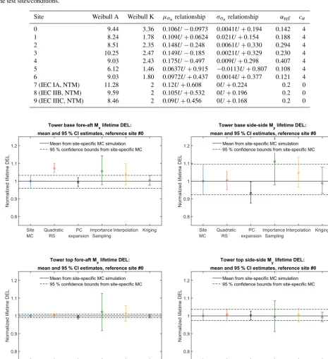
Table 6.Parameters defining the conditional distribution relationships used in computing joint distributions of the environmental conditions for the test sites/conditions.

Site Weibull A Weibull K µσurelationship σσurelationship αref cα

0 9.44 3.36 0.106U−0.0973 0.0041U+0.194 0.142 4

1 8.24 1.78 0.109U+0.0624 0.021U+0.154 0.188 4

2 8.51 2.35 0.148U−0.248 0.0061U+0.330 0.294 4

3 10.25 2.47 0.149U−0.185 0.0021U+0.329 0.230 4

4 9.03 2.43 0.175U−0.497 0.009U+0.298 0.407 4

5 6.12 1.46 0.0637U+0.915 −0.0113U+0.807 0.108 4

6 9.03 1.80 0.0972U+0.437 0.0014U+0.377 0.121 4

7 (IEC IA, NTM) 11.28 2 0.12U+0.608 0U+0.224 0.2 0

8 (IEC IIB, NTM) 9.59 2 0.105U+0.532 0U+0.196 0.2 0

9 (IEC IIIC, NTM) 8.46 2 0.09U+0.456 0U+0.168 0.2 0

Site MC

Quadratic RS

PC expansion

Importance Sampling

0.8 0.9 1 1.1 1.2

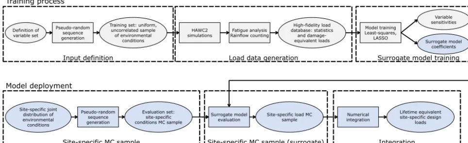
Tower base fore-aft M_x lifetime DEL: mean and 95 % CI estimates, reference site #0

Site MC

Quadratic RS

PC expansion

Importance Sampling

0.8 0.9 1 1.1 1.2

Tower base side-side M_y lifetime DEL: mean and 95 % CI estimates, reference site #0

Site MC

Quadratic RS

PC expansion

Importance Sampling

0.8 0.9 1 1.1 1.2

Tower top fore-aft M

x lifetime DEL: mean and 95 % CI estimates, reference site #0

Site MC

Quadratic RS

PC expansion

Importance Sampling

0.8 0.9 1 1.1 1.2

Tower top side-side M

y lifetime DEL: mean and 95 % CI estimates, reference site #0

Figure 8.Comparison of predictions of the lifetime damage-equivalent loads (DELs) for six different estimation approaches. All values are normalized with respect to the mean estimate from a site-specific Monte Carlo simulation.

reference MC simulations. The load predictions with impor-tance sampling are based on the probability-weighted con-tributions from the samples in a high-fidelity load database. For each site-specific distribution, the database samples are ordered according to their weights, and only a number of points, NIS, with the highest weights are used in the

esti-mation. For the sake of easier comparison between different methods, it is chosen thatNIS=NMC. Based on

(16)

Site MC

Quadratic RS

PC expansion

Importance Sampling

0.8 0.9 1 1.1 1.2

Yaw moment M_z lifetime DEL: mean and 95 % CI estimates, reference site #0

Site MC

Quadratic RS

PC expansion

Importance Sampling

0.8 0.9 1 1.1 1.2

Main shaft torsion M_z lifetime DEL: mean and 95 % CI estimates, reference site #0

Site MC

Quadratic RS

PC expansion

Importance Sampling

0.8 0.9 1 1.1 1.2

Blade root flapwise M_x lifetime DEL: mean and 95 % CI estimates, reference site #0

Site MC

Quadratic RS

PC expansion

Importance Sampling

0.8 0.9 1 1.1 1.2

Blade root edgewise M_y lifetime DEL: mean and 95 % CI estimates, reference site #0

Figure 9.Comparison of predictions of the lifetime damage-equivalent loads (DELs) for six different estimation approaches. All values are normalized with respect to the mean estimate from a site-specific Monte Carlo simulation.

diction of main shaft torsion loads using order 4 and order 6 PC expansion are compared against other methods, and the order 4 calculation shows a significant bias. Therefore, the PC expansion used for reporting the results in this section is based on the same 6-dimensional variable input used with the quadratic response surface, and has a maximum order of 6. For evaluating CIs from the reduced-order models (Krig-ing, PCE, and quadratic response surface), two reduced-order models of each type are calibrated – one for the mean val-ues, and the other for the standard deviations. This allows for generating a number of realizations for each sampled com-bination of input variables, and subsequently computing CIs by bootstrapping (Eq. 7). In this way, the bootstrapping is done simultaneously for a random sample of the input vari-ables and the random seed-to-seed variations within each sample. As a result, the obtained CI reflects the combina-tion of seed-to-seed uncertainty and the uncertainty due to a finite number of samples from the distribution of the in-put variables. This approach also allows for consistency with the importance sampling and nearest-neighbor interpolation techniques, where the same bootstrapping approach is used.

Since the lifetime fatigue load is in essence an integrated quantity subject to the law of large numbers, the uncertainty in computations based on a random sample of sizeNwill be proportional to 1/

√

N. Comparing uncertainties and CIs as defined in Sect. 3.3 will therefore only be meaningful when approximately the same number of samples is used for all calculation methods. This approach is used for generating Figs. 8 and 9, where the performance of all site-specific load estimation methods is compared for reference site 0, for eight load channels in total, with the number of samples as listed in Table 8. Figure 8 shows results for tower base and tower top fore-aft and side-side bending moments, and Fig. 9 displays the tower top yaw moment, the main shaft torsion, and blade root flapwise and edgewise bending moments.

(17)

Table 7.Lifetime-equivalent load predictions normalized with respect to MC simulations and averaged over 10 reference sites. Load channel abbreviations are the following: TB: tower base; TT: tower top; MS: main shaft; BR: blade root. Loading directions consist ofMx: fore-aft (flapwise) bending;My: side-side (edgewise) bending; andMz: torsion.

Load channels

TBMx TBMy TTMx TTMy TTMz MSMz BRMx BRMy

Polynomial chaos expansion

Mean 0.966 0.934 0.978 1.000 0.991 1.018 1.003 0.999

SD 0.030 0.014 0.019 0.019 0.018 0.026 0.014 0.002

Universal Kriging

Mean 0.972 0.965 0.989 0.998 0.992 0.993 1.008 1.000

SD 0.033 0.028 0.018 0.019 0.020 0.027 0.015 0.002

Quadratic response surface

Mean 1.034 0.980 0.966 1.032 1.014 1.075 1.021 0.996

SD 0.029 0.027 0.017 0.015 0.012 0.028 0.012 0.003

Importance sampling

Mean 0.859 0.878 0.862 1.102 0.932 1.251 1.100 0.992

SD 0.101 0.088 0.067 0.075 0.063 0.088 0.086 0.007

Nearest-neighbor interpolation

Mean 0.951 0.993 0.951 0.989 0.972 1.066 1.001 0.994

SD 0.081 0.057 0.045 0.064 0.052 0.070 0.044 0.005

Table 8.Model execution times for the lifetime damage-equivalent fatigue load computations for site 0.

Surrogate Training Evaluation Evaluation

model set size set size time

MC – 492 22.7 s

PCE 10 000 492 8.2 s

RS 946 492 2.2 s

IS 10 000 492 4.6 s

NN 10 000 492 4.4 s

Kriging 2048 492 217.6 s

validation sites. The summarized site-specific results for all surrogate-based load estimation methods are shown in Ta-ble 7. In order to compute these values, the load estimates for each site and load channel are normalized to the results obtained with the direct site-specific MC simulations. The values given in Table 7 are averaged over all reference sites. The results for individual sites and load channels are depicted as bar plots in Figs. 10 and 11 for tower load and rotor load channels, respectively. The largest observed errors amount to≈9 % with Kriging,≈10 % for the PCE,≈10 % for the quadratic RS,≈24 % for IS, and∼15–17 % for NN inter-polation. Noticeably, the low wind speed, high turbulence site 5 seems to be the most difficult for prediction – for most load prediction methods this is the site where the largest

er-ror is found. All models except the Kriging also show rel-atively large errors for the IEC class-based sites. That can be attributed to the significantly smaller number of samples used for the IEC-based sites (22 samples where only the wind speed is varied in 1 m s−1steps from 4 to 25 m s−1). As men-tioned above, the statistical uncertainty in the estimation of the lifetime DEL will diminish with increasing number of samples. In addition to this effect, as discussed in Sect. 4.1, the uncertainty in the IS model can increase when the site-specific distribution has fewer dimensions than the model be-cause fewer points from the high-fidelity database will have high probabilities with respect to the site-specific distribu-tion. It can be expected that this effect is strongest for the IEC class-based sites, as for them only a single variable – the wind speed – is considered stochastic.