Earth Syst. Sci. Data, 11, 1129–1152, 2019 https://doi.org/10.5194/essd-11-1129-2019 © Author(s) 2019. This work is distributed under the Creative Commons Attribution 4.0 License.
Simple noise estimates and pseudoproxies
for the last 21 000 years
Oliver Bothe, Sebastian Wagner, and Eduardo Zorita
Institute of Coastal Research, Helmholtz Zentrum Geesthacht, 21502 Geesthacht, Germany Correspondence:Oliver Bothe (ol.bothe@gmail.com)
Received: 3 November 2018 – Discussion started: 9 November 2018 Revised: 29 March 2019 – Accepted: 7 July 2019 – Published: 1 August 2019
Abstract. Climate reconstructions are means to extract the signal from uncertain paleo-observations, so-called proxies. It is essential to evaluate these reconstructions to understand and quantify their uncertainties. Similarly, comparing climate simulations and proxies requires approaches to bridge the temporal and spatial differences between both and to address their specific uncertainties. One way to achieve these two goals is so-called pseu-doproxies. These are surrogate proxy records within the virtual reality of a climate simulation. They in turn depend on an understanding of the uncertainties of the real proxies including the noise characteristics disturb-ing the original environmental signal. Common pseudoproxy approaches so far concentrate on data with high temporal resolution over the last approximately 2000 years. Here we provide a simple but flexible noise model for potentially low-resolution sedimentary climate proxies for temperature on millennial timescales, the code for calculating a set of pseudoproxies from a simulation, and one example of pseudoproxies. The noise model con-siders the influence of other environmental variables, a dependence on the climate state, a bias due to changing seasonality, modifications of the archive (for example bioturbation), potential sampling variability, and a mea-surement error. Model, code, and data allow us to develop new ways of comparing simulation data with proxies on long timescales. Code and data are available at https://doi.org/10.17605/OSF.IO/ZBEHX (Bothe et al., 2018).
1 Introduction
Proxy records and derived reconstructions are our only ob-servationally based information about past climates before the period covered by human observations, that is before we have documentary or instrumental evidence. Climate recon-struction methods statistically process the information in the proxy records to extract the recorded climate signal. How-ever, multiple variables influence the signal recorded, and we are often only interested or able to extract the contribution of one single climatic parameter.
All other imprints of climate are noise with regard to this variable of interest. Furthermore, part of the variability in the proxy records is not caused by the climate but other factors influencing the original generation of the proxy record. Thus, there are climatic and non-climatic noise contributions to the proxy variability. This proxy noise may cause biases and un-certainties in the resulting climate reconstructions. Evaluat-ing the quality and reliability of reconstructions and of proxy
records requires an understanding of the noise in the proxy records. Only this knowledge allows us to obtain reliable es-timates of the errors in reconstructed properties.
Some aspects of statistical climate reconstruction methods can be evaluated in so-called pseudoproxy experiments. In these experiments, the reconstruction methods are mimicked for example in the controlled conditions provided by climate simulations with Earth system models. However, for these tests surrogate proxy records have to be produced, which are compatible with the climate simulated by these models – the pseudoproxies. In testing the reconstruction methods, pseu-doproxies eventually replace the real paleo-observations in the method and the virtual climate of the Earth system simu-lation stands in for the real climate.
an application. The term does not necessarily refer to sub-stitutes for specific proxy records or particular proxy types. That is, the term pseudoproxy does not by itself imply that the modifications of the input data validly represent the un-certainties or characteristics of real-world data. This view of the term pseudoproxy is in line with the past literature (com-pare, for example, Mann and Rutherford, 2002; Osborn and Briffa, 2004; Von Storch et al., 2004; Jones et al., 2009; Gra-ham and Wahl, 2011; Thompson et al., 2011; Lehner et al., 2012; Smerdon, 2012; Hind et al., 2012; Annan and Harg-reaves, 2013; Kurahashi-Nakamura et al., 2014; Steiger and Hakim, 2016). Modifications of the input data may be as sim-ple as adding white or coloured noise or they may invoke more complex forward approaches (for example mechanistic proxy system models; Evans et al., 2013, see below).
Studies of the climate of the past 2000 years regularly use such pseudoproxy approaches mimicking annually resolved proxies such as dendroclimatogical ones. Smerdon (2012) reviews the approach of using pseudoproxy experiments to evaluate reconstruction methods with a focus on the last mil-lennium. Such methods basically originated in the work of Mann and Rutherford (2002) focussing on climate-field re-constructions. The review by Smerdon (2012) emphasizes the essential contribution of pseudoproxy experiments to our understanding of past climates and to evaluating our meth-ods of studying past climates. To date, most studies using pseudoproxies concentrated on the last few millennia. Few studies considered periods further in the past (e.g. Laepple and Huybers, 2013; Dolman and Laepple, 2018; Dee et al., 2018).
For a useful test of reconstruction methods, the pseudo-proxies should be as realistic as possible, with statistical properties similar to the real proxies. This is achieved by con-taminating the climate variables simulated by the Earth sys-tem model with statistical noise with a certain amplitude and statistical characteristics. These properties ideally are based on estimates of a realistic or at least plausible noise to suc-cessfully mimic the behaviour of real-world proxies.
In our understanding there are various approaches to ob-tain such pseudoproxies. These range from most hensive to most simplified. We can try to obtain a compre-hensive representation of a so-called proxy system (Evans et al., 2013) from the environmental influences on a sensor to our measurement and formulate this into a mechanistic forward model of the system of interest. Such models can be very complex or they may concentrate solely on a core set of processes (compare the full and reduced implementa-tions of the Vaganov–Shashkin approach to modelling tree rings presented by Evans et al., 2006; Tolwinski-Ward et al., 2011). That is, the first approach to obtaining pseudoprox-ies is process-based. Other, more reduced approaches poten-tially ignore this mechanistic process understanding and fo-cus on stochastic expressions of the noise that influence our inferences about past climates. Such an approach can try to formulate mathematically tractable expressions for statistical
noise terms, which represent the different processes or effects influencing the stages from the original environmental condi-tions to our final observation (Andrew M. Dolman, personal communication, 2018, Thomas Laepple, personal communi-cation, 2017). Another way of producing pseudoproxies by focussing on stochastic noise expressions uses simple esti-mates of plausible errors. These different approaches can be specific for certain proxy types or very general. They can fo-cus on one stage of the proxy system from the environment to measurement or consider multiple stages.
All these approaches fit into the concept of a proxy system model as described by Evans et al. (2013). The idea of for-ward models to study the behaviour of proxies and proxy sys-tems is not new (e.g. Schmidt, 1999; Tolwinski-Ward et al., 2011; Thompson et al., 2011) but Evans et al. (2013) were the first to clearly delineate the modelling of proxy systems. A proxy system represents the biological, chemical, geologi-cal, and possibly also documentary system that translates en-vironmental influences into an archived state on which re-searchers make observations. We usually refer to these ob-servations when speaking of climate proxies. A proxy system model is a representation of how the proxy system translates the environmental influences into our observations based on our understanding. Evans et al. (2013) present a generalized concept of this modelling approach, which consists of three components. First, a sensor model reacts to the environmen-tal influences. Second, an archive model transforms these sensor recordings into archive units. A third model trans-lates the archive into representations of what we usually ob-serve on an archive. For example, the sensor “tree” records the environmental influences in its archive “wood”, and we can make measurements on this archive in the form of tree ring counts, widths, etc. The full system from recording to observation is the proxy system.
O. Bothe et al.: Noise and pseudoproxies 1131
accumulated a property of a system. This (property of the) system was sensitive to and recorded an environmental pro-cess at some date. From the recording stage to our inference there are multiple sources of error in our inference.
The potential errors include different sources of noise re-lated to laboratory uncertainties like measurement errors and reproducibility, local disturbances, dating uncertainty, time resolution, serial autocorrelation, and all possibly dependent on the overall climate state. Further uncertainty includes habitat preferences, seasonal biases, the variability in the re-lation between sensor and environment, long-term changes in this relation, long-term modifications of the archive, sam-pling variability and samsam-pling disturbances, and not least generally erroneous assumptions on the researcher’s side about the relation between recording sensor and environ-ment, i.e. the calibration relation. A recipe for calculating pseudoproxies may include potential error estimates for not only parts of the assumed proxy system but also the relation between the “observed” data and time, that is the anchoring of the data in time.
Regarding dating/age uncertainty, there are various ap-proaches to dealing with it (e.g. Breitenbach et al., 2012; Carré et al., 2012; Anchukaitis and Tierney, 2013; Comboul et al., 2014; Goswami et al., 2014; Brierley and Rehfeld, 2014; Rehfeld and Kurths, 2014; Kopp et al., 2016; Boers et al., 2017) of which a number try to transfer the dating un-certainty towards the proxy record unun-certainty (e.g. Breiten-bach et al., 2012; Goswami et al., 2014; Boers et al., 2017). Our interest explicitly is to include the uncertainty from the dating in a statistical noise term for a pseudoproxy time se-ries. Therefore, we do not consider Bayesian or Monte Carlo methods but take a simple approach to develop an error term for the uncertainty in the dating. We also do not include ex-plicit age modelling (compare, e.g. Haslett and Parnell, 2008; Blaauw and Christen, 2011; Trachsel and Telford, 2017).
In addition to evaluating reconstruction methods, a plau-sible estimate of noise within the proxies can also assist in comparison studies between model simulations and the proxy records or among different model simulations. This increases our understanding about past climate changes by consolidating information from all available sources, which are proxy records and model simulations. The lack of high-quality observations with small uncertainty is always go-ing to hamper efforts to assess the quality of model simu-lations of past climates. Such comparisons have to rely on the paleo-observations from proxies, and even the highest-quality proxy records have an irreducible amount of uncer-tainty. Most often data–model comparisons take place in the virtual reality of the model and use the modelled variables. In the case of proxies, the comparison is between, for example, a temperature reconstruction and a model. The alternative is to compare both in the proxy space using a proxy representa-tion of the model climate. Pseudoproxies or a recipe how to compute them may be part of an interface between the data on the one side and the model simulations on the other side.
Recent years saw an intensification in the research on for-ward modelling proxies for understanding proxies, testing re-construction methods, and evaluating simulation output (see, for example, Dolman and Laepple, 2018; Dee et al., 2015, 2018; Konecky et al., 2019). Many of these approaches fol-low the concept of considering sensor, archive, and obser-vations as distinct steps in the process. Still, few of these approaches consider transient timescales beyond the late Holocene. Nevertheless, particularly the work by Dolman and Laepple (2018) and also Dee et al. (2018) allows for the calculation of different sedimentary proxies over multi-millennial timescales based on knowledge of certain pro-cesses in the respective proxy systems.
In this paper, we adopt the conceptual subdivisions of Evans et al. (2013) to present a formal but still simple noise-based approach to describe the disturbances masking the sig-nal in proxy records. This approach can also be applied to produce pseudoproxies for timescales longer than the last few millennia, that is proxies with coarser time resolutions than interannual and afflicted by larger degrees of dating un-certainty. Thereby this work extends previous pseudoproxy approaches, which often concentrated on well-dated proxy systems affected by fewer sources of uncertainty.
The following presents a set of assumptions on proxy noise and estimates for some of the mentioned error sources. We further provide pseudoproxies based on these assumptions for the TraCE-21ka simulation (Liu et al., 2009), which cov-ers the last 21 000 years. We concentrate on proxies which are subject to some kind of sedimentary process. Thus, our work appears to be particularly similar to the proxy system model for sedimentary proxies implemented by Dolman and Laepple (2018). Dolman and Laepple (2018) also consider the long timescales since the last glacial maximum and rely on output from the TraCE-21ka simulation for their forward modelling. Both the present paper and Dolman and Laepple (2018) follow the concept outlined by Evans et al. (2013). The main difference between Dolman and Laepple (2018) and the present study is that they provide a simple process-focussed model of the proxy system, whereas we try to pro-vide a simple characterization of the noise in the proxy sys-tem that finally influences the proxies. The process-based formulation of Dolman and Laepple (2018) concentrates on two types of marine proxies whereas our noise-based ap-proach tries to generalize over sedimentary proxy types. We regard both approaches as complementary and want to em-phasize the value in having a multitude of methods to assess model simulations and reconstruction methods.
pseudoproxy data using the TraCE-21ka simulation over the timescale of the last 21 000 years. The paper assets at https://doi.org/10.17605/OSF.IO/ZBEHX (Bothe et al., 2018) provide the generated pseudoproxy data and also in-clude sample code. Thereby the paper provides the data for one simulation to make an informed comparison with real proxies and the data to evaluate reconstruction techniques. Code and assumptions enable any interested user to produce similar pseudoproxies for their simulation of interest. We consider the measurement error, local changes to the original proxy recording (compare, e.g. Laepple and Huybers, 2013), the basic climate state, a potential bias, and a simple estimate of the effect of dating uncertainty. All noise expressions are coded in a way to flexibly allow for different colours and types of noise.
2 Input data
We use the annual mean temperature at each grid point of the TraCE-21ka simulation (Liu et al., 2009). To date, this is the only available interannual transient Earth system model simulation covering the last 21 000 years. Specific technical considerations, for example, related to freshwater pulses and sea-level adjustments lead to some artefacts in the simula-tion output data fields. A brief descripsimula-tion of the simulasimula-tion can be found at http://www.cgd.ucar.edu/ccr/TraCE/ (last ac-cess: 29 July 2019), and the PhD dissertation of He (2011) provides more details.
The presented results and figures are generally for one grid point at 150◦E, 38.97◦N. The simulation output at this grid point has the benefit of representing a rather smooth evolu-tion of temperature over the last 21 000 years. Conversely, the less extreme climate variations to be captured in a subsequent pseudoproxy can be seen as a disadvantage. The document assets provide figures equivalent to those in this document for a grid point at 105◦W, 45.39◦S in the South Pacific.
On multi-millennial timescales we have to consider changes in the insolation caused by changes in Earth’s orbital elements. Global insolation data are calculated using the R (R Core Team, 2017) package palinsol (Crucifix, 2016). We use simple Gaussian noise for most noise processes. However, as the code is flexible, the user can easily change this.
3 Considerations and results
In defining what we consider as noise, we first have to state the signal, which we assume the proxy system records. That is, do we assume that the proxy records local or regionally accumulated signals? Here, we take the signal of interest to be local; that is non-local influences enter the noise term and are not part of the signal. In addition, there are further local factors which affect the recording of the signal but are not part of the signal of interest. The Appendix provides tables
(Tables A1 to A4) summarizing the considered parameters and noise models in the various steps of our considerations.
In the following, we distinguish between different sources of errors related to the concepts of sensor, archive, and mea-surements of Evans et al. (2013). Figure 1 summarizes our procedure. Each section contains a discussion of the impli-cations of the respective error term. Afterwards we discuss the results of applying the respective step in the framework to the output of the TraCE-21ka simulation.
3.1 Assumptions on essential error sources 1: sensor 3.1.1 Noise and bias
The sensor, that is for example an organism or a physical or biogeochemical process, reacts to multiple parts of its en-vironment. Researchers’ interest is often only in one of the environmental variables. The sensor,S, is likely a nonlinear function of the environment,S(E), whereE= {ei}, withei being components of the environment. If our interest is only in the sensor’s reaction to one variable,T,
S(E)≈bS(T , ηi). (1)
Under this assumption, further components of the environ-ment besidesT contribute only noise componentsηi to the reaction of the sensor. Errors due to noise are not necessarily additive but can also be multiplicative or could bias the esti-mate. In a first step we, here, assume the sensor reaction to be
S(E)≈bS(T)+ηi. (2)
Any of these errors or noise processes may show autocor-relation in either space or time or both. Any such process may, in turn, add memory to the sensor system. Indeed this memory effect and spatial or temporal correlations may be large. For example, if a process takes place in an environment with slowly and fast varying components, and our interest is in one of the fast components, the low-frequency variations add a noise or error with high autocorrelation in time.
O. Bothe et al.: Noise and pseudoproxies 1133
Figure 1.Conceptual flow of the procedures.
from other regions by currents and wind is especially impor-tant in contributing autocorrelation to our noise process. One can see these non-local factors as noise in the archive rather than the sensor.
In addition to simple noise, redistributions of the environ-mental signal may also introduce biases in our estimate of the environment. Any bias is likely not fully time-constant but evolves with the environment on interannual, multi-decadal, and multi-centennial to millennial timescales. The different timescales result from the different timescales of the envi-ronment. This is relevant for recent climate changes and
in-terannual to interdecadal climate variability, but it becomes even more important for multi-millennial timescales where we have to deal with the effects of changing seasons, glacia-tion, deglaciaglacia-tion, changes in bathymetry, and lithospheric adjustments. All of these processes may lead to biases, and such biases also lead to autocorrelation in the error.
consider this bias on the sensor level. There are other poten-tially erroneous attributions besides the processes’ seasonal-ity. These are the location of the process in all three dimen-sions, for example, the habitat of living organisms, and a gen-erally only partially correct calibration relationship. Again, these are environmental factors influencing the sensor and we consider them to be noise here. However, they reflect a non-stationarity of our reconstruction–calibration relation. Never-theless, the idea that the modern relations between environ-ment and proxy system worked over the full period of inter-est is a fundamental assumption of paleo-climatology (e.g. Bradley, 2015).
In the following, we assume three components to be im-portant disturbances of the signal at the sensor level: the envi-ronmental noise, the redistribution, and the attribution errors. We reduce the latter to the potential biases due to changes in the seasonality. Taking all three components the sensor record becomes
S(E)≈bS(T)+ηenv+ηredistr+ηseason, (3)
where we for the moment replaceηi byηenv. In the
follow-ing, we reduce these three components to two terms in our modifications of the input data.
3.1.2 Noise
First, we assume that ηi includes both the effects of envi-ronmental dependencies and of redistribution. That is,ηi= ηenv+ηredistr. This is the first error term. This in fact implies that we should consider autocorrelated noise processes. If we only modify the model output and concentrate on one param-eter T, for example, temperature data, our pseudoproxy at this point becomes
P(x, y, t, T)=PT =T+ηi. (4)
The current version of ηi is only a weakly correlated au-toregressive (AR) process of order one, which we addition-ally scale by an ad hoc scaling factor. It thereby only in-cludes a small part of the potential correlations among er-rors due to redistribution and other processes. The inno-vations are sampled dependent on time and climate back-ground from N(0, S(t)2), where S(t) is a time-dependent standard deviation. The time dependence mimics a depen-dence of the noise on the background climate variability on long timescales. Here, we use a 1000-year moving standard deviationS(ti)=σ(T(ti−499:ti+500)). Our general
formula-tion assumes that noise variability increases with increasing variability in the parameterT. Obviously, it could also be that noise variability reduces or reacts totally differently relative to the variability ofT. The code includes a switch to invert the moving standard deviation about its mean or to random-ize the orientation.
3.1.3 Bias
We can consider the changes of the seasonality,ηseason, as an orbitally influenced bias term. We compute it for any lat-itude of interest. We apply the orbital bias term as additive but one may see it as a multiplicative or a nonlinear effect in many cases. Therefore the code uses it after the noise term
ηi. The bias is the second error term in our formulation of modifications at the sensor level. The bias term is a scal-ing of the changes in annual latitudinal insolation but it is possible to choose different sub-annual time periods of in-terest. The scaling is arbitrary and we refer to the provided code for details. The bias is zero in the year 0 BP. We set it to be positive if the insolation is larger; this can be ran-domized in the code. The amplitude of the bias is scaled by an ad hoc constant. The bias becomes notable at some latitudes but may be rather negligible elsewhere. We take the bias as bias(t)=β·In, whereβ is the scaling constant, andIn is a normalized and shifted insolation. In is calcu-lated asIn=((I− ¯I)/σ(I)·q0.25−I(t=0 BP)+1)u−1 for
a chosen period. The chosen time period influences the statis-tics included in the scaling. We consider the insolation since 150 000 BP.q0.25is the 25th percentile of the insolation data, uis generally 1, but can be sampled fromU= {−1,1}.
The pseudoproxy becomes
PT(t)=T(t)+ηi(t)+bias(t). (5)
3.1.4 Results
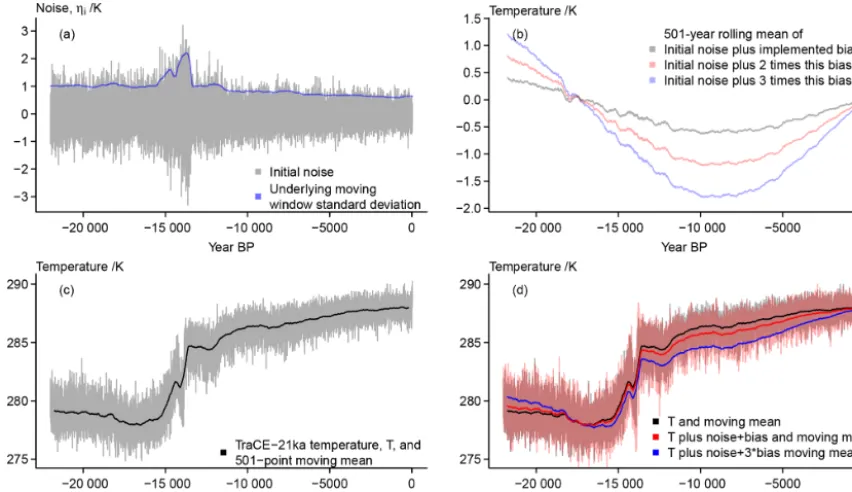
Figure 2a shows an example of the initial noise ηi. The dependence on the background state is clearly visible for the visualized grid point data. There is an increase during the deglaciation and a multi-millennial reduction over the Holocene. Indeed, Rehfeld et al. (2018) diagnose a reduc-tion in temperature variability from the Last Glacial Maxi-mum to the Holocene by studying centennial to millennial timescales.
Panel (b) of Fig. 2 compares three potential amplitudes of the orbitally induced bias. We use the version with the smallest amplitude. Panel (c) of Fig. 2 presents the grid point temperature of the TraCE-21ka simulation and a simple 501-year running mean. The comparison with Fig. 2d highlights that the effect of the bias is rather small given our choice of its amplitude. Nevertheless, comparing the panels also clar-ifies that our implementation of the bias results in a colder annual record over most of the considered time period while the record becomes slightly warmer in the very early portion of the simulated data.
3.2 Assumptions on essential error sources 2: archive
Modifica-O. Bothe et al.: Noise and pseudoproxies 1135
Figure 2.Visualizing considered error sources at the sensor stage:(a)the initial noise and the underlying moving window standard deviations of the input signal,(b)three versions of a potential bias as function of the local insolation,(c)the input data and their 501-point moving mean, (d)the input data and their 501-point moving mean plus noise and bias. The unsmoothed initial temperature is effectively hidden behind the unsmoothed temperature plus bias.
tions include selective destruction of parts of the record by processes acting all the time or by sparse random events or continually acting random processes. Examples are biotur-bation or resuspension. These processes may result in either a correlated noise in time and space or simply white noise. Other de facto white noise errors may result from our finite and random sampling of the archive. However, this may be rather part of the observational noise.
Such modifications of the archive and sampling issues rep-resent an important step in using inverse reconstruction meth-ods because it is a priori not clear how the archive is gen-erated and whether an individual measurement represents mean environmental states or relates to single events. In this context, forward models and pseudoproxy approaches of sed-imentary proxies are a crucial tool in disentangling the con-trolling climatic environmental factors in the generation of sediment cores and their interpretation.
3.2.1 Smoothing and noise
Because we focus on sedimentary proxies, we argue that the archiving process foremost is a filter of variability above a certain frequency level, for example, by diffusive pro-cesses or bioturbation (compare Dolman and Laepple, 2018, and their references). Dependent on the system in question this may only affect the very high frequencies but for other systems it may extend to multi-decadal or even centennial to millennial frequencies. On top of this smoothing of the
archive, there may be additional noise as the smoothing func-tion is unlikely homogeneous. We assume such a filtering to be the fundamental modification of the record in the archive, and, thus, only consider this process in our archive mod-elling.
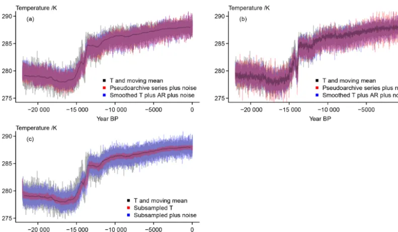
Inspired by the simple proxy forward formulations of Laepple and Huybers (2013, see also Dolman and Laepple, 2018), we produce five different versions of the archived pseudoproxy series. The first and second series are simple running averages of the sensor record to which we add a highly autocorrelated AR process of order one. The two ver-sions differ in the length of the averaging window, the AR coefficients, and the standard deviations of the innovations. Versions three and four similarly differ in the amount of aver-age smoothing, but we use random window lengths for each date. The rationale for the two different smoothing lengths is to represent both strongly and only slightly smoothed prox-ies.
The fifth version aims to mimic the behaviour of proxies when researchers use only a small part of an available proxy, e.g. pick only a certain number of samples. An example is the simple forward formulation for Mg/Ca proxies by Laepple and Huybers (2013, see also Dolman and Laepple, 2018).
pro-vided data use an approach where the random smoothing lengths follow an autoregressive process around a climate-dependent reference smoothing length, where, considering Vardaro et al. (2009), warmer climates result in shorter smoothing intervals. The smoothed archive records are then either
PT(t)=g1(T(t)+ηi(t)+bias(t), t), (6)
whereg1(t) is the time-dependent filter, or
PT(t)=g2(T(t)+ηi(t)+bias(t))+AR, (7)
whereg2is the constant smoothing and we add an AR pro-cess to account for the inhomogeneities in the smoothing.
The fifth version of the pseudoproxy subsamples over the random filter interval and adds a noise term to mimic a sea-sonal uncertainty. That is, we samplenyears within the fil-ter infil-terval, and take the mean over the temperature and the noise for these years. We add another noise term to repre-sent the intra-annual seasonal uncertainty.PT in this case be-comes
PT =h(T(t), t)+h(ηi(t), t)+ηs, (8)
where h(t) represents the subsampling and ηs the intra-annual noise. We do not include the bias term for the sub-sampled proxies. We apply the bias only for the mean annual temperature; i.e. individual seasons show different biases. While we could account for this by sampling the biases over the different seasons or even months in producingh(t) orηs,
we prefer to keep our model simpler. Excluding the bias term may be interpreted as the seasonal subsampling cancelling out the bias. In reality any cancellation would not result in a convergence on the simulated climate state but more likely on a recorded value between the biased and the “true” climate. The coded version of the subsampling still includes the bias term as a comment.
3.2.2 Results
The biased moving average already shows the differences between the target temperature and the pseudoproxy record (compare Fig. 2). The pseudoarchive series in Fig. 3a shows this more clearly. Here we use a randomized smoothing inter-val. Differences are less visible for shorter random smooth-ing intervals (compare Fig. 3b). Further panels of Fig. 3 add the constant smoothing archive approximations which we modify by an additional highly correlated AR process (Fig. 3c and d). This procedure randomly amplifies, damp-ens, or inverts certain biases in the presented case. That is, while the simple random smoothing may emphasize the bias, the AR procedure overlies this bias with additional varia-tions.
The panels highlight an apparent offset between the ran-domly smoothed archive series, the constantly smoothed
archive series, and the smoothed input data. The smoothed version of the input data as well as the constant filtering use a centred approach, that is they are symmetric about their date. The time-varying smoothing tries more realistically to imitate a bioturbation approach (compare Dolman and Laep-ple, 2018, and their references) and thus provides a shift in the series.
Figure 3a also shows the seasonally subsampled pseu-doarchive proxy. The data ignore the bias term and the result-ing series is by construction symmetric around the original data, our target. Nevertheless, there are pronounced devia-tions from the original data. Considering only the deviadevia-tions from the target temperature moving mean highlights that this approach is notably more noisy than the filtered data but pre-serves pronounced longer-term excursions of the input data (not shown).
3.3 Assumptions on essential error sources 3: measurements
The archiving represents also a transformation from time units to archive distance units, to depths, rings, distances. The proxy becomes a tuple of date and data. Now the dates are un-certain as each data point includes information from different original dates due to the smoothing function. The sampling may lead to additional uncertainties due to disturbances of the archive, and the dating of our samples is a profoundly uncertain process.
3.3.1 Measurement error
O. Bothe et al.: Noise and pseudoproxies 1137
Figure 3.Visualizing considered error sources at the archive stage:(a)501-year moving mean of the input data, the pseudoarchive series with longer average smoothing lengths, and the subsampled record;(b)501-year moving mean of the input data, the pseudoarchive series with shorter average smoothing lengths,(c)501-year moving mean of the input data, the pseudoarchive series with longer average smoothing lengths, and the version with constant smoothing and added AR(1) process;(d)501-year moving mean of the input data, the pseudoarchive series with shorter average smoothing lengths, and the version with shorter constant smoothing and added AR(1) process.
We apply the measurement error term at the end. However, we introduce this term before dealing with the dating uncer-tainty since we provide proxies without dating unceruncer-tainty. The measured proxy series becomes
MT =PT+ηM. (9)
In reality, we do not have a continuously sampled series, but obtain only samples at certain intervals. Assuming N sam-ples the sampled pseudoproxy becomes
PPT =PT(t= {t1, . . ., tN}). (10)
The sampling of the archive likely produces errors in the samples. We assume these are included in the measurement uncertainty. We provide at each grid point sampled series of the pseudoproxies detailed above. We do not distinguish be-tween different sampling techniques. We simply sample the records at certain dates and add the described noise term.
3.3.2 Dating uncertainty
Dating uncertainty represents a big part of our overall un-certainty for many proxies, especially for sedimentary proxy records. In our framework, the smoothing function already redistributes information from one date across the archive. Usually one considers this temporal uncertainty separately from the proxy record error. For assessing reconstruction
methods and simulations, it would be beneficial to be able to include dating uncertainty within the proxy error. That is, if we consider proxies as tuples of data and date, we have to transform the uncertainty of the date into an error term for the data. In the following we distinguish between the dating uncertainty, that is the uncertainty that a sample is from a certain date, and the dating error, by which we mean the po-tential error in our (pseudo)proxy due to the uncertain dating. There are a number of approaches to transfer the dating uncertainty towards the proxy record error (e.g. Breitenbach et al., 2012; Goswami et al., 2014; Boers et al., 2017). En-semble and Bayesian age–depth modelling approaches also allow us to infer an additional error term (e.g. Haslett and Parnell, 2008; Blaauw and Christen, 2011). However in the present application, we want to capture the error in a time series. Thus, we take a very simple approach, which assumes that the error due to dating uncertainties is related to the cli-mate state over the period of the dating uncertainty. Never-theless, since we provide sample dates and random sampling uncertainties, the application of age modelling to the pseudo-proxies is in principle possible (e.g. following the approach of Dee et al., 2015, 2018).
larger portions of the proxy record. The following general approach is common to all variations in our procedure. First, we sample uncertainties in time for each sample date. We take these as dating uncertainty standard deviations. These uncertainties can be sampled fully randomly or dependent on the available smoothing interval data from the archive stage. Then we take the effective dating error at each sample date and depth to be a random sample from a normal distribution. The mean of this distribution is the difference between the sample data and the mean over the data within plus and mi-nus 2 dating uncertainty standard deviations. The standard deviation of the distribution is the standard deviation of the differences between the individual data points within this in-terval and this mean. The effective dating error is then
D=N(PTD, σ
2
D), (11)
where
PTD=PT(tS= {ti−2σdating, . . ., ti, . . ., ti+2σdating})
−PT(t=ti) (12) is the mean over the region of influence and
σD2=E[(PT(tS)−PTD)
2] (13)
is the variance of the distribution.
In the simplest formulation ignoring the dependence be-tween subsequent dates, the sampled pseudoproxies become
PPT(t1, . . ., tN)=g(T(t)+ηi(t)+bias(t), t)
(t1, . . ., tN)+D(t1, . . ., tN). (14) Alternative formulations of the pseudoproxy become
PPT(t1, . . ., tN)=g(T(t)+ηi(t)+bias(t))(t1, . . ., tN)
+AR(t1, . . ., tN)+D(t1, . . ., tN) (15) or
PPT(t1, . . ., tN)=h(T(t), t)(t1, . . ., tN)+h(ηi(t), t)
(t1, . . ., tN)+ηs(t1, . . ., tN)
+D(t1, . . ., tN) . (16) This initial formulation of the effective dating uncertainty er-ror ignores potential correlation between the dating erer-rors. The most simple way to account for this makes subsequent errors dependent:
Di=ρ·(ξDi−1+(PPT i−1−PPT i))+ξDi. (17)
This formulation has only a minor influence on the results. It is included in the code via a binary switch.
A slightly more complex formulation makes the error term at each date dependent on the previous sample’s age uncer-tainties and mean data. Previous refers to archive units in-stead of time units. Then the dating error becomes
Di=ρ·(Di−1+(PPT i−1−PPT i))+ξDi, (18)
whereξDi represents the random innovations for datei. Our
initial choice ofρ=0.9 can give large effective dating uncer-tainty errors. A switch in the code allows the use of this inter-dependent error. Another switch allows the consideration of the dependence between samples as a function of their dates and the dating uncertainty,
ρ(t)=1−(ti−ti−1)/(2·σd(i−1)). (19)
The time-dependent dating uncertainty for each dateσd(t) is
generated randomly (compare aboveσD). We provide data
for the case with a time-dependentρ(t).
Alternative simple formulations may include different noise processes like noise generated from gamma distribu-tions. The available smoothing interval data can inform the sampled dating uncertainty. We could further use this infor-mation to provide a deterministic, not random, error for each sampled date; that is we could take a bias based on all dates influencing the selected date within the dating uncertainty.
In our current setup the age uncertainty does not depend on the measurement noise. The measurement error is added afterwards to the series including the effective dating un-certainty error. This decision is arbitrary. On the one hand a classical dating uncertainty affects the measured value. Then,PPT above should also already include the
measure-ment error. On the other hand, the dating uncertainty affects the archived values independent of the measurement noise. Therefore we keep both independent.
The measured proxy series becomes
MT =PPT +ηM. (20)
The final proxy is in temperature units as are the initial input data. We ignore a separate term for potentially non-linear and climate-state-dependent errors in our calibration relationship and assume the measurement noise term accounts for this as well. A separate term could again be a state-dependent Gaus-sian noise. It could also be a noise from a skewed distribu-tion whose mode depends on the background climate. Con-versely, a state-dependent bias term could simulate a mis-specified calibration relation while a time-dependent bias term could simulate a degenerative effect over time within the archived series. None of these are included in the current version.
3.3.3 Results
O. Bothe et al.: Noise and pseudoproxies 1139
Figure 4.Visualizing considered error sources at the measurement stage for the full series:(a)501-year moving mean of the input data, the pseudoarchive series with longer average smoothing lengths, and the constant smoothing plus AR series with added measurement noise; (b)501-year moving mean of the input data, the pseudoarchive series with shorter average smoothing lengths, and the constant smoothing plus AR series with added measurement noise;(c)501-year moving mean of the input data, the subsampled record, and the subsampled record with added measurement noise.
respectively. Figure 4c plots the seasonally subsampled pseu-doproxy. The final versions of the pseudoproxies generally preserve previously included biases.
Figure 5 presents a number of series sampled atN =200 dates. All panels include the original temperature data sam-pled at these 200 dates. The figure emphasizes how the initial temperature variability at the chosen grid point is generally slightly larger than any of our uncertainty estimates. Our ef-fective dating uncertainty error seldom results in large de-viations from the archived record. The subsequently applied measurement error also only seldom leads to large offsets compared to either the original data or the effectively date-uncertain record. Thus, for our chosen parameter settings and the shown grid point, the pseudoproxies fall within the range of the initial estimates. In turn, if we assume we have reliable calibration relationships, our calibrated proxy series should also be reliable estimates of the past states.
Nevertheless, the biased estimates occasionally are only bad matches for the original data. This is also the case for the subsampled data where we did not include the bias. Compar-ing the sampled pseudoproxy series to the smoothed original temperature data (compare Fig. 5a) highlights that estimates for past climates may well fall within the range of the origi-nal interannual temperature variability but may nevertheless strongly misrepresent the mean climate represented by the sample.
Considering the effective dating uncertainty error, the dis-crepancies between input data and pseudoproxy are rather
small for uncorrelated or weakly correlated age uncertain-ties. However, in the case of strong dependencies between subsequent data, pronounced biases and mismatches may oc-cur (not shown). The assumed co-relation between two dates has a strong influence on the size of these mismatches. We show the case for a time-dependent co-relation between sub-sequent dates, which gives intermediately sized mismatches.
3.4 General results
Figures 2 to 4 present the different versions of the pseudo-proxies for the chosen location. Under our assumptions, the influence of the orbital bias term is notable. The approaches using time-dependent smoothing or simple smoothing plus an AR process may nearly or fully cancel the bias. This ef-fect is less prominent for the time-dependent filter. Generally, both approaches seem to have similar effects.
Figure 5.Visualizing the sampled records:(a)input data and their 501-year moving mean, the pseudoarchive series with longer average smoothing lengths plus the effective dating error and plus the effective dating error and measurement noise;(b)input data and their 501-year moving mean, the constantly smoothed record with longer smoothing length plus AR series with added effective dating error and with added effective dating error and measurement noise;(c)input data and their 501-year moving mean, the pseudoarchive series with shorter average smoothing lengths plus the effective dating error and plus the effective dating error and measurement noise;(d)input data and their 501-year moving mean, the constantly smoothed record with shorter smoothing length plus AR series with added effective dating error and with added effective dating error and measurement noise;(e)input data and their 501-year moving mean, the subsampled record with added effective dating error and with added effective dating error and measurement noise.
interannual data. The document assets provide equivalent vi-sualizations for another grid point. These generally confirm the above descriptions.
3.4.1 Spectral power
Figure 6 adds a comparison of power spectral densities com-puted from a wavelet-based approach similar to the weighted wavelet Z-transform of Foster (1996). The approach is de-scribed by Mathias et al. (2004) and McKay and colleagues provide a compiled version at https://github.com/nickmckay/ nuspectral (last access: 11 March 2019) (McKay et al., 2019). Due to the length of computation, we do not show the density for the full 22 040-year input data but only for a record
sam-pled every 10 years. Results may be specific for the chosen grid point.
The figure shows estimates for the full records and for the data of the last 12 000 years of the records. Spectral densities for the regularly sampled original temperature data in Fig. 6a highlight that the differentiation between full and late records results in prominent differences for multi-centennial to mil-lennial periods. Conversely, differences are smaller for the irregularly sampled input temperature data but still notable for millennial periods. However, there is an offset between the irregularly sampled data and the regularly sampled input data.
O. Bothe et al.: Noise and pseudoproxies 1141
Figure 6.Wavelet-based power spectral densities (Mathias et al., 2004; McKay et al., 2019). Densities are weighted following Mathias et al. (2004) to smooth the records for ease of comparison. Lines are for records split up by the first 10 k years of the records and the last 12 k years of the records. Input data refer to the input data at 10-year intervals. All panels include the late input data from the TraCE-21ka simulation as black lines; red lines are in all panels for a full period record; blue lines are in all panels for the last 12 k years of the version of a pseudoproxy. In addition to the input data from the TraCE-21ka simulation the panels show:(a)the sampled TraCE-21ka simulation input data,(b)the sampled pseudoarchive series with long average smoothing plus the effective dating error and the measurement noise (long random smoothingMT),(c)the constantly smoothed record with a longer smoothing plus an AR(1) process and including the effective dating error and the measurement noise (long constant smoothingMT),(d)the sampled pseudoarchive series with short average smoothing plus the effective dating error and the measurement noise (short random smoothingMT),(e)the constantly smoothed record with a shorter smoothing plus an AR(1) process and including the effective dating error and the measurement noise (short constant smoothingMT),(f)the subsampled data plus the effective dating error and the measurement noise (MT from subsampling).
smaller than in Fig. 6a. Differences between sampled late and full records are often largest at intermediate millennial peri-ods. Deviations are largest for the subsampled pseudoproxy approach at long periods (Fig. 6f) but they also become no-table for the constant smoothing approaches at shorter peri-ods in the centennial band (Fig. 6c, e). This is mainly due to the characteristics of the full period spectra for the constant smoothing, which show an increase in power spectral density for shorter and longer periods. That is, the constant smooth-ing full period spectra are similar to grey noise spectra. De-spite these differences and the apparent offset to the input data spectra, the irregularly sampled spectra for all cases are rather similar.
3.4.2 Global data
The supplementary assets for this paper include plots of se-lected series from our analyses at all grid points starting from the south towards the north (supplementary document 1 Fig. 1 at https://doi.org/10.17605/OSF.IO/ZBEHX/). These
series are the input data at the grid point, the smoothed-plus-AR-process series at the grid point, and its subsampled ver-sion including all uncertainties.
pseudo-Figure 7.Point by point correlation maps between input data and the smoothed record plus AR(1) process plus effective dating error and measurement noise for the sample dates within the first(a), second(b), and third(c)subsequent 5000-year windows of the record and the samples within the remaining years (d).
O. Bothe et al.: Noise and pseudoproxies 1143
proxy on they axis against the original data on thex axis for a small selection of grid points, highlighting the common lack of a clear relation besides the deglaciation.
Figure 7 provides correlation coefficients between the sampled interannual grid point data and the pseudoproxies including all uncertainties for the strong smoothing plus AR. The four panels show correlations for those samples within the first, second, and third 5000-year chunks of the original data, and those samples in the remaining years. We choose to present the data this way to avoid detrending the data over the deglaciation interval. Relations between original data and pseudoproxies are generally weakest in the tropical belt. In the period until present, correlations are overall weak. High-latitude correlations are most notable during the deglacia-tion and slightly less notable during the first millennia of the Holocene. In these periods, correlations appear to be largest in areas with glacial remnants.
Figure 8 adds for the first, the last, and the full period the relative standard deviationσT21k/σP in the left column and the bias T¯T21k− ¯TP in the right column. T21k refers to the simulation,P to the pseudoproxies. For the standard devia-tion ratios, we use 501-year moving averages of the TraCE-21ka data. Variability is generally larger in the pseudoprox-ies except for the North Atlantic and the northern high lati-tudes in the early period, and it is larger in the pseudoproxies more or less everywhere in the late period. Over the full pe-riod, variability is notably larger mainly in the tropics and the Southern Hemisphere; it is about equal over Antarctica and wide regions of the Northern Hemisphere. The variability is clearly larger in the input data only over a small region in the northern Pacific.
The overall largest bias occurs off the coast of southeastern Greenland in the early period in Fig. 8. Otherwise there is a spatial separation between the mid-latitudes to high latitudes and the tropics and subtropics for both periods. The bias is more prominent in the higher latitudes where it is predom-inantly positive in the early period but predompredom-inantly nega-tive in the late period. Obviously, the general latitudinal bias pattern is by construction because we construct the bias as a function of latitudinal insolation.
3.5 On generalizations of the errors
While we already chose comparatively simple procedures for our approach to obtain pseudoproxies from a model simula-tion, it is likely possible to simplify these to a higher degree. Such a general expression for the error in proxies over multi-millennial timescales may be more usable in a number of ad hoc model evaluations and model–data comparisons. Most importantly, such a generalized approach also allows us to quickly produce ensembles of pseudoproxies.
Following our previous assumptions, the easiest way to obtain such a generalized error model would be to assume a simple, potentially correlated noise model for the sensitivity of the sensor to the environment. Here, we use an AR
pro-cess of order one with AR coefficientφ=0.7. Either here or later one scales the series or adds a bias term to account for changing seasonality over multi-millennial timescales. The sum of the input data and this error are then subject to a sim-ple moving averaging function. On top of this another simsim-ple correlated noise process mimics that the redistribution in the archive is not constant in time. Another random component accounts for the measurement error. Thus, simple correlated noise may be enough to catch the essence of the error. In short, the generalized pseudoproxy becomes
MT(t1, . . ., tN)=g(T(t)+ηit+bias(t))
+D(t1, . . ., tN)+ηM , (21)
wheregis the smoothing,ηi is the initial noise, bias is the bias term,Dis the effective dating error, andηMis the mea-surement error. This is conceptually identical to the smooth-ing plus AR approach presented above. Its derivation is less grounded in real proxies. The provided data differ only in the amount of autocorrelation in the noise terms.
Figure 9 summarizes results for the generalized approach. It clarifies that while an error may mask certain features of the past climate evolution, this simple generalized pseudo-proxy generation is unlikely to distort the pseudo-proxy completely if we take the assumptions made above to be approximately appropriate. Interestingly, the generalization appears to mod-ify the input signal slightly less than the more complex ap-proach. However, as we display slightly different data com-parisons here, it is more appropriate to note that the dating uncertainty has only a minor effect compared to the initial bias and AR process modifications and compared to the sub-sequent addition of the measurement noise.
While researchers may validly wish for such simplified recipes for producing pseudoproxies, using a full or at least more complex process-based approach is advisable, if it is necessary to account for effects of biology, environmental long-term changes, and other weakly constrained uncertain-ties. More complex approaches further allow to better mimic non-linearities between the climate and sensor and thus a truly non-linear pseudoproxy.
3.5.1 Ensemble of pseudoproxies
Figure 9.Visualizing the simplified essence of the surrogate proxy calculations:(a)input data and 501-point moving mean;(b)input data plus initial noise and bias term;(c)moving mean of input data plus noise plus bias and the same record plus an AR(1) process; (d)smoothed temperature plus noise plus bias plus AR process sam-pled at 200 dates, this record plus the effective dating error, and this record plus the effective dating error and measurement noise; (e)smoothed temperature plus noise plus bias plus AR process sam-pled at 100 dates, this record plus the effective dating error, and this record plus the effective dating error and measurement noise.
Modifications to the code are as follows. First, we use a number of parameter values sampled from either uniform distributions around the otherwise fixed value or a list of val-ues. Second, we consider random orientations for bias and moving standard deviations; that is we take S asSu where we sample u from U= {−1,1}. We provide the script for the ensemble production as supplementary example code at https://doi.org/10.17605/OSF.IO/ZBEHX. As mentioned
Figure 10.Map of the locations for the ensemble of surrogate prox-ies.
above, these changes relax our assumptions on the effect of changes in the background climate.
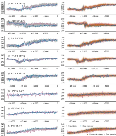
For Fig. 11 we select eight locations to represent the lo-cally diverse representations of the climate in the TraCE-21ka simulation and how the ensemble of pseudoproxies modifies this. The figure provides an impression of the range of the local ensembles and of two random ensemble members around the original temperature series. The diversity of the local climates in TraCE-21ka carries over to individual pseu-doproxies and their ensembles. In addition to this, Fig. 11 mainly reflects the results of previous sections regarding how constrained our pseudoproxies are. However, we commonly see pseudoproxies and ensembles exceeding the variability of the original temperature data, not least because of our modi-fications to the selection of parameters and the orientation of the bias about its mean.
3.6 Provided data
Tables 1 to 4 detail the provided data files. All files are in netcdf format. These are generally gridded files on the orig-inal TraCE-21ka grid. Only the ensembles of pseudoproxies are provided at their respective individual grid points. The data repository at https://doi.org/10.17605/OSF.IO/ZBEHX provides instructions on how to access the file structures.
4 Code and data availability
O. Bothe et al.: Noise and pseudoproxies 1145
Figure 11.Visualizing the surrogate proxy ensemble at selected locations (longitude and latitude in top left corners of the left column panels). The left column shows the input data plotted as grey lines, and two random members of the ensemble as blue and purple lines. The right column plots the range of the ensemble transparently shaded brown, and blue and purple lines are the same two random members. The
xaxes are years BP. The panel on the bottom right shows the figure legend.
5 Conclusions and outlook
This publication presents a flexible yet simple approach for describing the error originating from climatic and non-climatic sources in proxy records over multi-millennial timescales including the last deglaciation. The assumptions are relatively simple but they are based on similar assump-tions for process-based proxy system forward models.
The approach can be easily extended to compute ensem-bles of proxies for single locations. We chose to give one set of pseudoproxies for each grid point of the TraCE-21ka
Table 1.List of files provided, the variables included, their description, the category (full surrogate proxy field, essence field, or ensemble), and size of the ensemble. All files have the same stem Bothe_Trace21k_Pseudo_Proxies_ and the ending _annual.nc.
Filename Variable name Variable description Category Grid Ensemble
size size
Bothe_Trace21k_Pseudo_Proxies_
noise.save noise.save initial environmental noise field 96×48 1
bias.noise.data.save bias.noise.data.save data+noise+bias field 96×48 1
smooth.save smooth.save smoothed data+noise+bias field 96×48 1
meas.noise.smooth.save meas.noise.smooth.save smoothed data+noise+bias plus measure-ment noise
field 96×48 1
ar.smooth.save ar.smooth.save constantly smoothed plus AR process field 96×48 1 meas.noise.ar.smooth.save meas.noise.ar.smooth.save constantly smoothed plus AR plus
measure-ment noise
field 96×48 1
short.smooth.save short.smooth.save smoothed date + noise+ bias for shorter smoothing
field 96×48 1
meas.noise.short.smooth.save meas.noise.short.smooth.save smoothed data+noise+bias plus measure-ment noise for shorter smoothing
field 96×48 1
short.ar.smooth.save short.ar.smooth.save constantly smoothed plus AR process for shorter smoothing
field 96×48 1
meas.noise.short.ar.smooth.save meas.noise.short.ar.smooth.save constantly smoothed plus AR plus measure-ment noise for shorter smoothing
field 96×48 1
subsampled.save subsampled.save seasonally subsampled data+initial noise field 96×48 1 meas.noise.subsampled.save meas.noise.subsampled.save seasonally subsampled+noise plus
measure-ment noise
field 96×48 1
Table 2.Continued list of files provided, the variables included, their description, the category (full surrogate proxy field, essence field, or ensemble), and size of the ensemble. All files have the same stem Bothe_Trace21k_Pseudo_Proxies_ and the ending _annual.nc.
Filename Variable name Variable description Category Grid size Ensemble size
sampled samp.subsampled.save, samp.meas.noise.smooth.save,
samp.input.save, samp.input.save.short, samp.input.save.ar,
samp.input.save.ar.short, samp.noise.save, samp.noise.save.short, samp.noise.save.ar, samp.noise.save.ar.short,
samp.bias.noise.data.save, samp.bias.noise.data.save.short, samp.bias.noise.data.save.ar, samp.bias.noise.data.save.ar.short, samp.ar.smooth.save, samp.smooth.save, samp.short.smooth.save,
samp.short.ar.smooth.save, samp.meas.noise.short.smooth.save, samp.dates.save, samp.dates.save.short, samp.dates.save.ar,samp.dates.save.ar.short, samp.meas.noise.ar.smooth.save,
samp.meas.noise.short.ar.smooth.save, samp.meas.noise.subsampled.save
sampled versions of the various variables and the dates of the samples
field 96×48 1
We choose only one possible set of parameters in our pseu-doproxy model, but we sample around this set for the ensem-ble of pseudoproxies. We choose these specific parameters to provide some disturbance to the data but not to get anywhere too far away from the original state. For example, it is quite likely that we have to face larger biases in reality than rep-resented by our choice. Users should make their own choice
of parameters according to their assumptions on the various noise contributions.
con-O. Bothe et al.: Noise and pseudoproxies 1147
Table 3.Continued list of files provided, the variables included, their description, the category (full surrogate proxy field, essence field, or ensemble), and size of the ensemble. All files have the same stem Bothe_Trace21k_Pseudo_Proxies_ and the ending _annual.nc.
Filename Variable name Variable description Category Grid size Ensemble size
dating-error samp.dates.save, samp.dates.save.short, samp.dates.save.ar,samp.dates.save.ar.short,
unc.date.samp, unc.date.samp.short, unc.date.samp.ar, unc.date.samp.ar.short, unc.date.subsampled.save, unc.date.meas.noise.smooth.save, unc.date.noise.save, unc.date.bias.noise.data.save, unc.date.ar.smooth.save, unc.date.smooth.save, unc.date.short.smooth.save, unc.date.short.ar.smooth.save,
unc.date.meas.noise.short.smooth.save, unc.date.meas.noise.ar.smooth.save, unc.date.meas.noise.short.ar.smooth.save, unc.samp.meas.noise.subsampled.save
date uncertain versions of the various variables and the dating uncertainties
field 96×48 1
Table 4.Continued list of files provided, the variables included, their description, the category (full surrogate proxy field, essence field, or ensemble), and size of the ensemble. All files have the same stem Bothe_Trace21k_Pseudo_Proxies_ and the ending _annual.nc.
Filename Variable name Variable description Category Grid Ensemble
size size
Essence_gen.noise.env gen.noise.env generalized environmental noise term
essence 96×48 1
Essence_noise.gen.dat noise.gen.dat input data+generalized environmental noise
essence 96×48 1
Essence_bias.noise.gen.dat bias.noise.gen.dat input data+generalized noise +bias term
essence 96×48 1
Essence_smooth.bias.noise.gen.dat smooth.bias.noise.gen.dat smoothed input+noise+bias essence 96×48 1 Essence_ar.smooth.bias.noise.gen.dat ar.smooth.bias.noise.gen.dat smoothed input+noise+bias
plus AR process
essence 96×48 1
Essence_uncertain-sampled samp.ar.smooth.bias.noise.gen.dat, unc.samp.ar.smooth.bias.noise.gen.dat, meas.unc.samp.ar.smooth.bias.noise.gen.dat, unc.date.samp.gen, samp.dates.save.gen
date uncertain versions of gen-eralized data, gengen-eralized dat-ing uncertainty, sample dates
essence 96×48 1
essence_ensemble Pseudoproxy, Dates, DateUncertainty surrogate proxy data, dating, uncertainty of dating
ensemble 144 500
Lat, Lon latitude, longitude ensemble 144 1
sidering an effective dating uncertainty error for the pseudo-proxy data. Similarly, we do not consider spatial correlations in the noise. Such correlations between locations are prob-ably relevant for some noise terms while they are probprob-ably less important for others.
We focused on the time series approach and did not choose a probabilistic approach like, for example, Breitenbach et al. (2012) or Goswami et al. (2014). Neither does our approach as of now explicitly link to probabilistic age modelling ap-proaches as described by Haslett and Parnell (2008), Blaauw and Christen (2011), or Trachsel and Telford (2017).
There are a variety of other potential approaches to ob-taining simple pseudoproxies from the model data. One such example would be to consider an envelope around the model state, to randomly select a set of dates from the original data, fit a smooth through this set, and then sample again around this uncertain smoothing. Similarly, Gaussian process mod-els or generalized additive modmod-els may be valuable means in producing pseudoproxies for paleo-climate studies over
timescales longer than the common era of the last 2000 years. For example, Simpson (2018) shows the benefits of general-ized additive models for studies on paleo-environmental time series.
Appendix A: Tables of parameters
Tables A1 to A4 summarize the considered parameters and noise models. They also clarify whether the parameter set-tings are used for a global field of surrogate proxies, a more generalized approach, an ensemble calculation, or all.
Table A1.List of parameters used.
Description Parameter Value Category
Season limits for insolation bias mon1.for.insol, mon2.for.insol 1, 12 all
Number of samples along the full record n.samples 200 all
Scaling of initial noise amplitude amp.noise.env 0.5 field, essence
Switch for proportionality of initial noise switch.orient.runsd.noise.env 0 all
Model for the initial noise model.noise.1 c(0.3) field, essence
Standard deviation of innovations for initial noise sd.noise.1 not used field, essence Length of window influencing initial noise length.window.runsd 1000 field, essence
Switch for orientation of bias switch.orient.bias.seas 0 all
Scaling of bias term amp.bias.seas 4 field, essence
Table A2.Continuation of list of parameters used.
Description Parameter Value Category
Switch for smoothing variant switch.smoothing 3 field
Secondary switch for smoothing, see code switch.sm.2 1 field
Scaling for climate dependence of smoothing scale.sm 1/10 field
Mean smoothing length for longer random smoothing rand.mean.length.smooth 350 field Standard deviation for longer random smoothing rand.sd.length.smooth 75 field
Model for longer alternative smoothing model.smooth.1 c(0.99) field
Model for longer alternative climate dependent smoothing model.clim.smooth.1 c(0.9) field Basis long smoothing length for alternative approach rand.length.smooth.mean.1 500 field Standard deviation for longer alternative smoothing approaches sd.model.smooth.1 10 field
Fixed longer smoothing length fix.length.smooth 501 field
Minimum allowed longer random smoothing length min.rand.length.smooth 40 field
AR coefficient for added AR(1) process coeff.ar.smooth 0.999 field
Standard deviation for the innovations sd.ar.smooth 0.01 field
Mean smoothing length for shorter smoothing rand.mean.length.smooth.2 31 field Standard deviation for shorter random smoothing rand.sd.length.smooth.2 5 field
Model for shorter alternative smoothing model.smooth.2 c(0.7) field
Model for shorter alternative climate dependent smoothing model.clim.smooth.2 c(0.9) field Basis short smoothing length for alternative approach rand.length.smooth.mean.2 31 field Standard deviation for shorter alternative smoothing approaches sd.model.smooth.2 4 field
Fixed shorter smoothing length fix.length.smooth.2 31 field
Minimum allowed shorter random smoothing length min.rand.length.smooth.2 5 field
AR coefficient for added AR(1) process coeff.ar.smooth.2 0.9 field
O. Bothe et al.: Noise and pseudoproxies 1149
Table A3.Continuation of list of parameters used.
Description Parameter Value Category
Number of picked samples for subsampling n.samp.pick 30 field
Standard deviation of innovations for subsampling noise sd.noise.pick 0.5 field
Model of subsampling noise model.noise.pick c() field
1.96 sigma of measurement-noise lim.noise.meas 1.5 field, essence
Noise model for measurement noise model.noise.meas c() field, essence
Noise model for measurement noise for subsampled record model.seas.pick.noise.meas c() field 1.96 sigma for measurement noise for subsampled record lim.seas.pick.noise.meas 1.5 field
Switch for correlated effective dating error switch.cor.date.unc 1 all
Switch for weakly correlated only switch.weak.cor.date.unc 1 all
Switch for time dependent correlated switch.delta.cor.date.unc 1 all
Fixed correlated dating error coefficient cor.date.unc 0.9 all
Mean of distribution of dating uncertainty mean.date.unc 350 all
Standard deviation of distribution of dating uncertainty sd.date.unc 100 all Switch for length of influence on dating uncertainty switch.cor.length 1 all
Switch for date sampling switch.sampling 1 all
Switch for dating uncertainty sampling switch.sampling.unc 1 all
Model for initial noise for generalized case model.gen.noise c(0.7) essence
Model for initial noise for generalized case coeff.gen.ar.smooth 0.999 essence, ensemble Standard deviation for AR process innovations, generalized case sd.gen.ar.smooth 0.01 essence, ensemble
Smoothing length generalized case length.filter.uniform 501 essence
Table A4.Continuation of list of parameters used.
Description Parameter Value Category
Ensemble size size.ensemble 500 ensemble
Amplitude of scaling of initial noise amp.noise.env U(0.4,1.5) ensemble
Scaling of bias amp.bias.seas U(3,10) ensemble
Standard deviation of measurement noise lim.noise.meas U(0.75,3)/1.959964 ensemble AR coefficient of measurement noise model rand.model.coeff U(0.3,0.8) ensemble AR coefficient of initial noise model rand.model.coeff.gen U(0.6,0.8) ensemble Window of influence of background climate – not used rand.width.background.sd U(500,2000) ensemble
Window of influence of background climate rand.width.background.sd 1000 ensemble
Width of window of filter influence length.filter.uniform is random sample from ensemble