Prior Specification in Bayesian Model Averaging: An application to Economic Growth

(1)

PRIOR SPECIFICATION IN BAYESIAN MODEL AVERAGING:

AN APPLICATION TO ECONOMIC GROWTH

Tayo P. Ogundunmade, Adedayo A. Adepoju

Department of Statistics, University of Ibadan, Oyo State, Nigeria

Corresponding Author: Tayo P. Ogundunmade, [email protected]

ABSTRACT:Some recent cross-country cross-sectional analyses have employed Bayesian Model Averaging to tackle the

issue of model uncertainty. Bayesian model averaging has become an important tool in empirical settings with large numbers of potential regressors and relatively limited number of observations. We examine the effect of a variety of prior assumptions on the inference, posterior inclusion probabilities of regressors and on predictive performance. Bayesian model averaging (BMA) has become a widely accepted way of accounting for model uncertainty in regression models. However, to implement BMA, a prior is usually specified in two parts: prior for the regression parameters and prior over the model space. Hence, the choice of prior specification becomes paramount in Bayesian inference, unfortunately, in practice, most Bayesian analyses are performed with the so-called non-informative priors (i.e. priors constructed by some formal rule). The arbitrariness in the choice of prior or choosing inappropriate priors often lead to badly behaved posteriors. It is therefore imperative to study the effect of choice of priors in Bayesian model averaging. Six candidate parameter priors namely, Unit information prior (UIP), Risk inflation criterion (RIC), Bayesian Risk Inflation criterion (BRIC), Hannan-Quinn criterion (HQ), Empirical Bayes (EBL) and hyper-g and three model priors: uniform, beta-binomial and binomial were examined in this study. The performances of the resulting eighteen cases were judged using posterior inference, posterior inclusion probabilities of regressors and predictive performance. Analyses were carried out using datasets with 9-potential drivers of growth for 126 countries from 2010 to 2014. Finally, our analysis shows that the EBL parameter prior with random model prior robustly identifies far more growth determinants than other priors.

KEYWORDS: Prior specification, Bayesian Model Averaging, Economic growth, Predictive performance.

1.0 INTRODUCTION

Variable selection process has received considerable attention in the econometrics and statistics literature over the years. The special issues of the Journal of Econometrics (Vol. 16, No. 1, 1981) and Statistica Sinica (Vol. 7, No. 2, 1997) were devoted to the subject of model selection process in view of its relevance. In modelling, functional forms, whether linear or non-linear; error structures, whether addictive or multiplicative; variables inclusion, whether redundant or relevant; and model choice are uncertain. When a single model is selected by considering its highest posterior probability value and later use to make inference, it ignores and underestimates the uncertainties involved in the models. The overall uncertainty about quantities of interest usually lead to unreliable standard error and confidence interval of such model.

A Bayesian tool for dealing with such uncertainties inherent in the model selection process is known as Bayesian Model Averaging (BMA). BMA is used in empirical settings with large amount of possible regressors and relatively limited number of observations to account for uncertainties. It is a weighted averaging method based on posterior distribution which the literature has shown that it provides an improved out of sample predictive performance. Bayesian Model Averaging has been applied successfully to many econometric model classes especially the normal linear regression model [RMH97; RPV05; FLS01a; FLS01b].

(2)

From the literature, the Zellner g-structure in the parameter prior is expected to be as small as possible such that consistency of the true posterior model probability holds. And improving on work of the Fernandez et al. ([FLS01a]) priors, therefore this study focuses on the g-parameter prior elicitation in the BMA approach to normal linear regression model. This modified prior structure allows the marginal likelihood be computed analytically and does not violate the probability rule (not rely on the sample model y). It is independent of input from the researcher or information in the data but depends only on the sample size. Three different model priors and six parameter priors were elicited for this study.

The rest of the paper is divided into four sections. Section II describes the BMA theoretical approach while section III elicits the determinants of economic growth. Section IV shows the results of the data and the analysis and finally, the discussion of the results and concluding remarks are given in section V.

2.0 BAYESIAN MODEL AVERAGING FRAMEWORK

Consider n independent random samples from a normal linear regression model with constant term, , K potential explanatory variables in a matrix X of dimension n x K and a normal IID error term with variance . If are the explanatory variables included in Model j , j = 1, … , M (M = plausible models) which contains the choice of 0 < < K ( is the number of regressors in model j) and then leads to the linear regression model, ‘y' of the form:

(1) In Bayesian paradigm, we may be interested in a quantity or variable ( ) across the entire model space. Hence, the posterior distribution of the quantity of interest, ( ) given the data is as:

(2)

where D is the sample data. Equation (2) is the mixture of the posterior distributions of that quantity under each of the models with the weighted probability model .

Thus,

(3)

Where, is prior probability that is the true model and the Marginal Likelihood is given by

(4)

where h is the model precision, -Marginal likelihood, likelihood of the data and - the prior distribution for the parameters given the model. BMA gets the Posterior Inclusion Probability (PIP) of an explanatory variable by summing the Posterior Model Probabilities across those models that contain the explanatory variable.

Introducing the g parameter prior to (4) and taking its ratio gives us another very important tool in BMA called the Bayes factor ( ) for comparing two models and and can be computed analytically by ([FLS01a])

if (5)

2.1 Priors in BMA

(3)

of thumb. There are other model priors like binomial, beta-binomial and custom prior inclusion probabilities but for this study the binomial, beta-binomial and the uniform model prior are used and are stated as follow:

(6)

The g-parameter priors considered in this study are Unit Information Prior (UIP), Local empirical Bayes, Hyper-g or _xed (Zellner-Hyper-g) prior, Bayesian Risk Ination criterion (BRIC), Hannan-Quinn criterion (HQ), Empirical Bayes (EBL). The g-prior was first introduced under the BMA in [Zel86]. Zellner assumed that covariance of the prior should be proportional to covariance expression of the posterior gotten from the data with the scalar g (to be elicited by the researcher) to determine the degree of importance attributed to the prior precision. And from the literature, this g prior structure has shown that it leads to simple closed form expressions of posterior statistics.

Following from the rule of Thumb, the prior probability for the intercept is

(7) The prior probability for precision is

P (8) Then, the parameter prior is ([Zel86])

(9)

Where, is the mean deviation of and the g-prior is proportional to the comparable data based quantity; the smaller the g, the fewer the prior parameter variance.

Table 1 shows the g-parameter priors elicited in the literature. These g-priors in the BMA are related to a natural conjugate prior with the scalar g to be elicited by the researcher ([Zel86]). The g-prior with unit information prior (UIP), g = (1/n) and g = (1/ ) explaining that the priors contain information approximately equal to that contained in a single typical observation. Also, their resulting posterior model probabilities are closely approximated by Schwarz (SIC) or Bayesian Information Criterion (BIC). They have the same mean and precision except for UIP with maximum likelihood as its mean. Prior 2, it is called Bayesian Risk Inflation Criterion prior. Prior 3 explains the decrease in the prior information even slower with sample size and there is asymptotic convergence to the Hannan Quinn Criterion with CHQ= 1. But if the g-prior elicitation depends only on the regressors like g = 1/ , it is approximated by Risk Inflation Criterion (RIC), the larger the value of K the higher the prior information. Prior can also rely on information from the data with known, the closer the to 1 the smaller the precision and the higher the prior information. This type of g-class (prior 5 of Table 1) is called Hyper-g prior, the data dependent prior as elicited in the work of Raftery et al. ([RMH97]). Another class of g with a natural conjugate prior structure which is subjectively elicited through predictive implications is prior six specification.

(4)

Table 1: The g-Parameter Prior Structures ([EPR09])

Prior Specification of g-prior Comment Source

1 Unit Information Prior The prior contains information approximately equal to that contained in a single typical observation. The resulting posterior model probabilities are closely approximated by the

Schwarz Criterion, BIC.

[KW95;Raf95]

2 BRIC A mechanism that asymptotically converges to the unit information prior (g =N) or the risk in inflation criterion (g =

). That is, the g prior is set to g = max(N; ).

[FLS01b]

3 HQ The Hannan-Quinn criterion. CHQ = 3 as n becomes large. [HQ79]

4 EBL Prior information decreases even slower with sample size and there is asymptotic convergence to the Hannan-Quinn

criterion with CHQ=1.

[HQ79]

5 RIC Sets g = and conforms to the risk inflation criterion [FG94]

6 Hyper - g This option uses a family of priors on g that provides improved mean square risk over ordinary maximum likelihood

estimates in the normal means problem. An advantage of the hyper g prior is that the posterior distribution of g given a

model is available in closed form.

[Stra71]

3.0 DETERMINING GROWTH DETERMINANTS

Since economic growth is the fundamental driver of living standards, it is of great interest to economists and policymakers alike to identify which of the numerous theories proposed receive support from the data and which determinants have a significant effect on growth.

Attempts to identify robust growth determinants date back to Levine and Renelt ([LR92]), who used extreme bounds analysis. Formal BMA analysis was conducted by Brock and Durlauf ([BD01]), Fernandez et al. ([FLS01a]) and Sala-I-martin et al. ([SDM04]). The dataset used across studies always contains a core of at least 41 candidate regressors, motivated by Sala-I-Martin ([Sal97a]) and Fernandez et al. ([FLS01a]).

In this section a time series cross-sectional (panel) data of 126 countries has been used in the analysis. The annual time period ranges from 2010 to 2014. The variables considered for the countries are the GDP, Government Consumption rate, Inflation rate, Fiscal Policy Rate, Unemployment Rate, Industrial Production, Trade Openness, Exchange Rate and Public Debt.

Data for all these variables, was obtained from World Bank World Development Indicators (WDI). Trade openness data was obtained using the simple measure (exports plus imports divided by GDP). For exports, imports and GDP data, these were obtained also from World Bank WDI. For datasets with small numbers of observations, priors play important role.

4.0 ANALYSIS OF RESULTS

In this section we will present Posterior Inference, Posterior Inclusion Probability (PIP) and the Predictive Inference results for three model priors discussed in the methodology above. We focus, in particular, on the effect of the prior choices on posterior model distributions, the spread of the posterior mass over model space, posterior model probabilities and the inclusion of individual regressors.

4.1 Assessment of Prior Distributions Using Posterior Inference

(5)

Table 2: Posterior Inference using Uniform Model Prior (Mean and Standard Deviation)

VARIABLES PARAMETER PRIORS

UIP RIC BRIC HQ EBL HYPER

FISCAL BALANCE 1054.96 1038.78 1054.96 1050.17 995.17 996.29

(168.19) (167.06) (168.19) (167.83) (164.45) (164.53)

GOVERNMENT CONSUMPTION -1634.04 -1533.83 -1634.04 -1586.27 -1450.64 1456.21

(417.83) (386.94) (417.83) (403.86) (371.42) (373.83)

INDUSTRIAL PRODUCTION -533.77 -623.26 -533.77 -583.41 -621.90 -617.37

(343.94) (285.33) (343.94) (318.01) (257.54) (262.12)

TRADE OPENNESS -1159.97 -1380.19 -1159.97 -1280.33 -1384.02 -1373.64

(795.83) (665.49) (795.83) (740.27) (598.76) (609.71)

POLICY INTEREST -32.64 -75.64 -32.64 -47.88 -111.24 -104.51

(105.29) (149.48) (105.29) (124.69) (166.25) (163.33) INFLATION RATE 17.26 36.58 17.26 24.10 53.02 49.93

(54.44) (73.92) (54.45) (62.83) (81.94) (80.53) PUBLIC DEBT 0.8025 2.0908 0.8025 1.2051 3.18 3.50

(6.49) (10.2306) (6.46) (7.87) (13.42) (12.91) EXCHANGE RATE -0.6794 -0.0176 -0.0068 0.0103 -0.031 -0.0285 (0.0648) (0.1026) (0.0648) (0.0792) (0.13) (0.129)

UNEMPLOYMENT RATE 3.0622 7.5331 3.0622 4.5115 13.04 12.05

(30.40) (47.57) (30.40) (36.88) (62.26) (59.898)

Table 3: Posterior Inference using Fixed Model Prior (Mean and Standard Deviation)

FISCAL BALANCE 1054.96 1038.78 1054.96 1050.17 995.17 996.29

(168.19) (167.06) (168.19) (167.83) (164.45) (164.53)

GOVERNMENT CONSUMPTION -1634.03 -1533.83 -1634.04 -1586.27 -1450.64 -1456.21

(417.83) (386.94) (417.83) (403.86) (371.42) (373.83)

INDUSTRIAL PRODUCTION -533.77 -623.26 -533.77 -583.41 -621.90 -617.37

(343.94) (285.33) (343.94) (318.01) (257.54) (262.12)

TRADE OPENNESS -1159.97 -1380.19 -1159.97 -1280.33 -1384.02 -1373.64

(795.83) (665.49) (795.83) (740.27) (598.76) (609.71)

POLICY INTEREST -32.64 -75.64 -32.64 -47.88 -111.24 -104.51

(105.29) (149.48) (105.29) (124.69) (166.25) (163.33)

INFLATION RATE 17.26 36.58 17.26 24.10 53.02 49.93 (54.44) (73.92) (54.45) (62.83) (81.94) (80.53) PUBLIC DEBT 0.8025 2.0908 0.8025 1.2051 3.18 3.50

(6.49) (10.2306) (6.46) (7.87) (13.42) (12.91) EXCHANGE RATE -0.6794 -0.0176 -0.0068 0.0103 -0.031 -0.0285 (0.0648) (0.1026) (0.0648) (0.0792) (0.13) (0.129)

(30.40) (47.57) (30.40) (36.88) (62.26) (59.898)

Table 4: Posterior Inference using Random Model Prior (Mean and Standard Deviation)

FISCAL BALANCE 1058.18 1039.04 1058.18 1051.89 984.51 986.43

(168.52) (167.12) (168.52) (168.04) (163.94) (164.14)

GOVERNMENT CONSUMPTION -1697.67 -1538.33 -1697.67 -1620.22 -1421.73 -1429.57

(433.59) (386.88) (433.59) (416.77) (364.69) (368.17) INDUSTRIAL PRODUCTION -460.28 -618.27 -460.28 -544.398 -630.17 -625.17 (367.38) (290.14) (367.38) (339.34) (242.69) (248.75)

TRADE OPENNESS -992.85 -1369.16 -992.85 -1190.22 -1404.63 -1392.40

(839.21) (674.78) (839.21) (784.01) (561.42) (575.96)

POLICY INTEREST -29.29 -94.07 -29.29 -49.84 -164.32 -154.22

(100.22) (161.40) (100.22) (126.83) (177.88) (176.87) INFLATION RATE 15.54 45.22 17.26 24.95 78.42 73.64

(51.89) (79.61) (54.45) (63.699) (18.50) (87.54) PUBLIC DEBT 0.7644 32.30 0.7644 1.3956 8.1984 7.46

(6.2923) (12.49) (6.29) (8.42) (18.50) (17.81) EXCHANGE RATE -0.0063 -0.02595 -0.0063 -0.0116 -0.0632 -0.0577 (0.0627) (0.1238) (0.0626) (0.0839) (0.1870) (0.1794)

(6)

4.2 Assessment of Prior Distributions Using Posterior Inclusion Probability (PIP)

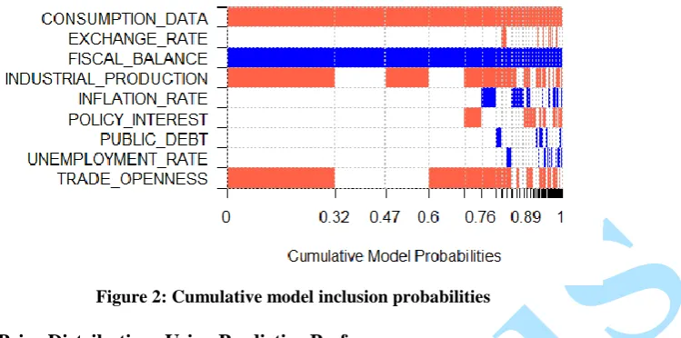
Tables 5, 6 and 7 report the BMA posterior inclusion probabilities for all 6 prior distributions applied to the growth dataset. Table 5 shows the result of the uniform model priors against the 6 parameter priors. Table 6 shows the result for fixed model prior and table 7 for random model prior. Posterior inclusion probabilities and the number of regressors that exhibit evidence of an effect on growth vary substantially across priors. The number of regressors whose inclusion probability exceeds 50% ranges from a low of four regressors (Priors UIP, Hyper and RIC) to a high of 4 regressors (EBL) considering random model prior.

Table 5: Posterior Inclusion Probability (PIP) for Uniform Model Prior

FISCAL BALANCE 0.9999 0.9999 0.9999 0.9999 0.9999 0.9999

GOVERNMENT CONSUMPTION 0.9966 0.9982 0.9966 0.9974 0.9986 0.9985

INDUSTRIAL PRODUCTION 0.7848 0.9164 0.7848 0.8551 0.9496 0.9427

TRADE OPENNESS 0.7578 0.9027 0.7578 0.8342 0.9409 0.9330

POLICY INTEREST 0.1227 0.2838 0.1227 0.1791 0.4368 0.4103

INFLATION RATE 0.1267 0.2762 0.1267 0.1788 0.4430 0.3977

PUBLIC DEBT 0.0479 0.1234 0.0479 0.0717 0.2297 0.2115

EXCHANGE RATE 0.0448 0.1154 0.0448 0.0673 0.2147 0.1977

Table 6: Posterior Inclusion Probability (PIP) for Fixed Model Prior

FISCAL BALANCE 0.9999 0.9999 0.9999 0.9999 0.9999 0.9999

TRADE OPENNESS 0.7578 0.9027 0.7578 0.8342 0.9409 0.9330

POLICY INTEREST 0.1227 0.2838 0.1227 0.1791 0.4368 0.4103

INFLATION RATE 0.1267 0.2762 0.1267 0.1788 0.4230 0.3977 PUBLIC DEBT 0.0479 0.1234 0.0479 0.0717 0.2297 0.2115 EXCHANGE RATE 0.0448 0.1154 0.0448 0.0673 0.2147 0.1977

Table 7: Posterior Inclusion Probability (PIP) for Random Model Prior

FISCAL BALANCE 0.9999 0.9999 0.9999 0.9999 0.9999 0.9999

TRADE OPENNESS 0.6508 0.8950 0.6508 0.7767 0.9637 0.9544

POLICY INTEREST 0.1102 0.3438 0.1101 0.1858 0.6396 0.6112

INFLATION RATE 0.1142 0.2762 0.1267 0.1788 0.4430 0.3977 PUBLIC DEBT 0.0451 0.1837 0.0451 0.0814 0.4740 0.4324 EXCHANGE RATE 0.0420 0.1718 0.0420 0.0760 0.4532 0.4126

(7)

Figure 2: Cumulative model inclusion probabilities

4.3 Assessment of Prior Distributions Using Predictive Performance

We now compare the competing default priors on the basis of predictive performance on hold-out samples, a neutral criterion that allows the comparison of different methods on the same footing. We compare the performance of the full predictive distributions produced by the methods, as well as that of point predictions. We use a proposed method by Theo Eicher ("bma.compare" proposed by Theo Eicher et al.([EPR11]), programmed in R) simultaneously evaluates all 6 different parameter priors and any specific prior expected model size, as well as their predictive performance. We divide the dataset randomly into a training set, , which is used to estimate the BMA predictive distribution, and a hold-out set, , which is used to assess the quality of the resulting predictive distributions. We use three different criteria, or scoring rules: the mean squared error (MSE) of prediction, the log predictive score (LPS; Goo52]), and the continuous ranked probability score (CRPS; [MW76]). All our scoring rules are negatively oriented, that is, lower is better.

The MSE is the most popular measure to assess predictive performance in economics.

It focuses on point estimation, while the LPS and the CRPS assess the entire predictive distribution. The CRPS and the LPS assess both the sharpness of a predictive distribution and its calibration, namely the consistency between the distributional forecasts and the observations. However, the LPS assigns harsh penalties to particularly poor probabilistic forecasts, and can be very sensitive to outliers and extreme events ([WS00; GR07]). This may be a factor when we split our small sample to examine predictive performance. The CRPS is more robust to outliers ([CCB09; GR07]), and hence it is our preferred measure of the performance of the predictive distribution as a whole.

The MSE of prediction is conventionally used to assess the quality of point predictions. The BMA point prediction for an observation in the hold-out dataset , with predictors, , is

The MSE of prediction is then

where is the number of observations in .

The other two scoring rules measure the quality of the predictive distribution as a whole. The BMA predictive distribution is

(8)

Let F be the cumulative distribution function corresponding to the BMA predictive density . Then the CRPS for the single observation is

where if and 0 otherwise. The CRPS for the hold-out dataset as a whole is then

The CRPS measures the area between a step function at the observed value and the predictive cumulative distribution function. Unlike the LPS, it is defined when the prediction is deterministic; in that case it reduces to the mean absolute error ([Her02]). The LPS and the CRPS assess both the sharpness of a predictive distribution and its calibration, namely the consistency between the distributional forecasts and the observations. However, the LPS assigns particularly harsh penalties to poor probabilistic forecasts, and so can be very sensitive to outliers and extreme events ([WS00; GR07]). The CRPS is more robust to outliers ([CCB09; GR07]), and hence it is our preferred measure of the performance of the predictive distribution as a whole. We also report the LPS for comparability with previous work, notably that of Fernandez et al. ([FLS01b; LS07]). We divided the dataset randomly into a training set that contains 80% of the data and thus leaves 20% of the data to be predicted, and we repeated the analysis for 400 different random splits, reporting the average over all splits.

Table 8 shows the predictive performance of the 6 parameter priors in conjunction with uniform, fixed and random model priors as evaluated by the MSE, LPS and CRPS.

The MSE and the CRPS agree that our baseline UIP decisively outperformed all the other priors. The LPS suggests, however, that EBL and BRIC outperform UIP. Since this result runs counter to the results from the two other scoring rules, it seems possible that the difference is due to influential observations in the dataset or outliers in a particular subsample. Several of the regressors have extreme outlying values. When such cases are in the test set, they can have a large effect on the LPS, while the CRPS is more robust to individual cases. Given the known outlier sensitivity of the LPS, we discount the results it gives for this dataset, and conclude that EBL performs best in this case.

Table 8: Parameter priors and predictive performance: performance scores relative to parameter UIP

Prior Uniform model Fixed model Random model

MSE BRIC 0.715 1.000 1.03 HQ 1.08 1.06 0.907 EBL 0.621 0.628 0.969 RIC 0.983 0.767 0.926 HYPER 0.808 0.903 0.786

CRPS BRIC 0.498 0.567 0.525

HQ 0.583 0.556 0.533 EBL 0.454 0.489 0.558 RIC 0.531 0.505 0.543 HYPER 0.539 0.551 0.524

LPS BRIC 160 179 177

HQ 183 183 172

EBL 155 154 176

RIC 170 163 174

HYPER 166 173 164

(9)

derive from the number of iteration counts, while the "exact" PMPs are calculated from comparing the analytical likelihoods of the best models. Both columns sum up to the same number and show that in total, the top 2,000 models of posterior model mass.

Table 9: The MCMC and the Exact Posterior probabilities for the First Best 10 Models

Models PMP (Exact) PMP (MCMC)

021 0.867 0.867

025 0.0255 0.026

031 0.0212 0.02124

0a1 0.0199 0.02

061 0.01879 0.0188

023 0.01766 0.0177

029 0.0177 0.0176

035 0.00097 0.00097

0a5 0.00094 0.00094

065 0.00092 0.00092

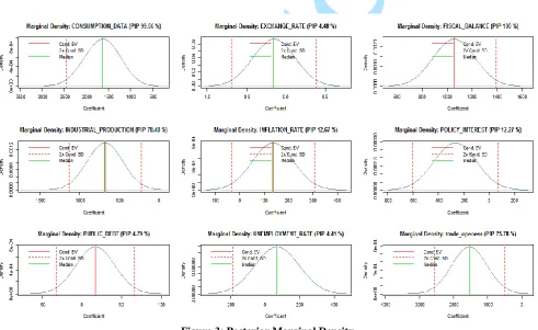
Figure 3 shows the computed marginal posterior densities are a Bayesian model averaging mixture of the marginal posterior densities of the individual models. The accuracy of the result therefore depends on the number of "best" models. Note that the marginal posterior density can be interpreted as "conditional on inclusion": If the posterior inclusion probability of a variable is smaller than one, then some of its posterior density is Dirac at zero. Therefore the integral of the returned density vector adds up to the posterior inclusion probability, i.e., the probability that the coefficient is not zero.

Figure 3: Posterior Marginal Density

(10)

Figure 4: Posterior Inclusion Probability for Uniform Model Prior

Figure 5: Posterior Inclusion Probability for Fixed Model Prior

Figure 6: Posterior Inclusion Probability for Random Model Prior

CONCLUSION

To identify the best prior for our growth dataset, we examine the predictive performance of 6 candidate default parameter priors that have been proposed in the economics and statistics literature, as well as three candidate model priors. We argue that predictive performance is a neutral criterion for comparing different priors, and we introduce an improved scoring rule. In addition, we examine these priors success in identifying the right determinants in the datasets. The Empirical Bayes Local (EBL) for the parameters performed consistently better than the other 5 priors in the growth data, and in the data, and as measured by all three scoring rules. We view the random model prior together with the Empirical Bayes Local(EBL) as a reasonable default prior and starting place, but our results also highlight that researchers should also assess other possibilities that may be more appropriate for their data.

(11)

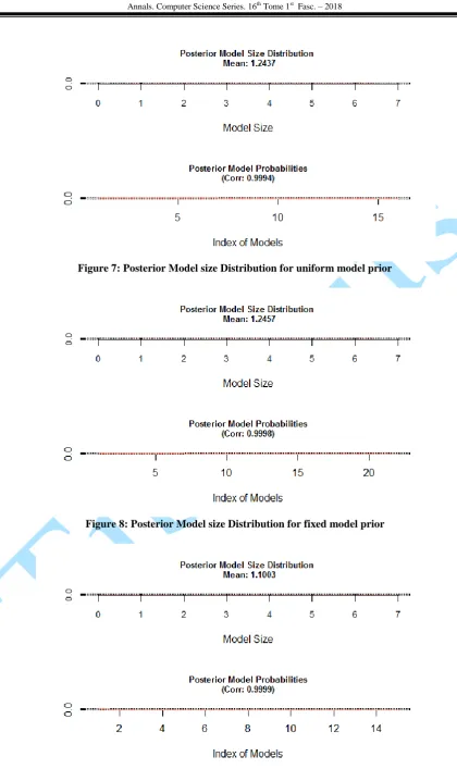
Figure 7: Posterior Model size Distribution for uniform model prior

Figure 8: Posterior Model size Distribution for fixed model prior

(12)

REFERENCES

[Alb07] Albert J. - Bayesian Computation with R, Springer, ISBN 9780-387-71384-7, 2007.

[BB04] Barbieri M. M., Berger J. O. - Optimal predictive model selection, Annals of Statistics, 32, 2004, 870-897.

[BD01] Brock W., Durlauf S. N. - Growth empirics and reality, World Bank Economic Review, 15, 2001, 229-272.

[CG04] Clyde M., George E. I. - Model Uncertainty Statistical Science, 19, 2004, 81-94.

[CCB09] Carney M., Cunningham P., Byrne S. - The benefits of using a complete probability distribution when decision making: an example in anticoagulant drug therapy. Medical Decision Making (forthcoming), 2009.

[CSP96] Clyde M., de Simone H., Parmigiani G. - Prediction Via Orthogonal zed Model Mixing, Journal of the American Statistical Association, 91, 1996, 1197-1208.

[EPR09] Eicher T. S., Papageorgiou C., Raftery A. E. - Determining Growth Determinants: Default Priors and Predictive Performance in Bayesian Model Averaging, Working Paper No. 76, Center for Statistics and the Social Sciences, University of Washington, Seattle, 2009.

[EPR11] Eicher S. T., Papageorgiou C., Raftery A. E. - Default Priors and Predictive Performance in Bayesian Model Averaging, Journal of Applied Econometrics J. Appl. Econ. 26: 30–55, 2011.

[FG94] Foster D. P., George E.I. - The risk inflation criterion for multiple regression. Annals of Statistics 22:1947–1975, 1994.

[FW74] Furnival G. M., Wilson R. W. - Regressions by Leaps and Bounds, Technometrics, 16, 1974, 499-511.

[FLS01a] Fernandez C., Ley E., Steel M. F. J. - Benchmark Priors for Bayesian Model Averaging, Journal of Econometrics, 100, 2001, 381-427.

[FLS01b] Fernandez C., Ley E., Steel M. F. J. - Model Uncertainty in Cross-Country Growth Regressions, Journal of Applied Econometrics, 16, 2001, 563-576.

[Goo52] Good I. J. - Rational decisions. Journal of the Royal Statistical Society, Series B 14: 107–114, 1952.

[GC93] George E. I., McCulloch R. E. - Variable Selection via Gibbs Sampling, Journal of the American Statistical Association, 88, 1993, 881-889.

[GR07] Gneiting T., Raftery A. E. - Strictly proper scoring rules, prediction and estimation. Journal of the American Statistical Association102: 359–378, 2007.

[Her02] Hersbach H. - Decomposition of the continuous ranked probability score for ensembles prediction systems. Weather and Forecasting15: 559–570, 2002.

[HQ79] Hannan E. J., Quinn B. G. - The determination of the order of an autoregression. Journal of the Royal Statistical Society, Series B41: 190–195, 1979.

[H+99] Hoeting J. A., Madigan D., Raftery A. E., Volinsky C. T. – Bayesian Model Averaging: A Tutorial, Statistical Science, 14, 1999, 382-417.

[KW95] Kass R. E., Wasserman L. - A reference Bayesian test for nested hypotheses and its relationship to the Schwarz criterion. Journal of the American Statistical Association90: 928–934, 1995.

[LR92] Levine R., Renelt D. - A sensitivity analysis of cross-country growth regressions, American Economic Review, 82 1992, 942-63.

(13)

[LS09] Ley E., Steel M. F. J. - On the effect of prior assumptions in Bayesian model averaging with applications to growth regression. Journal of Applied Econometrics24(4): 651–674, 2009.

[Mah08] McMahon T. - Ination: 'Causes and effects', In inatioData.com, 2008.

[MR94] Madigan D., Raftery A. E. - Model Selection and Accounting for Model Uncertainty in Graphical Models using Occams Window, Journal of the American Statistical Association, 89, 1994, 1535-1546.

[MS01] Mishkin F. S., Schmidt-Hebbel K. - One Decade of ination Targeting in the world. What do we know and what do we to know?, Central Bank of Chile working paper, No 101, July 2001.

[MW76] Matheson J., Winkler R. - Scoring rules for continuous probability distributions. Management Science22: 1087–1095, 1976.

[MGR95] Madigan D., Gavrin J., Raftery A. E. - Eliciting Prior Information to Enhance the Predictive Performance of Bayesian Graphical Models, Communications in Statistics, Theory and Methods, 24,(1995), 2271-2292.

[OO08] Olubusoye O. E., Oyaromade R. - Ination modelling process in Nigeria. Africa Economic Reseach Consortium, Nairobi, AERC Reseach, Paper 182, 2008.

[OO09] Olubusoye O. E., Okewole D. M. - Prior Sensitivity in Bayesian Linear regression Model, Int. Journal (Sciences), Vol. 3, No. 1, 2009, pp 21-29.

[Raf95] Raftery A. E. - Bayesian Model Selection for Social Research, Sociological Methodology, 25, 1995, 111-163.

[Raf96] Raftery A. E. - Approximate Bayes Factors and Accounting for Model Uncertainty in Generalized Linear Models, Biometrika, 83, 1996, 251-266.

[Raf99] Raftery A. E. - Bayes Factors and BIC: Comment on Weakliem, Sociological Methods and Research, 27, 1999, 411-427.

[RMH97] Raftery A. E., Madigan D., Hoeting J. A. - Bayesian Model Averaging for Linear Regression Models, Journal of the American Statistical Association, 92, 1997, 179-191.

[RPV05] Raftery A. E., Painter I., Volinsky C. T. - BMA: An R package for Bayesian Model Averaging, R News 5, no. 2, 2005, 2-8.

[R+09] Raftery A. E., Hoeting J. A., Volinsky C. T., Painter I., Yeung K. Y. -BMA: An R package for Bayesian Model Averaging, http://cran.r-project.org/web/packages/BMA/, 2009.

[Sal97a] Sala-I-Martin X. - I Just Ran Two Million Regressions, AEA Papers and Proceedings, 87, 1997, 178-183.

[Sal97b] Sala-I-Martin X. - I have just run four million regressions, unpublished typescript, Economic Department, Columbia University, 1997.

[Sel95] Selia F. L. - The Dynamics of Ination in Lesotho, Unpublished M.A. Thesis, University College, Dublin, 1995.

[Str71] Strawderman W.-Proper Bayes minimax estimators of the multivariate normal mean: The Annals of Mathematical Statistics 42 (1), 385–388, 1971.

[SDM04] Sala-I-Martin X., Doppelhofer G., Miller M. I. - Determinants of Long-Term Growth: A Bayesian Averaging of Classical Estimates (BACE) Approach, American Economic Review, 94, 2004, 813-835.

[WS00] Weigend A. S., Shi S. - Predicting daily probability distributions of S&P500 returns. Journal of Forecasting19: 375–392, 2000.