R E S E A R C H
Open Access
The modifiable areal unit problem (MAUP) in the
relationship between exposure to NO
2
and
respiratory health
Marie-Pierre Parenteau
†and Michael C Sawada
*†Abstract
Background:Many Canadian population health studies, including those focusing on the relationship between exposure to air pollution and health, have operationalized neighbourhoods at the census tract scale. At the same time, the conceptualization of place at the local scale is one of the weakest theoretical aspects in health
geography. The modifiable areal unit problem (MAUP) raises issues when census tracts are used as neighbourhood proxies, and no other alternate spatial structure is used for sensitivity analysis. In the literature, conclusions on the relationship between NO2and health outcomes are divided, and this situation may in part be due to the selection of an inappropriate spatial structure for analysis. Here, we undertake an analysis of NO2and respiratory health in Ottawa, Canada using three different spatial structures in order to elucidate the effects that the spatial unit of analysis can have on analytical results.
Results:Using three different spatial structures to examine and quantify the relationship between NO2and respiratory morbidity, we offer three main conclusions: 1) exploratory spatial analytical methods can serve as an indication of the potential effect of the MAUP; 2) OLS regression results differ significantly using different spatial representations, and this could be a contributing factor to the lack of consensus in studies that focus on the relation between NO2and respiratory health at the area-level; and 3) the use of three spatial representations confirms no measured effect of NO2exposure on respiratory health in Ottawa.
Conclusions:Area units used in population health studies should be delineated so as to represent thea priori scale of the expected scale interaction between neighbourhood processes and health. A thorough understanding of the role of the MAUP in the study of the relationship between NO2and respiratory health is necessary for research into disease pathways based on statistical models, and for decision-makers to assess the scale at which interventions will have maximum benefit. In general, more research on the role of spatial representation in health studies is needed.
Background
The neighbourhood concept is equivocal. Neighbourhood units are often defined as small-areas that share some pre-defined set of characteristics [1,2]. Neighbourhood defini-tion is an issue in many health studies at the intra-urban level that depend on this geographical concept. In Canada, the neighbourhood has been operationalized as the census tract in several studies [3-9], even if the use of this
geographic unit is questionable. Only a few Canadian stu-dies have specifically operationalized the neighbourhood in the context of health research [10-12]. As a conse-quence, exactly how place is conceptualized at the local scale is one of the weakest theoretical aspects of the way health studies, among others, are currently conducted [13]. The study of the relationship between exposure to criteria pollutants, such as nitrogen dioxide (NO2) and health outcomes is no exception to this problem. Unfortu-nately, few health studies have focused on this issue [14], despite existing literature that demonstrates the feasibility of measuring different levels of association between health and space under different spatial zoning systems [15-18]. * Correspondence: msawada@uottawa.ca
†Contributed equally
Laboratory for Applied Geomatics and GIS Science (LAGGISS), Department of Geography, University of Ottawa, Simard Hall, 60 University, Ottawa, K1N 6N5, Canada
Considering that studies on the relationship between NO2 and health outcomes are divided regarding the role of exposure to NO2on health, it is surprising that the study of the role of spatial representation in the analysis of this relationship has not received more attention.
Standard geographical units from the Canadian Census, especially the census tract, are often used to operationa-lize the neighbourhood concept. This method finds bene-fit in the readily available Census data for this zoning system [19]. In Canada, census tracts are delineated based on optimal population counts, the compactness of the shape, visible boundaries and input from local experts [20]. The census tract boundaries must follow visible fea-tures when possible, but in some cases, they are deli-neated by administrative boundaries and as such census tract definitions can be equivocal [21,22]. Homogeneity in terms of socioeconomic status is not part of the boundary delineation criteria for census tracts or other standard geographical classification levels used in 2006 Canadian Census geography [21,23]. However, neigh-bourhood units may be expected to be homogeneous along those socioeconomic dimensions related to a given health outcome(s) [1]. Consequently, the use of a census tract as a neighbourhood proxy becomes conceptually problematic. From an analytical viewpoint, using census tracts as the only spatial unit of measure is questionable when no other alternative spatial structure is used for sensitivity analysis, in which case, there can be no assess-ment of MAUP effects on results [16,21].
The Modifiable Area Unit Problem (MAUP) can cause differences in the analytical results of the same input data compiled under different zoning systems [16,24,25]. Open-shaw [16] explains that the MAUP is composed of a scale effect and a zoning effect. Herein, we use the term spatial structure to designate a particular combination of scale and zoning within a bounded region. The scale effect arises when the size of the spatial units of measure changes due to spatial aggregation procedures. Differing spatial aggregation schemes affect analytical results on the same dataset. The zoning effect arises when the number of the spatial units of measure remains the same, but chan-ging their relative structure (changes in the unit bound-aries and shape) generates different analytical results [14,26]. According to some authors [23,27], any study about the association between health and place will be influenced by the scale and zoning design used to conduct the study. Generally, the scale effect is recognized as the most troublesome component of the MAUP, while the zoning effect (effect of unit shape) matters to a lesser extent [23,25]. However, the interplay between zoning and scale is complex because either effect can vary in weight due to the spatial scale of the process(es) being analyzed.
The MAUP impacts the results of univariate and multi-variate regressions [25]. The MAUP can negatively affect
regression model calibration and lead to unreliable results [26]. Some authors have provided insights as to the cause of the MAUP in regression analysis [28]. Accordingly, the MAUP“may be caused by the spatial non-stationarity of multiple predictors that together may be factors for a response variable” [29]. Because the health status of an individual is the result of multiple fac-tors that vary at different spatial scales across a geo-graphic region, health studies are at increased risk of being affected by the MAUP [29,30]. One way to mitigate the impact of the MAUP on analytical results is to create a geographical structure with zoning units that possess “high internal homogeneity”and maintain a considerable amount of external or between-unit heterogeneity [31]. Such mitigation can also represent a solution to errors in the model building process that are induced by positive spatial autocorrelation [32]. Another proposed solution requires the evaluation of the association under different spatial structures (varying zoning and scale) as a way to conduct sensitivity analysis [26].
An automated zone design methodology was first devel-oped for the study of zoning and scale effects on various analytical results [15]. These automated approaches, based on computer algorithms, regroup a set of spatial units into a number of zones so that each unique spatial unit is linked to one zone only [15,33]. A contiguity/adjacency constraint is often used in these models [15]. Examples of other constraints include the compactness (shape), popu-lation count, area size and internal homogeneity. Auto-mated zoning has been used for the study of the relationship between morbidity and deprivation [27]. Results of such experiments indicate that automatically delineated zoning systems that increase spatial aggregation tend to produce stronger correlations over smaller census zones [27]. Observations of increasing strength of statisti-cal relationships with increasing spatial aggregation verify the work of Openshaw [15].
Since the main objective of this research is to determine the impact of the MAUP on the study of the relationship between exposure to NO2and respiratory health, three dif-ferent spatial structures are incorporated into our frame-work: First, census tracts from the 2006 Canadian Census of population are used as small-scale basic administrative units; second, coarser natural neighbourhoods are deli-neated based on a homogeneity criteria in order to repre-sent an optimal zoning design for the socioeconomic processes under consideration, and; third, an automated zoning structure is created through a continuity based aggregation of census tracts in order to present a different zoning structure with a scale equivalent to the natural neighbourhoods. By comparing analytical results from three spatial structures, we will improve our understanding of how scale and zoning influence the measured relation-ship between NO2and health.
Parenteau and SawadaInternational Journal of Health Geographics2011,10:58 http://www.ij-healthgeographics.com/content/10/1/58
Methods
Health Outcome Data
The effect of air pollution on respiratory health can be measured through emergency room visits and hospital admissions [34]. The respiratory morbidity rate for indi-viduals 15 years of age and over from the Ottawa Public Health Unit is the primary health outcome measure in this research.
Health conditions associated with exposure to NO2were identified from the International Classification of Disease 10thRevision (ICD-10) [35] based on literature regarding the health effects of air pollution [36]. All records with a principal diagnosis of chronic lower respiratory disease (codes J40-J47) were selected from theDischarge Abstract Database (DAD) and the National Ambulatory Care Reporting System(NACRS) for fiscal years 2005-2006, 2006-2007 and 2007-2008 and compiled at the geographic level of the census tract and 95 Ottawa neighbourhoods. The Ontario DAD dataset contains“demographic, admin-istrative and clinical data for hospital discharges”and day procedures [37]. NACRS contains“demographic, adminis-trative and clinical data for ambulatory care visits”[38]. Morbidity rates were directly sex and age standardized (45, 48) for age groups 15-24, 25-34, 35-44, 45-54, 55-64, 65-74, 75-84 and 85 and over.
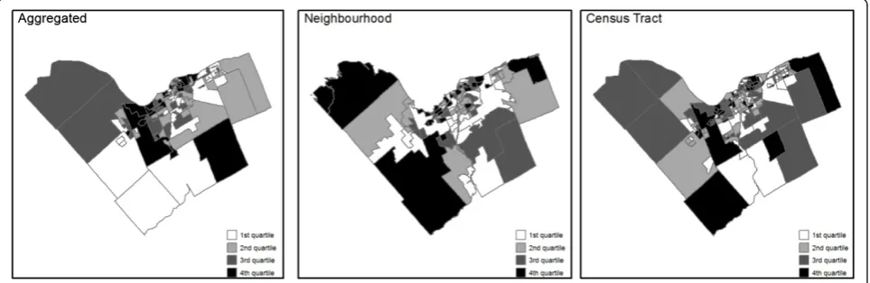
The spatial distributions of theRespiratory health out-come ratefor each of the spatial structures are shown in Figure 1.
Natural neighbourhood, aggregated structure and census tract
The natural neighbourhoods were delineated through a semi-automatic approach with the purpose of being used as the geography of reference for this research as well as for the Ottawa Neighbourhood Study (ONS) project [39]. The objective was to delineate homogeneous units in terms of socioeconomic status (SES), which has been
linked to health outcomes, which would also maximize external heterogeneity. The socioeconomic variables from the 2001 Canadian Census of population that were used in the neighbourhood boundary delineation included:
•Median household income
•Unemployment rate
•Housing affordability
•% Structures built before 1961
•% Dwelling owned
•Median value of dwelling
•% Visible minority
•% Population with a bachelor’s degree
The first step involved automatically aggregating disse-mination areas (DAs) through spatially constrained clus-tering and wombling using the software BoundarySeer [40]. The clustering and wombling algorithms were applied to SES and housing data from the 2001 Canadian Census at the geographic level of the dissemination area (DA),“the smallest standard geographic area for which all census data are disseminated”[41]. Once the automated delineation was completed, the natural neighbourhoods were manually refined. To better represent Ottawa’s neighbourhoods, some boundaries were later updated fol-lowing the release of 2006 Census data. A total of 95 neighbourhood units are within the boundary file. This iterative boundary delineation work was achieved through consultations with the City of Ottawa and leaders of local grassroots organizations and public input. Details on the methodological approach are published elsewhere [39].
The aggregated structure was created through the grouping of census tracts using ArcGIS 9.2 [42] with a simple contiguity constraint. This aggregated set was constructed by first selecting a census tract at random and then unioning it with a neighbour before moving to
the following census tract that was not already part of an aggregated set. This process was repeated until all non-previously aggregated census tracts were visited. We automatically delineated 95 units in total to compare with 95 natural neighbourhoods in order to evaluate the zoning effect. The final spatial structure used in this research is from the 2006 Canadian Census. From the census, 184 census tracts were extracted to cover the study area in order to represent the data and measures at a more detailed spatial scale. The use of these three spa-tial structures allows for the assessment of the scale effect and the zoning effect in the study of the relationship between exposure to NO2and health.
The social, economic and environmental settings where an individual lives are contextual variables in ecological studies that can mediate individual level health [43-46]. The explanatory variables at the geographic level of the census tract, the natural neighbourhood and the aggre-gated structure were obtained from the 2006 Canadian Census of Population. In the case of the data at the geo-graphic level of the neighbourhood, the data were obtained through a custom tabulation from Statistics Canada.
Exposure measures
A land-use regression (LUR) model was developed for the mapping of NO2concentrations in Ottawa, Canada (Figure 2). Details of that model are published elsewhere [47]. The model, which included data on the road net-work, population, green spaces and industrial land-use, yielded an R2 of 0.8055. Zonal statistics within ArcGIS 9.2 were derived from the LUR modelled NO2 layer to derive mean NO2 concentrations for the census tracts, natural neighbourhoods and aggregated structure [48].
Results
Preliminary data analysis was first conducted to determine the role of spatial representation on summary statistics using global spatial autocorrelation and bivariate Moran’s I. Bivariate Ordinary Least Squares (OLS) and multivariate OLS regressions where then applied to the three zoning systems to determine the impact of the MAUP on the relationship between theRespiratory health outcome rate
and exposure to NO2. Spatial regressions were not used in this research because a comparison between spatial regres-sion and OLS has already been explored in another article in preparation by the same authors. SAS (version 9.2) [49] and GEODA [50] were used for statistical and spatial ana-lysis of the data.
Summary statistics
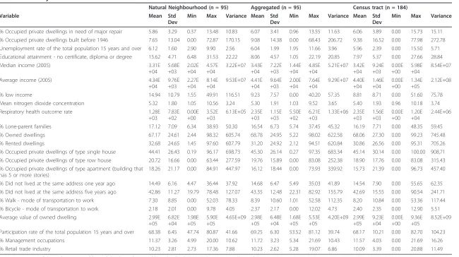
The mean value of the explanatory variables under each of the three spatial structures is similar (Table 1). The vari-ablesEducational attainmentand% low incomehave the highest levels of variability. The variable Mean NO2
concentrationdisplays a much smaller amount of variabil-ity under different spatial structures, with average values ranging from 5.29 to 5.39 ppb. On the other hand, the mean value for theRespiratory health outcome rateis sig-nificantly affected by the use of different spatial structures. The lowest average rate is 1,275.35 per 100,000 at the nat-ural neighbourhood level in comparison to 2,346.89 per 100,000 for the census tract structure. Standard deviations are also similar for most variables under three different spatial structures, but as with the mean values, there are exceptions. Finally, census tracts have higher variance values then the other two spatial structures.
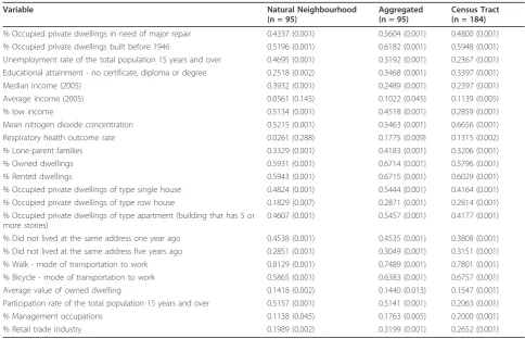
Global spatial autocorrelation
Global Moran’s I spatial autocorrelation statistic mea-sures the self-similarity of a spatial variable’s value as a function of adjacency [51]. Using a first-order Queen’s case spatial weight matrix and 999 permutations, we found statistically significant spatial autocorrelation at a pseudo-significance level ofp≤ 0.05 for all the explana-tory variables for all spatial structures, with the excep-tion of Average income within the natural structure (Table 2). The exposure data (Mean NO2 concentration) is characterized by strong statistically significant spatial autocorrelation under all spatial structures. The Respira-tory health outcome rateexhibits significant spatial auto-correlation within the census and aggregated structures but not within natural neighbourhood boundaries.
The comparison of Moran’s I within the natural neigh-bourhoods and aggregated structure reveals a zoning effect. In general the aggregated structure exhibits higher magnitudes of Moran’s I. For both structures, spatial auto-correlation is statistically significant for all the variables with the exception of theRespiratory health outcome rate
and theAverage income(under the neighbourhood struc-ture). TheRespiratory health outcome rateis characterized by statistically significant positive spatial autocorrelation within the aggregated structure, but not for the natural neighbourhoods.
A scale effect is observed when comparing results using the aggregated structure and census tracts. The aggregated structure, which is based on an aggregation of census tracts, displays stronger spatial autocorrelation in 70% of the variables when compared to the census tract. Whereas, compared to the natural neighbourhoods, global spatial autocorrelation in census tracts is stronger or weaker in half the cases. As such, the use of homogeneous natural neighbourhoods is apparently compensating for the scale effect evident in the aggregated structure that has equiva-lently sized units.
Bivariate Moran’s I
Bivariate Moran’s I is used here in exploratory spatial data analysis (ESDA) to provide information on the
Parenteau and SawadaInternational Journal of Health Geographics2011,10:58 http://www.ij-healthgeographics.com/content/10/1/58
strength of the associations between NO2 concentrations and the other covariates as well as between the Respira-tory health outcome rateand all explanatory variables [52]. This approach also provided preliminary informa-tion on the likely direcinforma-tion of the effect [53].
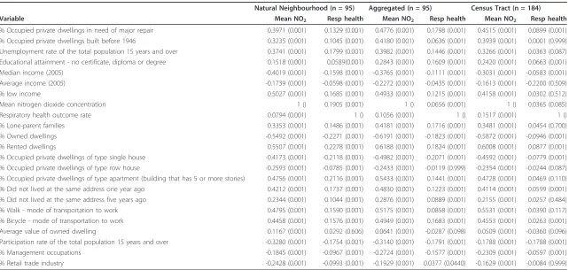
The spatial correlation between theRespiratory health outcome rateand explanatory variables differs from one structure to the other and appears to be affected by scaling and the zoning effects (Table 3). For most relations, the direction or sign of the correlation is the same for all three structures. TheAverage value of owned dwellingand% retail trade industryare two exceptions. TheAverage value of owned dwellinghas a non-significant positive spa-tial correlation with theRespiratory health outcome rate
under the neighbourhood structure, but a negative and non-statistically significant for the aggregated and census tract structures. The% retail trade industryis negatively correlated with theRespiratory health outcome rateunder the natural neighbourhood structure (statistically signifi-cant) and the census tract structure (not statistically signif-icant) but is positive under the aggregated structure (statistically significant).
The strength of correlation between Mean NO2
con-centrationand the Respiratory health outcome rate var-ies according to the spatial structure. For the natural neighbourhoods, bivariate Moran’s I is 0.1905 and is sta-tistically significant. The bivariate Morans’I value for
the same relationship using the aggregated structure is 0.0656 and is statistically significant. Finally, using cen-sus tracts, bivariate Moran’s I value is lowest (I = 0.0365) and not statistically significant.
Bivariate regression
To explore how the scale and zoning affects ordinary least squares, an (OLS) bivariate regression model was developed in GeoDa to measure the relationship between the variableMean NO2 concentrationand the
Respiratory health outcome rate for each of the three spatial structures (Table 4). The measured R2is low for each of the spatial structures: 0.0492 for the census tract structure, 0.0494 for the aggregated structure and 0.0307 with the neighbourhood structure. The value of theMean NO2 concentration coefficient is positive for all three spatial structures; it is statistically significant in the aggregated and the census tract models but not in the natural neighbourhood model.
The OLS regression model of the natural neighbour-hood structure is characterized by a non-normal distribu-tion of the error term (Jarque-Bera) and non-stadistribu-tionarity between the explanatory variables and theRespiratory health outcome rate(Breusch-Pagan and Koenker-Bassett tests). The OLS models for the aggregated and census tract structures are also characterized by a non-normal distribution of the error term (Jarque-Bera) but pass the Figure 2NO2concentrations (ppb) in the study area. Results of the LUR modelling for the mapping of NO2concentrations in Ottawa,
Table 1 Summary statistics
Natural Neighbourhood (n = 95) Aggregated (n = 95) Census tract (n = 184)
Variable Mean Std
Dev
Min Max Variance Mean Std
Dev
Min Max Variance Mean Std
Dev
Min Max Variance
% Occupied private dwellings in need of major repair 5.86 3.29 0.37 13.48 10.83 6.07 3.41 0.96 13.55 11.63 6.06 3.89 0.00 15.73 15.11 % Occupied private dwellings built before 1946 7.65 13.04 0.00 72.87 170.15 9.08 14.38 0.00 68.43 206.72 9.38 16.52 0.00 77.98 272.78 Unemployment rate of the total population 15 years and over 6.12 1.60 2.90 9.90 2.56 6.04 1.99 1.95 11.66 3.96 5.96 2.39 0.00 15.50 5.71 Educational attainment - no certificate, diploma or degree 15.62 4.71 6.48 31.53 22.22 8.06 4.57 1.05 22.19 20.85 7.97 5.37 0.00 27.66 28.84
Median income (2005) 3.31E
+04 5.68E +03 2.02E +04 4.57E +04 3.22E+07 3.43E +04 7.22E +03 1.44E +04 4.85E +04 5.21E+07 3.42E +04 9.24E +03 0.00E +00 5.98E +04 8.54E+07
Average income (2005) 4.34E
+04 9.76E +03 2.27E +04 8.14E +04 9.53E+07 4.41E +04 9.64E +03 2.00E +04 7.64E +04 9.29E+07 4.40E +04 1.46E +04 0.00E +00 1.34E +05 2.12E+08
% low income 14.94 10.79 1.55 49.91 116.51 9.23 7.57 0.00 40.20 57.35 8.81 8.71 0.00 51.60 75.78
Mean nitrogen dioxide concentration 5.32 1.80 1.05 10.56 3.24 5.30 1.91 1.03 9.52 3.65 5.40 1.93 0.96 10.18 3.74
Respiratory health outcome rate 1.28E
+03 7.83E +02 0.00E +00 3.52E +03 6.13E+05 2.35E +03 1.15E +03 5.50E +02 6.21E +03 1.33E+06 2.35E +03 1.56E +03 0.00E +00 1.20E +04 2.44E+06
% Lone-parent families 17.12 7.09 6.34 38.93 50.30 16.54 6.73 5.74 37.45 45.32 16.19 7.71 0.00 48.35 59.45
% Owned dwellings 67.17 24.61 2.44 98.32 605.74 68.78 24.95 5.22 98.02 622.58 68.06 27.30 0.00 99.23 745.48
% Rented dwellings 32.68 24.65 1.45 97.60 607.79 31.20 24.92 2.12 94.51 620.84 30.86 26.56 0.00 95.31 705.26
% Occupied private dwellings of type single house 44.41 26.43 0.19 96.17 698.73 45.30 26.14 0.27 97.35 683.34 45.14 30.14 0.00 100.00 908.71 % Occupied private dwellings of type row house 20.72 16.66 0.00 63.44 277.59 19.76 15.89 0.00 83.08 252.38 18.90 17.76 0.00 83.08 315.43 % Occupied private dwellings of type apartment (building that
has 5 or more stories)
18.26 21.17 0.00 84.91 447.97 16.12 18.44 0.00 73.93 339.92 15.73 21.39 0.00 96.73 457.40
% Did not lived at the same address one year ago 14.49 6.16 4.47 36.44 37.92 14.68 6.47 5.49 35.03 41.89 14.54 7.90 0.00 55.65 62.35 % Did not lived at the same address five years ago 42.86 11.27 19.79 78.48 127.07 43.35 12.48 22.31 82.92 155.79 42.69 15.55 0.00 90.54 241.71 % Walk - mode of transportation to work 7.30 8.85 0.00 52.03 78.33 8.39 10.60 1.01 52.58 112.35 8.20 10.84 0.00 53.36 117.44
% Bicycle - mode of transportation to work 2.18 2.01 0.00 9.78 4.05 2.37 2.17 0.00 12.02 4.73 2.40 2.35 0.00 12.90 5.51
Average value of owned dwelling 2.99E
+05 6.82E +04 1.98E +05 5.90E +05 4.65E+09 2.98E +05 6.48E +04 1.68E +05 5.53E +05 4.20E+09 2.99E +05 9.23E +04 0.00E +00 9.36E +05 8.52E+09
Participation rate of the total population 15 years and over 68.38 6.45 47.74 80.87 41.66 69.25 6.30 53.52 81.12 39.74 68.17 10.21 0.00 82.70 104.23
% Management occupations 11.37 3.26 4.99 20.00 10.62 11.72 3.23 5.34 21.69 10.43 11.57 4.03 0.00 21.69 16.26
% Retail trade industry 10.23 2.81 2.73 17.36 7.88 10.23 2.62 5.28 19.07 6.86 10.09 3.39 0.00 20.88 11.49
Summary statistics of the explanatory variables and the dependent variable under the three spatial structures under study.
tests for stationarity (Breusch-Pagan and Koenker-Bassett). Finally, the census tract and aggregated structures are characterized by statistically significant spatial autocorrela-tion in the residuals using the modified Moran’s I test for regression residuals. Additionally, the R2and adjusted R2 values are smaller for the neighbourhood model than the census tract but according to the log likelihood, Akaike information criterion and the Schwarz criterion the neigh-bourhood model is a better fit.
Multivariate regression
Explanatory variables were introduced into a stepwise regression for each of the three spatial structures using SAS 9.2 to determine the best fitting model for each of the zoning systems (Table 5). Since the objective of this research was to study the effect of the MAUP in the relationship between exposure to NO2 and health, the variableMean NO2 concentrationwas included in each of the models even despite its lack of statistical signifi-cant. All other included variables were statistically significant.
The model developed for the census tract structure contains six explanatory variables:% occupied private dwellings in need of major repairs, % occupied private dwellings built before 1946, Educational attainment,
Average income, % retail trade industryandMean NO2
concentrationand yielded an R2 value of 0.43 and an adjusted R2of 0.41. The model for the aggregated struc-ture is a subset of the census tract model; it contains four of the variables found in the census tract model and explains less of the variability in theRespiratory health outcome rate(R2 = 0.39 and adjusted R2 = 0.37). The model building exercise provided a different set of expla-natory variables using the neighbourhood structure. The model is made up of seven variables (Educational attain-ment, Participation rate of the total population 15 years and over, % management occupations, % walk - mode of transportation to work, % occupied private dwellings of type apartment, % lone-parent families, andMean NO2
concentration). The only common variable to the three models, with the exception ofMean NO2concentration, is Educational attainment. The R2 (0.43) and the adjusted R2(0.38) for the neighbourhood structure lay between the values generated by the OLS models for the census tract and the aggregated structure.
The log likelihood is larger for the natural neighbour-hood than for the census tract and aggregated structures while the AIC and Schwarz criterion have smaller values for the natural neighbourhood structure than the two others, all characterizing the neighbourhood model as Table 2 Global spatial autocorrelation
Variable Natural Neighbourhood
(n = 95)
Aggregated (n = 95)
Census Tract (n = 184)
% Occupied private dwellings in need of major repair 0.4337 (0.001) 0.5604 (0.001) 0.4800 (0.001) % Occupied private dwellings built before 1946 0.5196 (0.001) 0.6182 (0.001) 0.5948 (0.001) Unemployment rate of the total population 15 years and over 0.4695 (0.001) 0.3192 (0.001) 0.2367 (0.001) Educational attainment - no certificate, diploma or degree 0.2518 (0.002) 0.3468 (0.001) 0.3397 (0.001)
Median income (2005) 0.3932 (0.001) 0.2489 (0.001) 0.2397 (0.001)
Average income (2005) 0.0561 (0.145) 0.1022 (0.045) 0.1139 (0.005)
% low income 0.5134 (0.001) 0.4518 (0.001) 0.2859 (0.001)
Mean nitrogen dioxide concentration 0.5215 (0.001) 0.5463 (0.001) 0.6656 (0.001)
Respiratory health outcome rate 0.0261 (0.288) 0.1775 (0.009) 0.1315 (0.002)
% Lone-parent families 0.3329 (0.001) 0.4183 (0.001) 0.3206 (0.001)
% Owned dwellings 0.5931 (0.001) 0.6714 (0.001) 0.5796 (0.001)
% Rented dwellings 0.5943 (0.001) 0.6715 (0.001) 0.6029 (0.001)
% Occupied private dwellings of type single house 0.4824 (0.001) 0.5444 (0.001) 0.4164 (0.001) % Occupied private dwellings of type row house 0.1829 (0.007) 0.2871 (0.001) 0.2814 (0.001) % Occupied private dwellings of type apartment (building that has 5 or
more stories)
0.4607 (0.001) 0.5457 (0.001) 0.4177 (0.001)
% Did not lived at the same address one year ago 0.4538 (0.001) 0.4535 (0.001) 0.3808 (0.001) % Did not lived at the same address five years ago 0.2851 (0.001) 0.3049 (0.001) 0.3151 (0.001)
% Walk - mode of transportation to work 0.8129 (0.001) 0.7489 (0.001) 0.7801 (0.001)
% Bicycle - mode of transportation to work 0.5865 (0.001) 0.6383 (0.001) 0.6757 (0.001)
Average value of owned dwelling 0.1418 (0.002) 0.1440 (0.013) 0.1547 (0.001)
Participation rate of the total population 15 years and over 0.5157 (0.001) 0.5141 (0.001) 0.2063 (0.001)
% Management occupations 0.1138 (0.045) 0.1763 (0.005) 0.2000 (0.001)
% Retail trade industry 0.1989 (0.002) 0.3199 (0.001) 0.2652 (0.001)
Table 3 Bivariate Moran’s I
Natural Neighbourhood (n = 95) Aggregated (n = 95) Census Tract (n = 184)
Variable Mean NO2 Resp health Mean NO2 Resp health Mean NO2 Resp health
% Occupied private dwellings in need of major repair 0.3971 (0.001) 0.1329 (0.001) 0.4776 (0.001) 0.1798 (0.001) 0.4515 (0.001) 0.0899 (0.001) % Occupied private dwellings built before 1946 0.3235 (0.001) 0.1045 (0.001) 0.4180 (0.001) 0.0636 (0.001) 0.3939 (0.001) 0.0001 (0.999) Unemployment rate of the total population 15 years and over 0.3741 (0.001) 0.1799 (0.001) 0.3982 (0.001) 0.1446 (0.001) 0.3266 (0.001) 0.0363 (0.087) Educational attainment - no certificate, diploma or degree 0.1518 (0.001) 0.0589(0.001) 0.2843 (0.001) 0.1609 (0.001) 0.2420 (0.001) 0.0663 (0.001)
Median income (2005) -0.4019 (0.001) -0.1598 (0.001) -0.3765 (0.001) -0.1111 (0.001) -0.3031 (0.001) -0.0583 (0.001)
Average income (2005) -0.1739 (0.001) -0.0598 (0.001) -0.2272 (0.001) -0.0435 (0.001) -0.1613 (0.001) -0.2200 (0.509)
% low income 0.5027 (0.001) 0.1685 (0.001) 0.4933 (0.001) 0.1215 (0.001) 0.4158 (0.001) 0.0302 (0.512)
Mean nitrogen dioxide concentration 1 () 0.1905 (0.001) 1 () 0.0656 (0.001) 1 () 0.0365 (0.085)
Respiratory health outcome rate 0.0794 (0.001) 1 () 0.1056 (0.001) 1 () 0.1517 (0.001) 1 ()
% Lone-parent families 0.3353 (0.001) 0.1486 (0.001) 0.4181 (0.001) 0.1716 (0.001) 0.3481 (0.001) 0.0454 (0.700)
% Owned dwellings -0.5492 (0.001) -0.2271 (0.001) -0.6191 (0.001) -0.1823 (0.001) -0.5872 (0.001) -0.0946 (0.001)
% Rented dwellings 0.5507 (0.001) 0.2278 (0.001) 0.6188 (0.001) 0.1824 (0.001) 0.6008 (0.001) 0.0877 (0.001)
% Occupied private dwellings of type single house -0.4173 (0.001) -0.2118 (0.001) -0.4982 (0.001) -0.2071 (0.001) -0.4592 (0.001) -0.0779 (0.001) % Occupied private dwellings of type row house -0.2593 (0.001) -0.0785 (0.001) -0.2433 (0.001) -0.0119 (0.999) -0.2354 (0.001) -0.0244 (0.087) % Occupied private dwellings of type apartment (building that has 5 or more stories) 0.4756 (0.001) 0.2116 (0.001) 0.5433 (0.001) 0.1441 (0.001) 0.4728 (0.001) 0.0469 (0.110) % Did not lived at the same address one year ago 0.4212 (0.001) 0.1737 (0.001) 0.4830 (0.001) 0.1223 (0.001) 0.4114 (0.001) 0.0599 (0.001) % Did not lived at the same address five years ago 0.2344 (0.001) 0.1044 (0.001) 0.2876 (0.001) 0.0889 (0.001) 0.2155 (0.001) 0.0257 (0.484) % Walk - mode of transportation to work 0.4795 (0.001) 0.1590 (0.001) 0.5175 (0.001) 0.0858 (0.001) 0.5531 (0.001) 0.0390 (0.117) % Bicycle - mode of transportation to work 0.4458 (0.001) 0.1576 (0.001) 0.4949 (0.001) 0.1683 (0.001) 0.4553 (0.001) 0.0263 (0.001)
Average value of owned dwelling 0.1167 (0.001) 0.0292 (0.606) 0.0641 (0.001) -0.0287 (0.098) 0.0509 (0.001) -0.0360 (0.096)
Participation rate of the total population 15 years and over -0.3280 (0.001) -0.1754 (0.001) -0.3140 (0.001) -0.1791 (0.001) -0.1788 (0.001) -0.1788 (0.001)
% Management occupations -0.1845 (0.001) -0.0967 (0.001) -0.2724 (0.001) -0.1577 (0.001) -0.2309 (0.001) -0.0597 (0.001)
% Retail trade industry -0.2428 (0.001) -0.0993 (0.001) -0.1929 (0.001) 0.0377 (0.0440) -0.1629 (0.001) -0.0084 (0.999)
Bivariate Moran’s I values 1) between the explanatory variables and theMean NO2concentration; and 2) between the explanatory variables and theRespiratory health outcome rate.p-values are in parentheses.
Parenteau
and
Sawada
Internation
al
Journal
of
Health
Geographic
s
2011,
10
:58
http://ww
w.ij-healthge
ographics.co
m/content/1
0/1/58
Page
8
of
an improved fit. The model developed under the natural neighbourhood structure is the only one not character-ized by a non-normal distribution of the error term (Jar-que-Bera) and non-stationarity between the explanatory variables and the dependent variables (Breusch-Pagan and Koenker-Bassett tests). In terms of global spatial autocorrelation, only the natural neighbourhood model is not characterized by statistically significant spatial autocorrelation.
Discussion
Numerous studies have concluded that increased expo-sure to NO2 likely contributes to negative respiratory health but no positive and statistically significant associa-tion has been unequivocally found [43,54,55]. The main objective of this research was to examine the role of spa-tial representation, focusing on MAUP effects, in the study of the relationship between exposure to NO2and respiratory health. We find that the outcomes of this exposure/health relation are tied to the MAUP. The MAUP provides a method to learn how scale and zoning may affect the lack of consensus in studies that aim to expose the role that NO2has on overall health outcomes. Some have recommended approaches to gain a better insight into how the MAUP can affect analytical results
[16,56,57] but few published studies have incorporated any of these in their analyses. In our research, we imple-mented two of the recommended approaches [26]. The first approach is based on the use of an optimal zoning proposal, while the second suggests conducting sensitiv-ity analysis using alternate spatial structures. In this study, the natural neighbourhoods delineated through a semi-automated method were used as the“optimal” zon-ing system. As mentioned, the main component of the delineation process was based on the concept of internal homogeneity along socioeconomic dimensions. Neigh-bourhoods were delineated in order to make homoge-neous units in terms of SES. These units may not be suitable for all studies conducted in Ottawa, but they are assumed to represent many social processes associated with health. We also believe that these natural neigh-bourhoods could be used for research examining other health outcomes, aside from respiratory morbidity or even other social processes related to SES.
This research also used sensitivity analysis to mitigate the effect of the MAUP [16,56,57]. This study was con-ducted using three spatial structures: natural neighbour-hoods, an aggregated structure of the same scale as the former but with a different zoning and census tracts with a different scale from the former structures. Using this Table 4 Bivariate regression
Natural Neighbourhood (n = 95) Aggregated (n = 95) Census Tract (n = 184)
Bivariate RESP Bivariate RESP Bivariate RESP
R-squared 0.0307 0.0494 0.0492
Adjusted R-squared 0.0202 0.0392 0.0440
Sum squared residual 55810400.0000 118990000.0000 424291000.0000
Sigma-square 600112.0000 1279470.0000 2330000.0000
S.E. of regression 774.6690 1131.1400 1526.8500
Sigma-square ML 587478.0000 1252530.0000 2305000.0000
S.E of regression ML 766.4710 1119.1700 1518.5300
F-statistic 2.9462 4.8363 9.4154
Prob(F-statistic) 0.0894 0.0303 0.0025
Log likelihood -765.7700 -801.7310 -1608.9800
Akaike 1535.5400 1607.4600 3221.9500
Schwarz criterion 1540.6500 1612.5700 3228.3800
Intercept coefficient 869.8488 (0.0007) 1634.0250 (< 0.0001) 1379.7439 (< 0.0001)
Mean NO2coefficient 76.2276 (0.0894) 134.3078 (0.0303) 179.136 (0.0024)
Jarque-Bera 6.3023 (0.0428) 26.1702 (< 0.0001) 923.152 (< 0.0001)
Breusch-Pagan Test 5.1764 (0.0228) 1.5039 (0.2200) 0.1623 (0.6870)
Koenker-Bassett test 4.1263 (0.0422) 1.0065 (0.3157) 0.0270 (0.8693)
Moran’s I (error) -0.0039 (0.8723) 0.2454 (< 0.0001) 0.1080 (0.0096)
Lagrange Multiplier (lag) 0.0003 (0.9842) 12.2297 (0.0004) 5.4663 (0.0193)
Robust LM (lag) 0.0112 (0.9155) 0.1264 (0.7221) 0.0668 (0.7959)
Lagrange Multiplier (error) 0.0025 (0.9599) 1.0239 (0.3115) 5.4253 (0.0198)
Robust LM (error) 0.0133 (0.9079) 13.2537 (0.0013) 0.0257 (0.8724)
Results of the bivariate regressions (OLS) between theMean NO2concentration(mean NO2) and theRespiratory health outcome rate(RESP) for the three spatial
Table 5 Multivariate regression
Natural Neighbourhood (n = 95) Aggregated (n = 95) Census Tract (n = 184)
Multivariate OLS Multivariate OLS Multivariate OLS
R-squared 0.4306 0.3947 0.4341
Adjusted R-squared
0.3848 0.3678 0.4150
Sum squared residual
32783700.0000 576190000000.0000 252486000.0000
Sigma-square 376824.0000 841798.0000 1426470.0000
S.E. of regression
613.8600 917.4960 1194.3500
Sigma-square ML
345091.0000 797493.0000 1372210.0000
S.E of regression ML
587.4450 893.0250 1171.4100
F-statistic 9.3999 14.6759 22.6379
Prob(F-statistic) 0.0000 0.0000 0.0000
Log likelihood -740.4980 -780.2880 -1561.2200
Akaike 1497.0000 1570.5800 3136.4400
Schwarz criterion
1517.4300 1583.3400 3158.9500
Variables n.a. n.a. n.a.
Intercept 5327.4610 (0.0001) Intercept 738.3682 (0.0192) Intercept -1013.495 (0.0905) Mean NO2concentration -18.0183
(0.6855)
Mean NO2concentration 36.4373 (0.5349) Mean NO2concentration 30.9425 (0.5706)
Educational Attainment 78.4534 (0.0002)
% Occupied private dwellings in need of major repairs 179.7687 (0.0007)
% Occupied private dwellings in need of major repairs 177.3213 (< 0.0001) Participation Rate -53.0824 (0.0003) % Occupied private dwellings built before
1946 -29.6505 (0.0118)
% Occupied private dwellings built before 1946 -20.91902 (0.0163)
% Management occupations -84.1282 (0.004)
Educational Attainment 73.4928 (0.0111) Educational Attainment 113.1868 (< 0.0001)
% Walk - mode of transportation to work 40.1355 (< 0.0001)
Average income 0.0151 (0.0442)
% Occupied private dwellings of type apartment -16.7916 (0.0015)
% Retail trade industry 73.8654 (0.0161)
% Lone-parent families -34.7820 (0.0157)
Jarque-Bera 0.9239 (0.6300) 44.1697 (< 0.0001) 1173.241 (< 0.0001)
Breusch-Pagan Test
3.0898 (0.8765) 8.5867 (0.0723) 149.1566 (< 0.0001)
Koenker-Bassett test
3.1269 (0.8730) 3.8557 (0.4258) 21.8956 (0.0012)
Moran’s I (error)
0.0498 (0.2527) 0.1892 (0.0006) 0.1091 (0.0051)
Lagrange Multiplier (lag)
0.1953 (0.6584) 7.8384 (0.0051) 2.7432 (0.0976)
Robust LM (lag)
3.4593 (0.0628) 0.6030 (0.4374) 0.2288 (0.6324)
Lagrange Multiplier (error)
0.4047 (0.0554) 7.8074 (0.0052) 5.5355 (0.0186)
Robust LM (error)
3.6687 (0.0628) 0.5720 (0.4494) 3.0211 (0.0821)
Results of the multivariate regressions (OLS) for the three spatial structures under study.p-values are in parentheses.
Parenteau and SawadaInternational Journal of Health Geographics2011,10:58 http://www.ij-healthgeographics.com/content/10/1/58
sensitivity analysis method allowed us to address a num-ber of questions related to the effect that the MAUP has on spatial autocorrelation and hence on univariate and bivariate and regressions.
Exploratory and confirmatory data analysis methods were used to assess the role of spatial representation in the study of the relationship between exposure to NO2 and the respiratory health outcomes. The results obtained from the different analytical approaches con-verge towards three main conclusions, which will be dis-cussed in more detail:
1. Exploratory analytical methods, such as univariate Moran’s I and bivariate Moran’s I, can serve as an indication of the potential effect of the MAUP in the study of the relationship between exposure to NO2 and health;
2. Bivariate and multivariate regressions suggest that different spatial representations can contribute to the lack of consistency of previous literature regarding the relationship between exposure to NO2and health; 3. Results from all three different spatial representa-tions confirm no significant effect of NO2 exposure on respiratory health in Ottawa that is not due to unreasonable spatial units of measurement.
The results obtained confirm the documented effect of the MAUP [58,59] on summary statistics. The analysis of the summary statistics demonstrates that the MAUP does not have a strong effect on the mean of explanatory vari-ables, confirming the previous results of other researchers [26]. Our results further substantiate the work of those authors who observed that the variance decreases with increasing aggregation. Likewise, we observe that the var-iance is affected when the same number of spatial units of study are used but with a different partitioning or zoning of space.
Global Moran’s I was calculated for all the explanatory variables as well as for the dependent variable within three spatial structures. All the explanatory variables were characterized by positive spatial autocorrelation within the three zoning systems. Moran’s I values tend to be lower for census tracts than the other two spatial structures. As aggregation increases, Moran’s I is also expected to increase due to the“increased homogeneity in the landscape structure” [26]. While not definitive, our results concur.
The dependent variableRespiratory health outcome ratedisplays low levels of statistically significant spatial autocorrelation using census tracts and the aggregated structure. Using natural neighbourhoods, global Moran’s I calculated for the dependent variable, reveals a non-significant value close to zero. In this case, instead of spatial autocorrelation increasing with aggregation, it is
no longer statistically significant. By way of explanation, the natural neighbourhoods are internally homogeneous in terms of SES and adequately depict the spatial scale of the Respiratory health outcome rate, thus reducing spatial dependence between neighbourhoods. A zoning effect is also observed; levels of spatial autocorrelation using the natural neighbourhood structure are reduced when compared to the aggregated structure. These observations serve as a rationale for using custom geo-graphy delineated using processes knowna priorito be associated with the dependent health outcome variable of interest.
Under the MAUP, we expected both the aggregated and neighbourhood structures (n = 95) to be character-ized by stronger bivariate Moran’s I values between the explanatory variables and theMean NO2 concentration then under the census tract structure (n = 184) because aggregation is known to increase the strength of correla-tion [16,27]. The use of an optimal zone design in the natural neighbourhoods based on minimizing internal homogeneity appears to be reducing the scale effect of the MAUP. For half of the explanatory variables, the cor-relation withMean NO2concentrationis stronger at the census tract level than at the neighbourhood level orvice versa. On the other hand, the correlations measured using the aggregated structure are stronger (70% of the variables have stronger correlation) than under the cen-sus tract structure, which is the expected result [16]. Moreover, a relatively strong zoning effect is observed when comparing the bivariate Moran’s I values for the correlation between NO2and health for the neighbour-hood and aggregated structures. Similar results were obtained for the correlations between the explanatory variables and theRespiratory health outcome rate. This confirms that the natural neighbourhoods, which are internally homogeneous from a socioeconomic perspec-tive, better capture the processes linked to respiratory health outcomes. We also found that the variable% retail trade industryhas changed directions depending on the spatial structure, confirming that“correlation inference is not robust to the aggregation process”[60].
The use of an exploratory analytical approach in the context of sensitivity analysis can be seen as a tool to assess the role of the MAUP prior to conducting confir-matory data analysis. Exploratory analysis allowed us to obtain a more in-depth understanding of the potential effect of the MAUP on the results of statistical modeling used in the study of the relationships between area-level health and other variables [61].
and the dependent variable once again confirmed both the zoning effect and the scale effect of the MAUP. According to the census tract and aggregated structures, there is a low but statistically significant relationship betweenMean NO2concentrationandRespiratory health
outcome rate. As expected from earlier work on the MAUP, the R2value is higher when using an aggregated structure (coarser level of aggregation) then with the cen-sus tract [29]. The relationship measured between NO2 andRespiratory health outcome ratecannot be confirmed using the neighbourhood structure in this study as it is not statistically significant. The OLS model for the neigh-bourhood structure is the only model not characterized by statistically significant positive spatial autocorrelation in the residuals and passes all tests for non-normality of the error term and heteroskedasticity, suggesting this model is correctly fitted.
The effect of the MAUP on multivariate analyses has been described as “complex and unpredictable” [26]. Considering that the health of an individual is the result of various factors apart from exposure to NO2[62], the relationship is difficult to measure. The question of which variables are significant within our multivariate regression models is an essential element to be addressed; there was only one variable common to all three models (aside fromMean NO2concentrationwhich was forced into the models). The variableEducational attainmentis an explanatory variable for variations in the morbidity rate for all three structures. In other words, scale and/or the zoning design considerations that may mediate this variable’s inclusion/exclusion are being filtered out. The geographic scale of the variableEducational attainment
is probably larger than the scale of the census tract. Another comparison to be made is between the variables used as input into the delineation of the optimal zoning design and the variables included in the different models. We observe that the census tract model includes both% occupied private dwellings built before 1946andAverage income, which were used in the delineation of the natural neighbourhoods. By creating an optimal zoning system based on these variables and other SES variables, housing and income covariates are no longer confounding vari-ables in the relationship between exposure to NO2 and health and hence are not found in the neighbourhood model.
The variableMean NO2concentrationis not a statisti-cally significant factor in any model and so allowed other variables to express their association with respiratory health. For example,% Lone-parent families, a measure of the economic structure, is part of the optimal zoning design model based on the natural neighbourhoods but not the census tract or aggregated structures. If the pro-cess of aggregation has the same impact on dependent and independent variables, then the effect of the MAUP
is reduced in severity [25]. These results are demon-strated when the independent and dependent variables are spatially autocorrelated and averaged. Since the level of global spatial autocorrelation was found to be different for the dependent variable as a function of the spatial structure, the differences observed between the models are justified. Among the variables included in the neigh-bourhood model, two variables have a coefficient with a direction opposite to that suggested by bivariate Moran’s I (Mean NO2concentrationand% Lone-parent families). Finally, the resemblance between the census tract and the aggregated structure; the aggregated structure is a complete subset of the census tract model. Aggregation can potentially generate collinearity between independent variables [29].
The MAUP implies that an OLS model developed using a specific spatial structure should not be trans-ferred to another spatial structure with the same expecta-tions. This finding has implications for research that may use index mapping techniques to estimate community vulnerability to air pollutants. Moreover, this finding has significant implications for studies that aim to propose morbidity pathways using variables that are found to be significant in models tested at only one scale. Thus, there is the prospect that different scales of analysis will deliver markedly different sets of explanatory variables induced by the MAUP. The sensitivity analysis conducted in this research clearly demonstrates that the explanatory factors of respiratory health will vary according to the geographi-cal structure used to conduct the study. Since research relating exposure to NO2 and health uses a variety of geographical units to conduct the analysis, the variability of the results of previous research may be caused by the MAUP. We believe the delineation of a custom geogra-phy that coincides with the spatial scale of the phenom-enon under investigation can be justified because there is no prior reason to believe that administrative and statisti-cal boundaries reflect the fundamental nature and sstatisti-cale of the economic and social phenomena measured within them [25]. The use of optimal zoning designs, like our natural neighbourhoods, becomes a way to resolve the consequences of geographic and methodological scale, the former describing the geography used to identify social processes and the latter the scale of data collection and aggregation [63].
The use of three different spatial representations con-firms no measurable effect of NO2exposure on respira-tory health in Ottawa. Under all three spatial structures, bivariate OLS regression between theMean NO2
concen-trationand theRespiratory health outcome ratesuggests that no significant relation is present. Based on the results obtained, we can confirm that in Ottawa, the lack of a significant statistical association is probably not induced by the use of a particular geography. The use of
Parenteau and SawadaInternational Journal of Health Geographics2011,10:58 http://www.ij-healthgeographics.com/content/10/1/58
sensitivity analysis allows us to validate and conclude that the strength of the measured relationship is not produced by neighbourhood boundaries poorly reflecting“the eco-logical properties that shape”health processes [64].
Our methodological approach demonstrates that many factors could explain the observed differences in tory morbidity rates in Ottawa. Considering that respira-tory health has already been associated with SES in several studies [65], our research serves as another example of the importance of the social and the envir-onmental context on health.
There have been few studies on the role of spatial representation in air quality and health. To our knowl-edge, this is the first study specifically interested in the effect of scale and zoning on the relationship between exposure to NO2and health. However, our observations do agree with previous research on the subject. Of the limited research on the issue of scale and zoning, others have concluded that“the use of different specifications to assess spatial concentration, agglomerations economies, and trade determinants produces substantial variation in the estimated coefficients”[25]. A study on the relation between morbidity and deprivation showed that the use of spatial representations other than the census tract pro-duced different analytical results [27]. On the other hand, some suggest that the method of neighbourhood defini-tion does not significantly alter reladefini-tionships and their strength [2,11]. Additional studies on the impact of using different conceptualizations of the neighbourhood on analytical results are required to understand the role of spatial representation. In return, a thorough understand-ing of the role of MAUP on the study of the relationship between NO2concentration and health will allow deci-sion-makers to develop interventions where they are the most needed. Policy makers’ decision about how to improve the health of communities should be strongly influenced by the conclusions that neighbourhood quality affects health. This is particularly of interest in Canada where the population at large believes that the govern-ment has a responsibility for the health of citizens [66].
The use of an optimal zone design that has been reviewed and approved by city planners, public health practitioners, community health and resource persons as well as representatives from grassroots organizations is a strength of this research. These natural neighbourhood units have also been used for the Ottawa Neighbourhood Study (http://www.neighbourhoodstudy.ca) and have been updated since their production to reflect changes in Otta-wa’s communities. Another strong point of this research is the use of an automated zone design to create an aggre-gated structure that we could use to compare to the cen-sus tract structure and our natural neighbourhoods. However, our aggregated structure had to be created by grouping census tracts because of the availability of health
data at that geographic level. As a consequence, we did not have as much flexibility when creating the aggregated structure as would be available if a smaller geographic set was used as the basic spatial unit for reporting census and health data. Moreover, our aggregation method produced a single boundary realization that is one of a finite number of possibilities when using a random seeding method that begins with a fixed tessellation defined by census tracts. Future work could provide tools to exhaust all possible aggregations and generate empirical frequency distribu-tions of statistical estimates that could be used to evaluate the sensitivity of results to aggregation effects. Another feature that makes this study more complicated to admin-ister is the fact the NO2concentration is not a statistically significant explanatory variable in the multivariate regres-sions. If the circumstances were different, we would have a better insight into how NO2’s association with respiratory health varies at different scales. Finally, as a cross-sectional type study, we were limited in having only a few weeks of atmospheric sampling and our results do not preclude the future research with more environmental data through time from coming to different conclusions on the NO2/ Health connection on Ottawa.
Conclusions
The natural neighbourhoods used in this research can be viewed as“exposure areas”as they were delineated with the objective of creating homogeneous units from an SES perspective [67]. The use of area level data such as income, education and housing variables from the Canadian Cen-sus created units where environmental and social condi-tions are equivalent. There is increasing evidence that neighbourhood context affects the health of individuals living therein [68] and it is not unreasonable to assume that an appropriate delineation of neighbourhoods is essential to research outcomes and recommendations that may arise from such studies. Area units should be deli-neated with the purpose of representing the expected rela-tionship between neighbourhood and health. If this relationship is well defined, the modifiable area units are not a problem [31]. This research confirms the conclu-sions of previous studies that more research on the role of spatial representation in health studies in general.
List of abbreviations
Abbreviations include in the manuscript include the AIC: Akaike Information Criterion; DA: Dissemination area; AD: Discharge Abstract Database; ESDA: Exploratory spatial data analysis; LUR: Land-use regression; MAUP: Modifiable Area Unit Problem; MOHLTC: Ministry of Health and Long-Term Care; NACRS: National Ambulatory Care Reporting System; NO2- Nitrogen dioxide; OLS:
Ordinary Least Squares; ONS: Ottawa Neighbourhood Study; SES: Socioeconomic status
Acknowledgements
developing the natural neighbourhoods. The authors would like to thank Natividad Urquizo from the Community Sustainability Department, City of Ottawa, for providing the air quality data.
Authors’contributions
MPP performed the statistical analysis and drafted the manuscript. MCS programmed the automated zone design system and critically revised the manuscript for important intellectual content. All authors contributed equally to the study design, read and approved the final manuscript. This research is a contribution to the Ottawa Neighbourhood Study (http://www.
neighbourhoodstudy.ca) and the authors thank all those involved in its inception and continuance, including funders.
Competing interests
The authors declare that they have no competing interests.
Received: 1 August 2011 Accepted: 31 October 2011 Published: 31 October 2011
References
1. Galster GC:On the nature of neighbourhood.Urban Studies2001,
38:2111-2124.
2. Jones AP, van Sluijs EMF, Ness AR, Haynes R, Riddoch CJ:Physical activity in children: does how we define neighbourhood matter?Health & Place 2010,16:236-241.
3. Buzzelli M, Jerrett M, Burnett R, Finklestein N:Spatiotemporal perspectives on air pollution and environmental justice in Hamilton, Canada, 1985-1996.Annals of the Association of American Geographers2003,93:557-573. 4. Glazier RH, Bradley EM, Gilbert JE, Rothman L:The nature of increased
hospital use in poor neighbourhoods: Findings from a Canadian inner city.Canadian Journal of Public Health2000,91:268-273.
5. James PD, Wilkins R, Detsky AS, Tugwell P, Manuel DG:Avoidable mortality by neighbourhood income in Canada: 25 years after the establishment of universal health insurance.Journal of Epidemiology and Community Health2007,61:287-296.
6. Gauvin L, Robitaille E, Riva M, McLaren L, Dassa C, Potvin L:
Conceptualizing and operationalizing neighbourhoods.Canadian Journal of Public Health2007,98:S18-S26.
7. Walks RA, Maaranen R:Gentrification, social mix, and social polarization: Testing the linkages in large Canadian cities.Urban Geography2008,
29:293-326.
8. Généreux M, Auger N, Goneau M, Daniel M:Neighbourhood
socioeconomic status, maternal education and adverse birth outcomes among mothers living near highways.Journal of Epidemiology and Community Health2008,62:695-700.
9. Urquia ML, Frank JW, Glazier RH, Moineddin R, Matheson FI, Gagnon AJ:
Neighborhood context and infant birthweight among recent immigrant mothers: A multilevel analysis.American Journal of Public Health2009,
99:285-293.
10. Luginaah IN, Jerrett M, Elliott S, Eyles J, Parizeau K, Birch S, Abernathy T, Veenstra G, Hutchinson B, Giovis C:Health Profiles of Hamilton: Spatial Characterisation of Neighbourhoods for Health Investigations.GeoJournal 2001,53:135-147.
11. Ross NA, Tremblay S, Graham K:Neighborhood influences on health in Montreal, Canada.Social Science & Medicine2004,59:1485-1494. 12. Drackley A, Newbold KB, Taylor C:Defining Socially-Based Spatial
Boundaries in the Region of Peel, Ontario, Canada.International Journal of Health Geographics2011,10:38.
13. Matthews SA:The salience of neighbourhood; some lessons from sociology.Am J Prev Med2008,34:257-259.
14. Stafford M, Duke-Williams O, Shelton N:Small are inequalities in health: are we underestimating them?Social Science & Medicine2008,
67:891-899.
15. Openshaw S:A geographical solution to scale and aggregation problems in region-building, partitioning and spatial modelling.Transactions of the Institute of British Geographers1977,2:459-472.
16. The modifiable areal unit problem. [http://qmrg.org.uk/files/2008/11/38-maup-openshaw.pdf].
17. Holt D, Steel DG, Tranmer M:Area homogeneity and the modifiable areal unit problem.Geographical Systems1996,3:181-200.
18. Reynolds H, Amrhein C:Using a spatial data set generator in an empirical analysis of aggregation effects on univariate statistics.Geographical and Environmental Modelling1997,1:199-219.
19. Gauvin L, Riva M, Barnett T, Richard L, Craig CL, Spivock M,et al:
Association between neighborhood active living potential and walking.
American Journal of Epidemiology2008,167:944-953.
20. Statistics Canada - Census tract: Detailed Definition.[http://geodepot. statcan.gc.ca/2006/180506051805140305/03150707/
121514070405190318091620091514_05-eng.jsp? REFCODE=10&LANG=E&GEO_LEVEL=12&TYPE=L].
21. Lee BA, Reardon SF, Firebaugh G, Farrell CR, Matthews SA, O’Sullivan D:
Beyond the census tract: patterns of determinants of racial segregation at multiple geographic scales.American Sociological Review2008,73:766-791. 22. Schaefer-McDaniel N, O’Brien Caughy M, O’Campo P, Gearey W:Examining
methodological details of neighbourhood observations and the relationship to health: a literature review.Social Science & Medicine2010,
70:277-292.
23. Schuurman N, Bell N, Dunn JR, Oliver L:Deprivation indices, population health and geography: an evaluation of the spatial effectiveness of indices at multiple scales.Journal of Urban Health: Bulletin of the New York Academy of Medicine2007,84:591-603.
24. Riva M, Gauvin L, Apparicio P, Brodeur JM:Disentangling the relative influence of built and socioeconomic environments on walking: the contribution of areas homogeneous along exposures of interest.Social Science & Medicine2009,69:1296-1305.
25. Briant A, Combes PP, Lafourcade M:Dots to boxes: do the size and shape of spatial units jeopardize economic geography estimations?Journal of Urban Economics2010,67:287-302.
26. Jelinski DE, Wu J:The modifiable areal unit problem and implications for landscape ecology.Landscape Ecology1996,11:129-140.
27. Cockings S, Martin D:Zone design for environment and health studies using pre-aggregated data.Social Science & Medicine2005,60:2729-2742. 28. Fotheringham AS, Brunsdon C, Charlton ME:Geographically weighted
regression: the analysis of spatially varying relationshipsUnited Kingdom: Wiley; 2002.
29. Swift A, Liu L, Uber J:Reducing MAUP bias of correlation statistics between water quality and GI illness.Computers, Environment and Urban Systems2008,32:134-148.
30. Diniz-Filho JAF, Nabout JC, Telles MP, Soares TN, Rangel TFLVB:A review of techniques for spatial modeling in geographical, conservation and landscape genetics.Genetics and molecular Biology2009,32:203-211. 31. Haynes R, Daras K, Reading R, Jones A:Modifiable neighbourhood units,
zone design and residents’perceptions.Health & Place2007,13:812-825. 32. Mu L, Wang F:A scale-space clustering method: mitigating the effect of
scale in the analysis zone-based data.Annals of the Association of American Geographers2008,98:85-101.
33. Daras K, Alvanides S:Zone design in public health policy.InGIS for sustainable development.Edited by: Campagna M. United Kingdom: Taylor 2006:247-265.
34. Lee D, Ferguson C:Air pollution and health in Scotland: a multicity study.Biostatistics2009,10:409-423.
35. Canadian Institute for Health Information:International statistical classification of diseases and related health problems, tenth revision, Canada. CIHI (2006) ICD-10-CA/CCI2006.
36. Kampa M, Castanas E:Human health effects of air pollution.Environmental Pollution2008,151:362-367.
37. Discharge Abstract Database.[http://www.cihi.ca/CIHI-ext-portal/internet/ en/document/types+of+care/hospital+care/acute+care/services_dad]. 38. National Ambulatory Care Reporting System.
[http://www.cihi.ca/CIHI-ext-portal/internet/EN/TabbedContent/types+of+care/hospital+care/emergency +care/cihi016745].
39. Parenteau M-P, Sawada M, Kristjansson EA, Calhoun M, Leclair S, Labonté R, et al:Development of neighborhoods to measure spatial indicators of health.URISA Journal2008,20:43-55.
40. BoundarySeer [Computer Software]. Ann Harbor, MI: Terraseer. 41. Statistics Canada - Dissemination Area (DA): Detailed Definition.[http://
www12.statcan.ca/census-recensement/2006/ref/dict/geo021-eng.cfm]. 42. ArcGIS (version 9.2) [Computer software]. Redlands, CA: ESRI. 43. Sahsuvaroglu T, Jerrett M, Sears MR, McConnell R, Finkelstein N, Arain A,
Newbold B, Burnett R:Spatial analysis of air pollution and childhood Parenteau and SawadaInternational Journal of Health Geographics2011,10:58
http://www.ij-healthgeographics.com/content/10/1/58
asthma in Hamilton, Canada: comparing exposure methods in sensitive subgroups.Environmental Health2009,8:1.
44. Jerrett M, Finkelstein M:Geographies of risk in studies linking chronic air pollution exposure to health outcomes.Journal of Toxicology and Environmental Health Part A2005,68:1207-1242.
45. Diez-Roux AV:A glossary for multilevel analysis.Journal of Epidemiology and Community Health2002,56:588-594.
46. Piro FN, Madsen C, Naess O, Nafstad P, Claussen B:A comparison of self reported air pollution in people with and without chronic diseases.
Environmental Health2008,7:1.
47. Parenteau M-P, Sawada MC:The role of spatial representation in the development of a LUR model for Ottawa, Canada.Air Quality, Atmosphere and Health2010, 1-13.
48. Hu Z, Rao KR:Particulate air pollution and chronic ischemic heart disease in the eastern United States: a county level ecological study using satellite aerosol data.Environmental Health2009,8:1.
49. SAS Institute Inc. (version 9.2) [Computer software]. Cary. NC: SAS Institute INC.
50. Anselin L, Syabri I, Kho Y:GeoDa: An introduction to spatial data analysis.
Geographical Analysis2006,38:5-22.
51. Anselin L:Spatial statistical modeling in a GIS environment.InGIS, spatial analysis, and modelling.Edited by: Maguire D, Batty M, Goodchild MF. Redlands: ESRI Press; 2005:93-111.
52. Sridharan S, Tunstall H, Lawder R, Mitchell R:An exploratory spatial data analysis approach to understanding the relationship between deprivation and mortality in Scotland.Social Science & Medicine2007,
65:1942-1952.
53. Henderson SB, Beckerman B, Jerrett M, Brauer M:Application of land use regression to estimate long-term concentrations of traffic-related nitrogen oxides and fine particulate matter.Environmental Science & Technology2007,41:2422-2428.
54. Villeneuve PJ, Chen L, Stieb D, Rowe BH:Associations between outdoor air pollution and emergency department visits for stroke in Edmonton, Canada.European Journal of Epidemiology2006,21:689-700.
55. Clark NA, Demers PA, Karr CJ, Koehoorn M, Lencar C, Tamburic L, Brauer M:
Effect of early life exposure to air pollution on development of childhood asthma.Environmental Health Perspectives2010,118:284-290. 56. Openshaw S, Taylor PJ:The modifiable areal unit problem.InQuantitative
geography: a British view.Edited by: Wrigley N, Bennett R. United Kingdom: Routledge 1981:60-69.
57. Fotheringham AS:Scale-independent spatial analysis.InAccuracy of spatial databases.Edited by: Goodchild M, Gopal S. United Kingdom: Taylor 1989:221-228.
58. Arbia G:Spatial data configuration in statistical analysis of regional economic and related problemsNetherlands: Kluwer Academic Publishers; 1989. 59. Amrhein CG, Reynolds H:Using the Getis statistic to explore aggregation
effects in metropolitan Toronto census data.The Canadian Geographer 1997,41:137-149.
60. Fotheringham AS, Wong DWS:The modifiable area unit problem in multivariate analysis.Environment and Planning A1991,23:1025-1044. 61. Waller LA, Gotway CA:Applied spatial statistics for public health dataUSA:
Wiley; 2004.
62. Goovaerts P:Geostatistical analysis of county-level lung cancer mortality rates in the southeastern United States.Geographical Analysis2010,
42:32-52.
63. Reardon SF, Matthews SA, O’Sullivan D, Lee BA, Firebaugh G, Farrell CR, Bischoff K:The geographic scale of metropolitan racial segregation.
Demography2008,45:489-514.
64. Sampson RJ, Morenoff JD:Spatial (dis) advantage and homicide in Chicago neighborhoods.InSpatially integrated social science.Edited by: Goodchild M, Janelle D. New York: Oxford University Press; 2004:145-170. 65. McElmurry B, Buseh A, Dublin M:Health education program to control asthma in multiethnic, low-income urban communities: the Chicago health corps asthma program.Chest1999,116:198S-199S.
66. Heyman J, Fisher A:Neighbourhoods, health research, and its relevance to public policy.InNeighbourhoods and Health.Edited by: Kawachi I, Berkman LF. New York: Oxford University Press; 2003:335-352. 67. Chaix B:Geographic life environments and coronary heart disease: a
literature review, theoretical contributions, methodological updates, and a research agenda.Annu Rev Public Health2009,30:81-105.
68. Ludwig J, Sanbonmatsu L, Gennetian L, Adam E, Duncan GJ, Katz LF, Kessler RC, Kling JR, Lindau ST, Whitaker RC, McDade TW:Neighborhoods, obesity, and diabetes–A randomized social experiment.N Engl J Med 2011,365:1509-1519.
doi:10.1186/1476-072X-10-58
Cite this article as:Parenteau and Sawada:The modifiable areal unit problem (MAUP) in the relationship between exposure to NO2and respiratory health.International Journal of Health Geographics201110:58.
Submit your next manuscript to BioMed Central and take full advantage of:
• Convenient online submission
• Thorough peer review
• No space constraints or color figure charges
• Immediate publication on acceptance
• Inclusion in PubMed, CAS, Scopus and Google Scholar
• Research which is freely available for redistribution