International Doctorate School in Information and Communication Technologies
DISI - University of Trento
Time Synchronization and Energy
Efficiency in Wireless Sensor Networks
Anton Ageev
Advisor:
Prof. David Macii
Universit`a degli Studi di Trento
Time synchronization is of primary importance for the operation of wire-less sensor networks (WSN): time measurements, coordinated actions and event ordering require common time on WSN nodes. Due to intrinsic en-ergy limitations of wireless networks there is a need for new enen-ergy-efficient time synchronization solutions, different from the ones that have been devel-oped for wired networks. In this work we investigated the trade-offs between time synchronization accuracy and energy saving in WSN. On the basis of that study we developed a power-efficient adaptive time synchronization strategy, that achieves a target synchronization accuracy at the expense of a negligible overhead. Also, we studied the energy benefits of periodic time synchronization in WSN employing synchronous wakeup schemes, and de-veloped an algorithm that finds the optimal synchronization period to save energy. The proposed research improves state-of-the-art by exploring new ways to save energy while assuring high flexibility and reliable operation of WSN.
Keywords
1 Introduction 1
1.1 The context . . . 1
1.2 The problem . . . 4
1.2.1 Energy waste during nonadaptive synchronization of WSN . . . 4
1.2.2 Energy waste during idle listening in WSN . . . 5
1.3 The solution . . . 6
1.4 Innovative aspects . . . 7
1.5 Structure of the thesis . . . 7
2 State of the art 9 2.1 Time Synchronization in WSN . . . 9
2.1.1 Time-related computations . . . 9
2.1.2 Coordinated actions . . . 10
2.1.3 Data logging . . . 11
2.1.4 The need for special synchronization methods in WSN 11 2.2 Clocks in WSN . . . 12
2.3 Synchronized clocks in WSN . . . 14
2.4 Types of synchronization in WSN . . . 15
2.5 Basic synchronization procedures in WSN . . . 16
2.5.1 Time transfer . . . 16
2.5.4 MAC-layer time-stamping . . . 20
2.5.5 Physical layer time-stamping . . . 21
2.5.6 Clock drift estimation . . . 22
2.6 Up-to-date methods of WSN synchronization . . . 24
2.6.1 High-accuracy synchronization methods . . . 25
2.6.2 Light-weight synchronization methods . . . 28
2.6.3 Adaptive synchronization methods . . . 34
2.7 Summary . . . 37
3 Time Uncertainty in WSN 39 3.1 Time Estimation Uncertainty . . . 39
3.1.1 Modeling of Time Estimation Uncertainty . . . 39
3.1.2 Clock Drifts Measurements . . . 46
3.2 Time Transfer Uncertainty . . . 51
3.2.1 Experimental Setup and Measurement Procedure . 53 3.2.2 Send and Receive Time . . . 56
3.2.3 Link and Physical Layer Delay . . . 59
3.2.4 Total Communication Delay . . . 63
3.3 Summary . . . 72
4 Adaptive Time Synchronization in WSN 73 4.1 Benefits of Adaptive Time Synchronization . . . 73
4.2 The synchronization algorithm . . . 75
4.2.1 Steps of The Algorithm . . . 75
4.2.2 Fault Condition Management . . . 81
4.3 Experimental Results . . . 82
5.1 Time Synchronization for Monitoring and Communication 91
5.2 Model . . . 92
5.2.1 Assumptions and qualitative description . . . 92
5.2.2 Effects of Time Uncertainty . . . 97
5.3 Power Consumption Analysis . . . 100
5.4 Analysis through simulations . . . 103
5.5 Experiment Description . . . 108
5.5.1 Implementation details . . . 108
5.5.2 Experimental results . . . 110
5.6 Summary . . . 114
6 Conclusion 115 6.1 Thesis Summary . . . 115
6.1.1 Quantitative Analysis of Time Uncertainty . . . 115
6.1.2 Adaptive Time Synchronization Algorithm for WSN 117 6.1.3 Energy Saving Strategy for Synchronous Wakeup of WSN . . . 117
6.2 Applicability . . . 118
6.3 Future Work . . . 119
4.1 Estimated average and standard deviation values of the syn-chronization intervals collected during 1 hour of operation of the WSN for Ptar=90%, b=0.33, T0=60 s and different
values of εtar. The average EOP in-tolerance probabilities
are also reported in the rightmost column. . . 87 4.2 Average current drain, supply voltage and power
consump-tion over 1000 measurements for different values of εtar. . . 88
2.1 Architecture of a typical WSN node. Shaded arrows rep-resent energy transfer, unshaded arrows reprep-resent data and
command flow. . . 13
2.2 Clock system of a typical WSN node. . . 14
2.3 Pairwise synchronization. . . 18
2.4 Reference broadcasting. . . 19
2.5 Time-stamping of a radio packet at MAC and physical layers. 20 2.6 Time-stamp transformation using the relative drift rate. . . 23
2.7 Best-fit line. . . 24
2.8 TS/MS operation: probe message exchange. . . 30
2.9 Bounds on a12 and b12. . . 30
2.10 TSync operation: parent node broadcasts announcement message (a); randomly chosen node k replies (b); parent node broadcasts synchronization message (c). . . 33
3.1 Time capture. . . 41
nodes with respect to a stable reference signal produced by
a function generator Agilent 33220A. . . 47 3.4 Measured offsets between the clocks of 10 TelosB and Tmote
Sky nodes and the time values provided by a function gen-erator Agilent 33220A. The nodes measure time once per
minute by reading their 32-bit timers clocked at 32.768 kHz. 48 3.5 Measured offsets between the clocks of 4 TelosB modules
and time values provided by a function generator Agilent 33220A. The nodes measure time once per minute by reading
their 32-bit timers clocked at 32.768 kHz. . . 49 3.6 Clock offsets of two heated TelosB nodes 1 (a) and 2 (b) and
the air temperature measured by the nodes plotted against the time values provided by a function generator Agilent
33220A. . . 50 3.7 Experimental setup to measure communication delays. . . 53 3.8 Flowcharts of the applications running on the sender (a) and
receiver (b). . . 54 3.9 Test signals used to measure different components of the
communication delay. Signal edges correspond to the bound-aries between different stages of radio packet transmission
and reception. . . 55 3.10 Two test pulses measured during the transmission of a radio
packet with a payload of 40 bytes. . . 56 3.11 Average send time values (solid central line) and ±σ limits
(dashed lines) as a function of the payload size. The mean and standard deviation values used to plot the picture are estimated using sets of 100 measurement results for different
(dashed lines) as a function of the payload size. The mean and standard deviation values used to plot the picture are estimated using sets of 100 measurement results for different
payload sizes. . . 59
3.13 Qualitative description of the packet transfer delay δT R in
case of successful channel access with no collisions. . . 60
3.14 Average link and physical layer latencies as a function of the payload size in negligible traffic conditions. The mean values are estimated using sets of 100 measurement results for different payload sizes. The standard deviation of the latencies is negligible in the current example (i.e. invisible in the picture) because neither collisions, nor packet busy
event occur. . . 62
3.15 Mean values of 100 one-hop communication latencies be-tween two TelosB nodes. The delay is plotted as a function
of the payload size in negligible traffic conditions. . . 64
3.16 Standard deviation values of 100 one-hop communication latencies between two TelosB nodes (as a function of the
payload size in negligible traffic conditions). . . 65
3.17 Flowchart of the application running on the traffic generator. 66
3.18 Normalized histogram example resulting from 2000 values
produced by the traffic generator when G=0.46. . . 67
3.19 Average values of 100 one-hop communication latencies be-tween two TelosB nodes, as a function of various values of
munication latencies between two TelosB nodes, as a func-tion of various values of the offered traffic parameter G on
a logarithmic scale. . . 69
3.21 Mean values estimated over 100 communication latencies between two TelosB nodes for different numbers of hops in
negligible traffic conditions (G≈0). . . 70
3.22 Standard deviations estimated over 100 communication la-tencies between two TelosB nodes for different numbers of
hops in negligible traffic conditions (G≈0). . . 70
3.23 Normalized histogram of one-hop communication latencies
estimated over 100 measured values. . . 71
3.24 Normalized histogram of ten-hop communication latencies
estimated over 100 measured values. . . 71
4.1 Main stages of the synchronization algorithm: broadcast of synchronization packet (a), broadcast of reference packet
(b), collection and processing of acknowledgments (c). . . . 76
4.2 Sequence (a) and histogram (b) of the synchronization inter-val inter-values Tk collected after 1 hour using N=10 TelosB and Tmote Sky nodes for Ptar=95%, εtar=0.5 ms and b=0.33. The solid line in (a) and the histogram in (b) refer to the case when T0=60 s, whereas the dashed-dotted line in (a)
TelosB/Tmote Sky nodes just before each synchronization is shown. In (b) the 95% confidence interval of the same time offsets is plotted as a function of the synchronization number. Both graphs result from 1 hour of operation of the WSN after setting T0=60 s, Ptar=95%, εtar=0.5 ms and
b=0.33. . . 85
4.4 Sequence of synchronization interval values collected over 1 hour when two different nodes are heated. The parameters of the experiment are the same as before, i.e. Ptar=95%,
T0=60 s, εtar=0.5 ms and b=0.33. . . 86
4.5 Experimental setup to measure the power consumption of
WSN nodes running the developed adaptive algorithm. . . 88
5.1 WSN topology. The root of the tree (WSN coordinator) gathers the data collected by all the other nodes and broad-casts the synchronization beacons, which are spread through-out the network. . . 93
5.2 Qualitative power consumption waveform of node i in ideal
conditions. . . 95
5.3 Power waveforms of two nodes in the case of 1–hop link. In (a) node i is in advance by 2εmax with respect to node j. In (b) the opposite situation is shown. Shadowed areas repre-sent the time intervals when data packets or synchronization beacons are transferred. The black rectangles highlight the lost packets. The white gaps between shadowed areas rep-resent the time spent to access the channel. Time offset are
WSN with a star topology, as a function of Ts for different
periods of a single monitoring task, |νmax| = 50 ppm. . . . 104 5.5 Average power, dissipated by to 4 daisy-chained devices
run-ning a single monitoring task, as a function of Ts, |νmax| =
50 ppm. . . 105 5.6 Average power, dissipated by the root of 7-node WSN
run-ning a single monitoring task, as a function ofTs for different
maximum clock drift rates. . . 106 5.7 Average power consumption of one WSN node when
mul-tiple identical monitoring tasks are running simultaneously.
The power is shown as a function of Ts, |νmax| = 50 ppm. 107 5.8 Average power consumption of a TelosB node as a function
of the synchronization interval Ts for three different periods of the humidity monitoring tasks (i.e., for T1 = 0.5 s, 0.7 s, 0.9 s). The estimated maximum relative clock drift rate of 9 nodes with respect to the SM is |νmax| ≈ 20 ppm. In the picture the solid lines refer to the experimental results,
whereas the dashed lines are obtained from (5.10). . . 112 5.9 Sequence of synchronization periods estimated
automati-cally by the SM for three periods of the humidity monitoring task, i.e. T1 = 0.5 s (solid line), T1 = 0.7 s (dashed line) and T1 = 0.9 s (dotted line). In all cases, the initial value of
Ts is 1 s and it is computed after each synchronization after
Introduction
1.1
The context
Recent revolutionary changes in electronic and communication technologies have resulted in the emergence of wireless sensor networks (WSN) – the net-works composed of numerous tiny radio devices equipped with miniature sensors. These autonomous devices can be embedded in various objects (and in the future they might be even implanted in living organisms) in order to form intelligent multipurpose distributed systems which acquire sensor data and process it in view of carrying out some desired actions.
from different sensor nodes together with the respective time-stamps can provide valuable information about an observed process (e.g. fire propaga-tion velocity). Also, wireless sensors must be time-synchronized in order to schedule some actions (e.g. wake-up at the same time), to communicate during assigned time slots (e.g. in time division multiple access schemes), to localize and track objects (e.g. using the time difference of arrival of the signal emitted by an object and received by three or more receivers).
to collect a sufficient amount of information about clock differences. Then some statistical methods can be used, such as linear regression, to com-pute the relative clock drift rate of every node either with respect to the master or with respect to the other nodes. Also, some round-trip time measurements, requiring additional message exchanges, can be performed to estimate and compensate communication delays. Some synchronization techniques aim at reducing both the computational burden and the traffic related to synchronization, while keeping time uncertainty in WSN within reasonable bounds. These lightweight techniques generally do not use any statistical method to compute the drift rate or even do not compute it at all. In the latter case a network node synchronizes to the time of the other nodes using just the most recent timestamps received from them and does not allow for the errors arising from the continuous growth of differences in clock readings. However, in all WSN synchronization techniques it is essential to use the radio, which is often the most power-consuming com-ponent of a wireless sensor node. Therefore, the synchronization takes a considerable amount of energy which could be used otherwise to prolong the node operational lifetime.
1.2
The problem
Power efficient time synchronization in WSN can be performed in a variety of ways, each of which has its distinctive advantages and drawbacks under certain conditions. Consequently, there is a need to investigate possible trade-offs between different approaches, in order to achieve a reasonable synchronization accuracy and to save energy as well. From this point of view, the crucial problem of WSN domain is to choose between the accurate time synchronization, which usually takes much energy, and energy-saving synchronization, which often results in an increased time uncertainty. This problem has two important aspects explained by the examples given in the rest of this section.
done in response to ambient effects, the synchronization accuracy degrades, which also may lead to energy loss. Finally, changing environmental con-ditions not only worsen the accuracy of nonadaptive time synchronization, but also make it inefficient in terms of energy. For example, if a synchro-nization procedure is performed at a constant rate and achieves a good accuracy even under temperature variations, it wastes energy when the temperature stabilizes, because in this case the same accuracy could be achieved by less frequent synchronization. Therefore, there is a need for low-power and flexible synchronization methods, that are able to adapt to changing environmental conditions and maintain the target synchroniza-tion accuracy at the same time.
1.2.2 Energy waste during idle listening in WSN
communication.
1.3
The solution
In order to solve the problems stated above, at first we performed detailed analysis of uncertainty sources affecting time synchronization in WSN. Then we developed an adaptive time synchronization technique, which monitors the clock readings of WSN nodes and checks whether the dif-ferences in those readings exceed a certain threshold value. This value represents the target time uncertainty, and if the actual time differences of most nodes are within the corresponding limits, the synchronization pe-riod is extended to save power. Otherwise, the synchronization pepe-riod is shortened. We proved that this technique may achieve significant energy savings and it works reliably even under rapidly changing environmental conditions such as air temperature.
1.4
Innovative aspects
We propose a novel approach to the power efficient time synchronization for resource-limited WSN. This approach is based on a comprehensive study of the relationship between energy consumption and time uncertainty. We developed a new adaptive time synchronization algorithm, which saves energy in WSN. Also, we investigated the benefits and cost of WSN time synchronization in terms of power consumption, and derived an optimal synchronization period, which allows to save energy in the applications employing radio scheduling. The proposed research significantly improves the state-of-the-art because it paves the way to new low-power management techniques for WSN, while assuring high flexibility and timely behavior.
1.5
Structure of the thesis
State of the art
2.1
Time Synchronization in WSN
Emerging and anticipated applications of wireless sensor networks suggest that it is essential to have a common time on the nodes of such networks. Home control, building automation, industrial automation, medical, envi-ronmental, military and scientific applications need networks of low-cost and low-power wireless sensors which periodically take measurements, pro-cess and transmit them. In most cases these measurements must be taken synchronously or time-stamped and arranged in time. Moreover, often the time itself must be measured by wireless nodes in order to obtain some valuable information. Depending on the application, the usage of time can refer to three main cases: time-related computations, coordinated actions and data logging.
2.1.1 Time-related computations
by some other quantities, which are derived from the measured quanti-ties. Obviously, the accuracy of measurements affects the correctness of the calculated result. Since the clocks of wireless nodes can be regarded as sensors measuring time, the time synchronization is nothing else as the calibration of those sensors [52]. Such calibration enables to collect accu-rate and consistent measurements of time from different network nodes, and finally to obtain truthful observations. For example, in a common lo-calization method based on the acoustic ranging, a network node produces a sound, which is received by the other nodes. The nodes have to compute the sound propagation time and multiply it by the sound speed in order to estimate the distance to the sound source. Clearly, such computations can be done only if the clocks of the nodes are synchronized.
2.1.2 Coordinated actions
2.1.3 Data logging
Time synchronization allows to arrange in time the readings of multiple wireless sensors, and use these readings to reconstruct the sequence of events happened with the monitored object [75, 19, 30, 37, 41]. For ex-ample, wireless sensor nodes can be deployed on some structure and con-tinuously measure ambient vibrations [32, 66]. Analysis of time-stamped sensor readings facilitates preventive maintenance and early detection of dangerous changes in the state of the structure. Besides, if some damage has already happened, time histories based on the sensors observations can help to discover the cause of the damage and prevent it from happening in the future. Another example of WSN data logging is the case when a WSN monitors the state of health of patients in a hospital, home or out-doors [43, 67]. The knowledge of how their vital signs vary in time can help to take right and timely triage decisions. Moreover, the time-referenced data can be used in patients records.
communica-tion delays may be in the order of some milliseconds and include random components, which makes the simple clock adjustment inefficient. Thus, multiple factors do not allow to achieve an identical time on the network nodes in a simple way. In order to keep the differences between clocks of WSN nodes within acceptable bounds, special WSN synchronization meth-ods have to be designed and tested.
Time synchronization in WSN is an active area of study and every year researchers propose some new synchronization algorithms. In fact, time synchronization is among the top ten research directions in WSN do-main [60]. Besides, the need to synchronize sensor nodes is related to the other very important issues in wireless sensor networks. Target tracking and localization are among notable cases of research related to time syn-chronization, which is proved by the examples of WSN applications given above.
2.2
Clocks in WSN
Figure 2.1: Architecture of a typical WSN node. Shaded arrows represent energy transfer, unshaded arrows represent data and command flow.
vari-Figure 2.2: Clock system of a typical WSN node.
ous widths (e.g. 32 or 64 bits), while the microcontroller of TelosB (a well known WSN module, which can run TinyOS) has 16-bit timers [45, 65].
In many WSN papers the timer value is often meant by the terms “clock reading” or “clock indication” or “time value” or “time-stamp”, and all of which are used interchangeably [61, 52, 16].
2.3
Synchronized clocks in WSN
many research papers related to WSN, synchronization is referred to as the ability to perform a time transformation in order to achieve a common time scale.
2.4
Types of synchronization in WSN
The synchronized state of a wireless sensor network can be achieved in many ways, depending on the application requirements, available devices, energy and memory resources. Classification of time synchronization in WSN is often represented by several pairs of contrasting distinctive fea-tures [52, 61].
• Time synchronization can be proactive or reactive. Proactive time syn-chronization is performed continuously in order to support the synchro-nized state of the network, which may be necessary for some future ac-tivities. For example, a single reference node can periodically disseminate its time to the other nodes, which will allow them to estimate their clock offsets with respect to the reference time. Reactive synchronization, on the contrary, is done only when it is required. For example, unsynchronized sensor nodes can record the time of a certain event and send the times-tamps to a sink. After the data collection, the sink node can perform some synchronization procedure and transform the time-stamps of the sensor nodes to its own time. This is an example of what it is called post-facto synchronization [16].
time synchronization. Alternatively the network can be synchronized in-ternally, i.e. using the clock of some node as a reference clock.
• The synchronization can be network-wide or related only to some part of a network. In the latter case, almost all nodes may be in a low-power mode, while several special nodes stay synchronized and operate in an ac-tive mode. These special nodes wake up the other nodes and supply them with time information, if necessary. Also, the synchronization may be re-quired only for those sensor nodes which actually observe some event (e.g. rise in temperature).
•WSN nodes can be synchronized to a certain guaranteed accuracy. Such a deterministic synchronization takes a significant amount of energy, which is often reasonable, especially in safety-critical applications. Alternatively, a required synchronization accuracy can be achieved with a certain probabil-ity. The probabilistic synchronization allows to save power at the expense of an increased chance of having unsynchronized nodes.
2.5
Basic synchronization procedures in WSN
2.5.1 Time transfer
A fundamental procedure which is performed in any WSN synchronization algorithm is the transfer of time value from one node to another. The simplest way to do this is to read the clock, put the time value in a radio packet and send it. Upon the reception of a time value tA from node A, node B can record its local time tB, thus obtaining a pair of time-stamps. If the communication between the two nodes was instantaneous, node B could estimate the difference d between its time and the time of node A by subtracting one time-stamp from the other:
However, time-stamping operations as well as communication and process-ing tasks take some time, which can be some orders of magnitude larger than the clock period (e.g. communication may take 10 ms while the clock cycle can be 1 µs). Therefore, in most cases, one simple time transfer is not enough to synchronize the nodes, unless the accuracy requirements are very loose.
2.5.2 Pair-wise synchronization
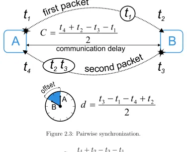
Pair-wise synchronization procedure (also called round-trip synchroniza-tion) is widely used to synchronize two WSN nodes (Fig. 2.3). During his procedure, node A sends a packet with a time-stamp t1 to node B. Upon
the packet reception, node B records its time t2. This value is equal to the
sum of t1, communication delay C and the offset between the clocks of the nodes d:
t2 = t1 +C +d (2.2)
Then node B sends a response packet with a time-stamp t3 to node A.
This second packet contains the value t2 as well. Finally, node A makes a
time-stamp t4 when the second packet is received. If the communication latency is symmetric, i.e. equal in both directions, the value of t4 is given
by:
t4 = t3 +C −d (2.3)
Subtraction of (2.3) from (2.2) allows to find the clock offset d:
t4 −t2 = t3 + C −d−t1 −C −d (2.4)
d = t3 −t1 −t4 +t2
2 (2.5)
Also, the sum of (2.3) and (2.2) can be used to calculate the communication delay C:
A
B
t
1
t
2t
4t
3communication delay A B
2
2 4 13
t
t
t
t
d
=
-
-
+
2
1 3 2
4
t
t
t
t
C
=
+
-
-t
1t
3second pa
cke
t
firs
t pac
ket
t
2Figure 2.3: Pairwise synchronization.
C = t4 +t2 −t3 −t1
2 (2.7)
After the abovementioned message exchange is done, node A has all values necessary to find d and C. As soon as the value of d is known, node A can estimate the time of node B.
2.5.3 Reference broadcasting
A
B
t
ARt
BRRef.
t
BRt
ARd
BA= t
BR- t
ARd
AB= t
AR- t
BRFigure 2.4: Reference broadcasting.
Such uncertainty can be reduced significantly by means of another well known WSN synchronization procedure, often referred to asreceiver-receiver synchronization or reference broadcasting. A group of WSN nodes, which follow this procedure, have to receive one radio message from a special reference node. The receivers record their time values when the reference message arrives, and then each of the receivers broadcasts the correspond-ing time-stamp to all the nodes within its communication range. After reception of such time-stamps, a node A can estimate the offset of its clock with respect to the clock of some other node B as follows:
dAB = tAR −tBR (2.8)
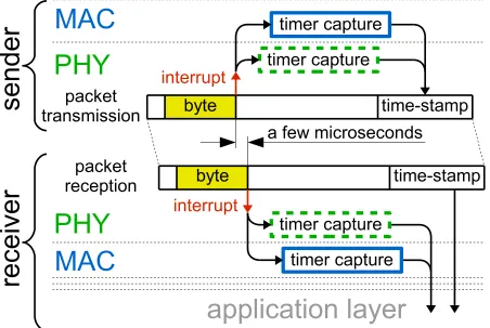
mes-Figure 2.5: Time-stamping of a radio packet at MAC and physical layers.
sage reception takes some time, which changes from node to node. As a consequence, the absolute values of the two relative clock offsets, computed by any pair of receivers, differ.
2.5.4 MAC-layer time-stamping
signal of CC2420 radio [63]). The timer value is recorded by a special interrupt handling routine implemented at the MAC-layer of the sending node. Then the same routine sends the recorded time-stamp to the physical layer, where the time-stamp is attached to the end of the packet, or in-serted somewhere after the aforementioned byte. This happens, of course, after this byte is completely transmitted. A receiver records its local time when the reception of the same byte is completed, which happens only a few microseconds after the byte has been transmitted by the sender. When the whole packet is received, the receiver has a pair of time-stamps, which are taken almost simultaneously on the two nodes. Therefore, the receiver can estimate its clock offset with respect to the sender to a high accuracy simply by subtracting one time-stamp from the other as in (2.1). Thus, many WSN nodes can be accurately synchronized to the reference time if they receive and time-stamp only one radio packet, containing a MAC-layer time-stamp of the node with the reference clock.
2.5.5 Physical layer time-stamping
(dashed rectangles in Fig. 2.5) and can be read by the MCU of a WSN node (e.g. as in Freescale MC13192 transceiver [20]). Physical layer time-stamping is generally more accurate since it does not need interrupt service routines that may cause jitter.
2.5.6 Clock drift estimation
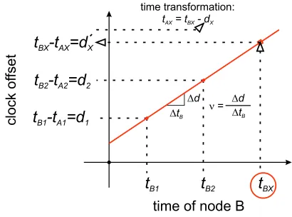
WSN nodes exhibit different clock speeds due to the differences between the frequencies of their crystal oscillators, which results in continuous growth of the absolute values of clock offsets. Therefore, the uncertainty of time synchronization begins to grow immediately after two nodes A and B com-pute their clock offsets. This causes the need to estimate time differences periodically, and the accuracy of the resulting synchronization typically de-pends on how often that estimation is done. More efficient synchronization can be performed under the assumption that the trend of the offset growth is linear. In this case, for example, it is possible to estimate the change of the time offset d = tB −tA per unit of time of node B. This quantity is the relative clock drift rate ν, which can be found using just two values of the clock offset d1 and d2 observed recently at tB1 and tB2 according to the
time of node B:
ν = d2 −d1
tB2 −tB1
= (tB2 −tA2)−(tB1 −tA1)
tB2 −tB1
(2.9)
If ν is known, any time-stamp tBX of node B can be transformed to the corresponding time tAX:
tAX = tBX −dX = tBX −d2 −ν(tBX −tB2) (2.10)
where the offset dX is computed as the sum of the most recently known offsetd2 and the estimated offset change during the respective time interval
tBX−tB2 according to the clock of node B (Fig. 2.6). There is always some
t
B1t
B2t
BXt -t =d
BX AX Xtime transformation:
t = t
-AX BX dX
Dd
Dt
B
n= Dd
Dt
B
clock of
fset
t -t =d
B2 A2 2t -t =d
B1 A1 1time of node B
Figure 2.6: Time-stamp transformation using the relative drift rate.
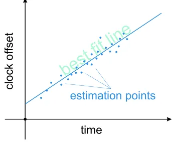
affects the accuracy of the computed relative drift rate. This issue can be addressed by means of linear regression, which is indeed used in recent high-accuracy time synchronization algorithms for WSN [17, 42]. In order to synchronize a WSN node, this technique requires several pairs of time-stamps, which are obtained after the node receives several synchronization messages from a time reference over some time interval. Time stamps are used to compute the corresponding clock offsets, and then the linear regression is performed on this set of values to build a best-fit line (Fig. 2.7). The best-fit line is used to predict offset values in the future, thus keeping the clock of the node synchronized to the reference clock.
be
st
fit
lin
e
estimation points
clock of
fset
time
Figure 2.7: Best-fit line.
In this case it would be sufficient to find the clock drift rate once and then always use it to transform the reading of one clock to that of the other, thus maintaining the common time. However, due to the aging and variable environmental factors, the crystal oscillator frequency changes over time. Therefore, whatever accurate method is used to synchronize WSN nodes, the synchronization procedure must always be repeated after some time.
2.6
Up-to-date methods of WSN synchronization
hard-ware and energy resources available on typical WSN nodes. In order to address such problems, in recent years several WSN-specific synchroniza-tion protocols have been proposed. However, the most known approaches to time synchronization in WSN are focused on achieving the best possible synchronization accuracy (in the order of some microseconds) for the whole network without considering energy saving.
2.6.1 High-accuracy synchronization methods
hop. TSS protocol synchronizes multi-hop networks with highly dynamic topologies at the expense of low overhead. However, the synchronization uncertainty tends to increase unpredictably with the number of hops.
• Reference-broadcast synchronization (RBS) [17] proposed by Elson et al., is based on the procedure described in detail in Subsection 2.5.3: a special reference node sends radio messages to its one-hop neighbors, which time-stamp the messages upon reception, and then exchange the time stamp values. Every node uses these values to compute instanta-neous relative offsets of its clock with respect to the clocks of the other nodes (except the reference node). The nodes also compute their relative clock drift rates by means of least-square linear regression. The knowledge of the relative clock drift rate allows to transform the time of one node to that of another node even in the absence of communication between them during a long term. RBS divides multi-hop networks into one-hop clusters with mutual gateway nodes transforming the time of one cluster to that of another cluster. As experiments showed, RBS synchronized Berkeley Motes within 11 µs. Besides, the protocol operation was verified on the 802.11 network composed of Compaq IPAQs running Familiar Linux: RBS synchronized that network within 6.29 ±6.45 µs, and within 1.85 ±1.28 µs using kernel time-stamping. The synchronization accuracy achieved by RBS is close to the clock resolution. However, the protocol may cause high computation and communication overhead, since all the receivers of the reference message have to exchange their time-stamps and build the cor-responding best-fit lines. The authors of RBS first introduced the concept of receiver-receiver synchronization, which was used later in many other WSN synchronization protocols.
as-signed a level number. The root of the tree has a level 0 and functions as a reference node. At the beginning of the level discovery phase, the root broadcasts a level discovery packet, which contains the root ID and level number. The nodes within the root communication range receive that packet and assign themselves a level number, grater by one than the level number in the received packet. Then those nodes broadcast new level dis-covery packets with their own level numbers. This process continues until all network nodes have their level numbers. In the second, synchroniza-tion phase, the root broadcasts a special packet to initiate synchronization. This packet is received by the immediate neighbors of the root, and then each of the neighbors initiates an exchange of two radio messages with the root after some random time interval. During this exchange, a node sends a message to the root, and the root sends back an acknowledgment. Both messages are time-stamped just before transmission and upon recep-tion, and the time-stamp values are used by the node to compute its clock offset with respect to the root using the procedure described in Subsec-tion 2.5.2. The neighbors of the node overhear its communicaSubsec-tion with the root, and then, after a random time interval, get synchronized to the node in a similar manner, i.e. by means of pair-wise synchronization. This process continues until all network nodes are synchronized. Experiments with Berkeley Motes proved that TPSN synchronizes two adjacent network nodes within 16.9µs. TPSN can synchronize large networks to a high accu-racy. However, the protocol requires the hierarchical network organization, maintaining of which takes much energy, especially when network nodes are mobile.
containing its time-stamps. A network node records its local time upon reception of a synchronization message (using MAC-layer time-stamping), thus obtaining one reference point, which contains two time values: global time and local time. When a node collects a sufficient number of reference points, it computes the drift rate of its clock with respect to the leader clock using linear regression (see subsection 2.5.6). This node can estimate the global time and transmit it to the other nodes which are not yet syn-chronized. The nodes within the leader transmission range receive global time values directly from the leader, the distant nodes receive estimations of the global time from the other synchronized nodes. FTSP operation was experimentally verified on the network composed of 60 Mica2 motes. In 14 minutes, the 6-hop network was completely synchronized to the average accuracy of 3 µs resulting in a 0.5 µs per hop accuracy. FTSP achieves a high synchronization accuracy and it is tolerant to heavy changes of the network topology. However, multiple transmissions of synchronization messages, performed by many nodes, may cause collisions and, as a conse-quence, significant communication overhead.
2.6.2 Light-weight synchronization methods
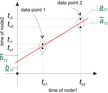
• Tiny-sync and mini-sync (TS/MS) protocols [58], developed by Si-chitiu and Veerarittiphan, form a hierarchy of network nodes where each parent and child can exchange time-stamped radio messages. The oscillator frequencies of network nodes are considered to be approximately constant during time intervals ranging from some minutes to some hours. As a con-sequence, the relationship between clock values t1 and t2 read at the same
time on any two nodes is assumed to be linear:
t1 = a12t2 +b12 (2.11)
where a12 and b12 are the relative drift rate and relative offset of the clocks
of the two nodes, respectively. If node 1 knows the values a12 and b12, it
can estimate the time of node 2 using (2.11). In order to do this, node 1 sends a time-stamped probe message at t0 to node 2. Node 2 receives and timestamps the probe message with its time tb and immediately sends it to node 1 in a response message. Node 1 receives and time-stamps the response message with its time tr (Fig. 2.8). Thus, each message exchange gives to node 1 one data point composed of three values: t0,tb and tr. Since the time-stamp tb was registered after t0 and before tr, the time t0b which
could be observed by node 1 when node 2 registered tb is limited by t0 and
tr. Since t0b could also be computed by (2.11), the following inequalities hold:
t0 < a12tb +b12 (2.12)
tr > a12tb +b12 (2.13)
At least two data points allow to compute lower a12 and upper a12 bounds
of a12 and lower b12 and upper b12 bounds of b12. This can be represented
graphically as two lines with the slopes corresponding to the minimum and maximum values of a12 and the offsets corresponding to the minimum and
Figure 2.8: TS/MS operation: probe message exchange.
as the average values of the aforementioned extreme values (this is rep-resented by the line with the average slope and offset). Node 1 receives several data points, and when a new data point is received, it is compared with the existing ones and one of the data points is discarded. Only the data points providing the best-fit line are kept in the memory. During the probe message exchange, if node 2 does not respond immediately, which will be most likely in real communication, it responds at time tb2 > tb.
This does not affect the correctness of the approach described above, but it just results in two data points: [t0, tb, tr] and [t0, tb2, tr]. Mini-sync
uses more data points to achieve a higher synchronization accuracy at the expense of an increased energy consumption due to a larger number of communication events. Tiny-sync uses minimum number of data points, and saves power at the expense of reduced synchronization accuracy. Two experiments with an 802.11b multi-hop network were used to assess the performance of Tiny-sync. In the first experiment, two computers within one hop exchanged probe messages once per second during 83 minutes, which gave almost 5000 data points. The resulting offset and drift bounds were ±945 µs and ±0.27 ppm, respectively. The second experiment was performed similarly, but two computers were five hops away. This resulted in the offset bound ±3.232 ms and the drift bound ±1.1 ppm. TS/MS al-gorithms provide tight bounds on the relative drifts and offsets of network nodes at the cost of very low computational, memory and communication overhead. However, TS/MS use a hierarchical network organization and therefore is vulnerable to the network topology changes.
pairwise synchronization is performed between parents and children in the tree (see subsection 2.5.2). In the first, centralized algorithm, a reference node, which is the root of the tree, synchronizes with its single hop neigh-bors, then they synchronize with their children etc., until all leaf nodes of the tree are synchronized. The reference node must provide an accurate time, and must resynchronize the network periodically. The resynchroniza-tion period is calculated by the reference node depending on the desired accuracy, upper bound of the clock drift rate and depth of the tree. The upper bound of the clock drift rate in the network is considered to be known in advance. In the second, distributed algorithm, network nodes decide on their own whether they need to be synchronized. A node that requires synchronization sends a request to the closest reference node. If these two nodes are not within a single hop from each other, the request goes along some multi-hop route through intermediate nodes, which get synchronized too. The LTS functionality was verified using Omnet++, a discrete event simulator. In simulations, LTS run during 10 hours on 500 nodes placed in 120×120 m area with the target accuracy of 0.5 s. The average clock offset in the network before synchronization did not exceed 0.4 s, i.e. it was within the accuracy bounds. The centralized LTS scheme is more efficient for the network-wide synchronization, while the distributed scheme better saves power when only a part of network nodes need to be synchronized. LTS requires the construction of a spanning tree, which takes much energy if the network topology changes.
(a) (b) (c)
Figure 2.10: TSync operation: parent node broadcasts announcement message (a); ran-domly chosen node k replies (b); parent node broadcasts synchronization message (c).
channels are used for parent-child communication in the tree: control chan-nel, which is common for all nodes, and clock chanchan-nel, which is unique for each node. At the timet1 against its timescale, the parent node broadcasts
a timestamped announcement message on the control channel to its chil-dren (Fig. 2.10(a)). The announcement message also contains the number
ar-rival, received from node k (Fig. 2.10(c)). Every child node i receives the synchronization message and uses the value t2k to compute the offset of its clock dik with respect to the clock of node k:
dik = t2i−t2k (2.14) Finally, every child i adjusts its clock to the parent time tp:
tp = ti +dik +dk (2.15)
where ti is the current time of a certain nodei. ITR performs synchroniza-tion in the same way as HRTS but on demand of a particular node. The authors of TSync evaluated its accuracy by running it on a WSN composed of five GPS-enabled Nymph nodes with MANTIS operating system. The reported values of mean synchronization error are 21.2 µs for two nodes within one-hop and 29.5 µs for two nodes located tree hops away. TSync performs only three message exchange on each level of the constructed hier-archy, which saves power. Although the usage of dedicated radio channels involves higher implementation complexity, Tsync can be adapted to WSN that use only one channel. However, TSync relies on a hierarchical commu-nication, which makes this service vulnerable to network topology changes.
2.6.3 Adaptive synchronization methods
air. The activated nodes can help to locate the source of pollution more precisely, since they will collect a larger amount of data and at a higher rate. Moreover, the network may need a better time synchronization accuracy in order to compute the velocity and direction of the pollutant diffusion. The described case shows that it is desirable to have time synchronization schemes that combine various specific algorithms and apply them selec-tively depending on the situation. Such flexible techniques should be able to keep track on variable conditions and synchronize the network nodes in the most energy-efficient way. Some adaptive synchronization schemes are emerging, which save energy by keeping the synchronization events as rare as possible while maintaining the desired synchronization accu-racy [49, 6, 56, 21].
• An adaptive time synchronization protocol (authors do not designate it by any name), devised by PalChaudhuri et al. [49], uses the minimum possible number of synchronization messages to achieve a required accu-racy with a certain probability. In this scheme, each of the dedicated network nodes sends time-stamped radio messages to a set of receivers. The receivers register the arrival time of those reference messages, and use linear regression to compute the offset and drift rate of their clocks with respect to the sender clock. Then they send the computed values back to the sender, which uses this information to find its relative clock drift rate and to broadcast it in a special packet to all receivers. After that, any pair of receivers can compute their relative clock drift rates and offsets. Assuming that the distribution of the synchronization errors is Gaussian, the authors prove the following relationship between the probability that a synchronization error is less than the upper boundmax and the minimum number of synchronization messages n:
P (|| ≤ max) = 2erf
√
nmax
σ
where σ is the standard deviation of the distribution. Also, the authors derive an expression for the maximum synchronization error γmax that can develop in the network given the synchronization interval Tsync:
γmax = max+ (Tsync +δmax)νmax (2.17)
whereδmaxis the maximum delay after the synchronization has been started,
νmax is the maximum clock drift rate among the network nodes. The de-scribed adaptive protocol is able to save power due to the probabilistic synchronization, which causes less overhead. However, the protocol may be not suitable for safety-critical applications.
• The energy efficient time synchronization protocol (ETSP), proposed by Shahzad at al. [56], saves energy by minimizing the number of nizations, depending on the number of network nodes requiring synchro-nization. This technique is based on the observation that receiver-receiver synchronization (which is used in RBS) requires less transmissions than sender-receiver synchronization (as in TPSN) when the number of net-work nodes is small. On the contrary, the sender-receiver approach is more energy-efficient in large and dense networks. In ETSP, a parent node synchronizes a group of its children using an RBS-like algorithm, if their number is less or equal to a certain threshold. If the number of children nodes exceeds the threshold, TPSN method is used.
conditions.
2.7
Summary
Time synchronization is essential for the operation of wireless sensor net-works. Most of the well known approaches to time synchronization for WSNs are focused on achieving high synchronization accuracy for the whole network without addressing the power consumption problem. Other solu-tions improve power efficiency by reducing the synchronization complexity, or by enlarging the synchronization period. Recently, also some adaptive synchronization techniques for WSNs have been developed, whose common goal is to save energy by keeping the synchronization events as rare as pos-sible on the basis of the actual synchronization status of the network.
Time Uncertainty in WSN
3.1
Time Estimation Uncertainty
3.1.1 Modeling of Time Estimation Uncertainty
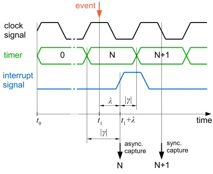
A WSN node measures time with its MCU timer/counter register, which counts cycles of the periodic signal supplied from the crystal resonator (see section 2.2). When some event happens, a special interrupt signal (e.g. a positive pulse on one of the microcontroller pins) can be generated to copy the timer value to the capture register. After the timer value is captured, it can be used by the program running on the MCU. Assume that the timer is reset and starts counting at real time t0. The timer value N is captured after an event happens at real time t1. Thus, if no overflow occurs, the
timer counts N cycles during the real time interval ∆t= t1−t0. The WSN
node can estimate that time interval as following:
∆test =
N f0
(3.1)
where ∆test is the time interval estimate and f0 is the nominal oscillation
frequency of the crystal. However, the actual frequency of the resonator differs from f0, and this difference changes over time due to various
time in terms of an integer number of clock cycles (i.e. time measurement result is discrete), which limits the accuracy of the estimation (3.1). Fi-nally, when an event happens, the timer value is not captured instantly, but after some delay. Taking into account all these factors, the result of 3.1 can be modeled as follows:
∆test = 1
f0
t1+λ+γ Z
t0
f(t)dt (3.2)
where:
• f(t) is the instantaneous frequency of the resonator.
• λ is the random delay between the moment when the event happens and the moment when the corresponding interrupt signal is generated.
• γ is a random error due to the discrete representation of time by the timer value (discretization error).
The component
t1+λ+γ R
t0
f(t)dt models the captured timer value, i.e. exactly
N clock cycles occurs during the real time interval [t0,t1+λ+γ]. Fig. 3.1 illustrates the meaning of λ and γ. Obviously, λ ≥ 0, since the inter-rupt is generated only after the event has happened. The sign and range of γ depends on whether the time capture is done asynchronously to the clock signal or not. Asynchronous capture is done immediately as soon as an interrupt signal arrives. In this case, γ ≤ 0, because the integer number of clock cycles counted by the timer is always equal or less than the real number of cycles at the moment when the interrupt happens, and
t1+λ+γ R
t0
f(t)dt=
$
t1+λ R
t0
f(t)dt
%
, where bc represents the floor function.
Figure 3.1: Time capture.
of a clock cycle (i.e. when the timer value does not change). In this case,
γ ≤0 if the interrupt signal arrives in the first half of the current cycle. In-deed, the integer number of cycles captured on the middle clock edge is still the same as in the first half of the cycle and is less than the corresponding
real number of cycles:
t1+λ+γ R
t0
f(t)dt=
$
t1+λ R
t0
f(t)dt
%
. When the interrupt
happens in the second half of a clock cycle, the synchronous capture is performed in the middle of the next cycle. As a consequence, the captured timer value is more than the real number of cycles at the moment when
the interrupt happens. In this caseγ ≥0 and
t1+λ+γ R
t0
f(t)dt=
&
t1+λ R
t0
f(t)dt
'
where de represents the ceiling function. Thus γ ∈ [−dcycle
2 ,
dcycle
2 ] when the
capture is synchronous.
The uncertainty δ of the time interval estimation (3.1) is:
δ = ∆test −∆t= 1
f0
t1+λ+γ Z
t0
f(t)dt−∆t (3.3)
The instantaneous resonator frequency f(t) can be modeled as:
f(t) =f0 + ∆fman + ∆foper(t) + ∆fage(t) + ∆ff luc(t) (3.4) where:
• ∆fman is a constant frequency deviation due to the imprecision in the angle at which the crystal is cut during its manufacturing process [53];
• ∆foper(t) is a change in frequency caused by operating conditions such as temperature, input voltage, humidity and vibration [31, 70];
• ∆fage(t) is a frequency deviation related to the crystal aging [31, 70];
• ∆ff luc(t) is a frequency deviation due to the random short-term fre-quency fluctuations such as white phase modulation (WPM) noise, flicker phase modulation (FPM) noise, white frequency modulation (WFM) noise, flicker frequency modulation (FFM) noise, and random walk frequency modulation (RWFM) noise [8, 12, 70].
frequency drift [28, 2, 68]. All these terms stand for a difference between the actual and nominal frequencies divided by the nominal frequency. In order to emphasize the relationship between the instantaneous frequency and relative frequency deviation due various factors, the expression (3.4) can be written as
f(t) =f0(1 + ∆
fman
f0
+ ∆foper(t)
f0
+ ∆fage(t)
f0
+ ∆ff luc(t)
f0
) (3.5)
or as
f(t) =f0(1 +yman +yoper(t) +yage(t) +yf luc(t)) (3.6) whereyman = ∆ffman0 is the normalized frequency deviation due to the crystal manufacturing process and yoper(t) = ∆
foper(t)
f0 , yage(t) =
∆fage(t)
f0 , yf luc(t) =
∆ff luc(t)
f0 are instantaneous normalized frequency deviations due to operating
conditions, crystal aging and random short-term frequency fluctuations respectively.
The frequency stability can be approximately considered as a sum of maximum values ofyman,yoper(t),yage(t) andyf luc(t). However, commercial manufacturers often assume a crystal operation life of only a few years, thus ignoring aging during a longer term [31]. Military specifications generally indicate the frequency stability related to the operation in an extended temperature range and the impact of factors such as humidity, shock and vibrations.
The constant frequency drift yman of commercial quartz crystals can be in the order of 20-50 ppm [53]. The major part of yoper(t) is the drift in the order of 10-20 ppm caused by the temperature. The temperature-dependent frequency driftytemp is not linear with temperature. For AT-cut crystals ytemp can be approximated as
ytemp(T) ≈ K1(T −T0)3 +K2(T −T0) +K3 (3.7)
where T is temperature and K1, K2, K3, T0 are unique to each
fre-quency deviation versus temperature and the shape of that curve does not change with time, i.e. ytemp is constant if the temperature is stable [31]. The frequency drift caused by the crystal aging yage(t) changes with time, and new crystals age faster than old ones (e.g. 5 ppm in the first year of operation, and then 3 ppm [31]). In stable environmental conditions, aging typically exhibits logarithmic dependence on time [68, 71, 70, 47, 9, 48]:
yage(t) = A1log(1 +A2t) (3.8)
where coefficients A1 and A2 are usually determined from the least square
fit using the measurement results. However, after an initial stabilization period (usually 30 days) the aging is often considered as approximately linear function of time and is specified in ppm/year [29, 71]. The effect of random frequency fluctuations is generally estimated by means of the Allan variance over a certain time interval [8, 70]. The order of magnitude of the corresponding standard deviation estimated over 1 s is some nanoseconds for low cost XO [70, 2].
The rough estimate of the drift magnitudes given above allows to say that during a medium-term of operation the frequency deviation is mainly caused by the crystal cut imprecision and deviation of temperature from the standard ambient temperature (+25◦C ±3◦C). In this case, the resonator frequency approximates to:
f = f0(1 +ys) (3.9)
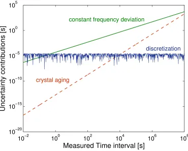
10−2 100 102 104 106 108 10−20
10−15 10−10 10−5 100 105
Measured Time interval [s]
Uncertainty contributions [s]
constant frequency deviation
discretization
crystal aging
Figure 3.2: Individual contributions of time measurement uncertainty due to the constant deviation of the oscillator frequency (solid line), crystal aging (dashed line) and time discretization (noisy pattern). All terms are plotted as a function of the measured time intervals on a logarithmic scale.
gives an approximate expression for the time estimation uncertainty:
δ ≈ 1 f0
t1 Z
t0
f0(1 +ys)dt−∆t (3.10) Taking into account that ys is constant and ∆t = t1 − t0, (3.10) can be
simplified as:
δ ≈ys∆t (3.11)
drift change due to aging is 2.5 ppm/year and f0=32.768 kHz. These values are in accordance with the features of the XOs commonly used on com-mercial WSN nodes, such as the TelosB/Tmote Sky modules. In Fig. 3.2 individual uncertainty contributions due to the discretization (noisy pat-tern), constant frequency offset (solid line) and crystal aging (dashed line) are shown on a logarithmic scale as a function of increasingly large mea-sured time intervals. Notice that for very short time intervals (i.e. below 1 s) the discretization is the main source of uncertainty, whereas the aging effect becomes significant only after about 3 years. In all the intermediate cases, the measurement uncertainty is dominated by the frequency offset. Since the typical operational lifetime of a WSN node is in the order of some weeks, and the periodic synchronization operations are not repeated very frequently in order to save power, the expression (3.11) can be used to model the overall time estimation uncertainty in most of the situations of practical interest.
3.1.2 Clock Drifts Measurements
Figure 3.3: Experimental setup used to measure the clock drifts of WSN nodes with respect to a stable reference signal produced by a function generator Agilent 33220A.
(Fig. 3.3). The nodes were programmed to record their timer values at each rising edge of the reference signal. The ambient temperature was stable during the whole experiment (around +22◦C) performed in a lab-oratory. In Fig. 3.4 the differences between the values measured by the MCU timers of the nodes are plotted against the reference values provided by the function generator. Notice that these differences exhibit essentially a linear trend with a slope that is constant for a given node. This means that during the experiment the total frequency deviation was dominated by the constant frequency deviation ys of the employed resonator, while all the other contributions were negligible. Therefore, the time estimation uncertainty is indeed a linear function of the measured time interval under stable environmental conditions, as expected, and the approximate expres-sion (3.11) holds in most of practical cases.
10 20 30 40 50 60 0
20 40 60 80 100 120
Clock offset [ms]
Elapsed time [minutes]
Figure 3.4: Measured offsets between the clocks of 10 TelosB and Tmote Sky nodes and the time values provided by a function generator Agilent 33220A. The nodes measure time once per minute by reading their 32-bit timers clocked at 32.768 kHz.
0 10 20 30 40 50 60 70 80 90 −20
0 20 40 60 80 100 120
Elapsed time [min]
Clock offset [ms]
heating
node 1
node 2
Figure 3.5: Measured offsets between the clocks of 4 TelosB modules and time values provided by a function generator Agilent 33220A. The nodes measure time once per minute by reading their 32-bit timers clocked at 32.768 kHz.
two dashed lines), while the clock drift rate of the other two nodes remains constant. Clearly, the resonator frequency of node 2 is more sensitive to the temperature, and the clock drift rate of node 2 even changes its sign during heating.
In Fig. 3.6(a) and Fig. 3.6(b) the clock offsets of the heated nodes with respect to reference time values and the air temperature measured by the nodes are plotted against the time values provided by the function gen-erator. Although clock offsets exhibit a linear trend with time when the temperature is approximately constant (around +22◦C during the first 30
obvi-0 10 20 30 40 50 60 70
Elapsed time [min]
Clock offset [ms]
temperature measured by node 1
clock offset of node 1
0 10 20 30 40 50 60 70 80 9020
25 30 35 40 45 50 Temperature [ ° C] (a) 0 5 10 15 20 25 30
Elapsed time [min]
Clock offset [ms]
temperature measured by node 2
clock offset of node 2
0 10 20 30 40 50 60 70 80 9020
25 30 35 40 45 50 Temperature [ ° C] (b)
ous, especially in Fig. 3.6(b) during the last 30 minutes of experiment, when node 2 gradually cools down. The results of this experiment emphasize the impact of temperature on the accuracy of time estimation performed by WSN nodes.
3.2
Time Transfer Uncertainty
When transferring a certain time value between two WSN nodes, the time of the sender will be actually available at the receiver end only after some delay. Such a latency depends on the amount of operations occurring between the moment when the sender timer is read and the instant in which the receiver time is updated. As known, in case of an end-to-end, single-hop transmission the total latency includes the following terms [34]:
• send time, namely the nondeterministic time spent by a transmitter for building the packet at the application layer and for transferring the packet to the MAC layer. This time depends on the interaction between the MCU and the RF module, on the processor load as well as on the OS scheduling algorithms;
• access time, i.e. the random, MAC-specific time spent to access the wireless channel. Such a delay depends on the network traffic as well as on the features of the communication protocol;
• transmission time, i.e. the time to turn an equivalent bit of informa-tion into modulated electromagnetic waves just before transmission;
• propagation time taken by one bit to cross the wireless channel from the sender to the receiver;
• receive time including both the time to transfer the packet from the MAC layer to the application layer and the time to process the packet, e.g. to extract the received time value.
If a carrier sense multiple access with collision avoidance (CSMA/CA) protocol is used, the overall end-to-end latency δC can be modeled by a random variable resulting from the addition of three major terms, i.e.:
δC = δS +δL +δR (3.12)
where:
• δS and δR coincide with the send time and the receive time, respec-tively;
• δL is the link and physical layer latency which includes one or mul-tiple values of access, transmission, propagation and reception time depending on the number of retransmission attempts in case of busy channel or packet collision.
In order to have a clearer insight about the features of the three individual terms mentioned above, several δS, δL and δR values were measured using an automatic experimental setup based on an oscilloscope controlled by a PC. In particular, after identifying (from the documentation of the TelosB module [45] and radio transceiver CC2420 [63]) which pins of the radio chip can be used to generate pulses at the beginning and at the end of δS,
δL and δR intervals during a packet transmission, we used the oscilloscope to measure the time differences between the pulse edges delimiting the various latency contributions. Notice that this approach leads to very accurate results, because software-related delays almost do not affect the measurement process.
Figure 3.7: Experimental setup to measure communication delays.
3.2.1 Experimental Setup and Measurement Procedure
The basic components of the proposed experimental setup are shown in Fig. 3.7 and include not only one sender and receiver, but also a random traffic generator, namely a node that is explicitly used to emulate a known amount of traffic within the network, as it will be explained in the next subsections. All measurements were performed on TelosB nodes running TinyOS [26]. Each TelosB node is equipped with an IEEE 802.15.4 com-pliant 2.4 GHz radio transceiver CC2420 [63], which is controlled by a microcontroller MSP430F1611 [64] via Serial Peripheral Interface (SPI).
(a) (b)
Figure 3.8: Flowcharts of the applications running on the sender (a) and receiver (b).
The flowcharts of the applications running on the sender and receiver nodes are shown in Figures 3.8(a) and 3.8(b).
Figure 3.9: Test signals used to measure different components of the communication delay. Signal edges correspond to the boundaries between different stages of radio packet transmission and reception.
reception are shown in Fig. 3.9. The long segmented rectangle on the top of Fig. 3.9 represents the transmission of the radio packet by the sender, the bottom rectangle (identical to the upper one, but shifted to the right) represents the reception of the same radio packet by the receiver.
In the experiments the pins of either MCU or radio chip of the trans-mitting and receiving nodes were connected to the channels of a digital storage oscilloscope (DSO) TDS 3012 [62]. A LabVIEW application con-trolled the oscilloscope through an Ethernet interface. The application was specifically designed for measuring the time interval between the voltage pulses acquired on the two channels, with a pulse edge on the first channel set as a triggering event. Eventually, multiple measured time values were saved in a log file in order to be analyzed later.
Figure 3.10: Two test pulses measured during the transmission of a radio packet with a payload of 40 bytes.
pulses is 12.50 ms and corresponds to the total communication delay. Con-sider that the instrumental uncertainty associated to such a measurement result is negligible, because the worst-case contributions affecting the time measurements using the chosen oscilloscope are several order of magnitude smaller than the interval under test. In fact, the delay time accuracy of the oscilloscope is ±200 ppm over any time interval longer than 1 ms [62]. Also, according to the MSP430F1611 manual [65], moving a constant to a certain destination address requires 5 CPU cycles. Therefore, since the microcontroller operates at the frequency of 8 MHz, the commands setting or clearing a port pin should take less than 1 µs.
3.2.2 Send and Receive Time
20 40 60 80 100 0
1 2 3 4 5 6 7 8
Payload size [Bytes]
δS [ms]
Figure 3.11: Average send time values (solid central line) and±σ limits (dashed lines) as a function of the payload size. The mean and standard deviation values used to plot the picture are estimated using sets of 100 measurement results for different payload sizes.
between two nodes. The average values (solid central line) and the ±σ
limits (dashed lines) of the estimated send time are shown in Fig. 3.11 as a function of the payload size. Notice that delay is random but it grows linearly with packet size. This is reasonable because if the MCU transfers the packet to the radio module through a serial connection (SPI), the send time depends on the packet length. As a consequence, the send time can be modeled as
δS = tS(D +H) + S (3.13)
where:
• D is the payload size (e.g. expressed in bytes);
• H is the fixed number of additional overhead bytes (i.e. H=10 bytes in TinyOS 2.0);
the average time to transfer 1 byte over the serial connection;
• S is a random variable including all the other possible random
con-tributions such as the latency of the interrupt service routine reading the timer or the time spent by the MCU in running other tasks.
In general, it is not possible to provide a unique stochastic description of
S due to the excessive number of factors affecting this term. However,
according to the performed experiments, S exhibits approximately a
uni-form distribution with mean value equal to 3.4 ms and standard deviation of about 1.4 ms. This contribution is most probably dominated by the random delay introduced o