Visualization and exploratory analysis of epidemiologic data using a novel space time information system

(1)

Open Access

Research

Visualization and exploratory analysis of epidemiologic data using a

novel space time information system

Gillian A AvRuskin*

1

_{, Geoffrey M Jacquez}

1

_{, Jaymie R Meliker}

2

_,

Melissa J Slotnick

2

_{, Andrew M Kaufmann}

1

_{and Jerome O Nriagu}

2

Address: 1_{BioMedware Inc., 516 N. State St., Ann Arbor, MI 48104, USA and}2_{Department of Environmental Health Sciences, School of Public}

Health, University of Michigan, Ann Arbor, MI 48109–2029, USA

Email: Gillian A AvRuskin* - [email protected]; Geoffrey M Jacquez - [email protected];

Jaymie R Meliker - [email protected]; Melissa J Slotnick - [email protected]; Andrew M Kaufmann - [email protected]; Jerome O Nriagu - [email protected]

* Corresponding author

Abstract

Background: Recent years have seen an expansion in the use of Geographic Information Systems (GIS) in environmental health research. In this field GIS can be used to detect disease clustering, to analyze access to hospital emergency care, to predict environmental outbreaks, and to estimate exposure to toxic compounds. Despite these advances the inability of GIS to properly handle temporal information is increasingly recognised as a significant constraint. The effective representation and visualization of both spatial and temporal dimensions therefore is expected to significantly enhance our ability to undertake environmental health research using time-referenced geospatial data. Especially for diseases with long latency periods (such as cancer) the ability to represent, quantify and model individual exposure through time is a critical component of risk estimation. In response to this need a STIS – a Space Time Information System has been developed to visualize and analyze objects simultaneously through space and time.

Results: In this paper we present a "first use" of a STIS in a case-control study of the relationship between arsenic exposure and bladder cancer in south eastern Michigan. Individual arsenic exposure is reconstructed by incorporating spatiotemporal data including residential mobility and drinking water habits. The unique contribution of the STIS is its ability to visualize and analyze residential histories over different temporal scales. Participant information is viewed and statistically analyzed using dynamic views in which values of an attribute change through time. These views include tables, graphs (such as histograms and scatterplots), and maps. In addition, these views can be linked and synchronized for complex data exploration using cartographic brushing, statistical brushing, and animation.

Conclusion: The STIS provides new and powerful ways to visualize and analyze how individual exposure and associated environmental variables change through time. We expect to see innovative space-time methods being utilized in future environmental health research now that the successful "first use" of a STIS in exposure reconstruction has been accomplished.

Published: 08 November 2004

International Journal of Health Geographics 2004, 3:26 doi:10.1186/1476-072X-3-26

Received: 09 September 2004 Accepted: 08 November 2004

(2)

Background

Geographic Information Systems are beneficial tools in modelling static representations of reality; however they fall short in their ability to handle time. The ability to store, visualize, and analyze both the temporal and spatial dimension of data continues to be a challenging task. Over the past decade, there have been several attempts to include time enabled capabilities into GIS. [1] and [2] proposed amendment vectors to extend the vector data model to the time dimension, while others enhanced the grid data model to represent snap-shots of raster data at different time intervals [3]. Although temporal extensions exist, e.g. [2] commercial GIS packages do not properly support tem-poral aspects of spatial data [4].

The importance of GIS for medical research and epidemiol-ogy has long been recognized [5-7], and GIS is frequently used for retrospective exposure reconstruction [8-10]. However the application of GIS to risk and exposure assess-ment has historically focused on the hazard as the object of interest – such as the locations of contaminated industrial sites with high concentrations of carcinogens – instead of the individual [3]. More recently exposure assessment using GIS has targeted individuals in their present homes, but relatively little attention has been placed on individual exposure reconstruction involving residential histories and past activities. This in large part is due to the poor ability of current GISs to handle multitemporal geographic informa-tion and the movement of individuals within the context of putative exposure sources whose locations and output change through time. Consequently, there have been few attempts to expand on the 'static map' to provide a more accurate view of exposure.

The ability to effectively represent, query, and model the temporal dimension is expected to significantly enhance researchers' abilities to undertake environmental health research with georeferenced data. Studying an individual's exposure over time is a key factor in determining risk, par-ticularly for diseases with long latency periods such as cancer [3], because individual exposure to environmental contaminants (eg carcinogens) can change as people move through space over time. Exposure assessment char-acterizes the concentration of potential toxins, as well as the frequency and duration of contacts between individu-als and those toxins. Therefore, accurate exposure assess-ment requires estimation of variation in contaminant concentration as well as changes in geographic proximity to contaminant sources over time. This requires models that can account for residential histories and how residen-tial location influences ambient contaminant concentra-tions as well as exposure opportunities.

In this research we applied a STIS to visualize and analyze data from a bladder cancer case-control study. The objective

of the epidemiologic research project is to identify a range of factors that have contributed to bladder cancer incidence in Michigan, with the focus on spatial and spatiotemporal patterns of exposure to naturally occurring arsenic in drink-ing water. Cases are recruited from the Michigan State Can-cer Registry and diagnosed in the years 2000–2003. Controls are frequency matched to cases by age (± 5 years), race, and gender, and recruited using a random digit dialing procedure from an age-weighted list. To be eligible for inclusion in the study, participants must have lived in the eleven county study area for at least the past five years and had no prior history of cancer (with the exception of non-melanoma skin cancer). The goal is to enroll 1400 partici-pants in total. This is an ongoing five year project and only some preliminary spatiotemporal datasets, visualization tools, and results are shown here. Conclusive results will not be available for a few more years, until data has been collected and analyzed for all 1400 participants. The STIS is being developed at BioMedware, in Ann Arbor Michigan with funding from the National Institutes of Environmen-tal Health Sciences and the National Cancer Institute. In this paper STIS is used to visualize and analyze data from a bladder cancer case-control study but it can also be used for health/environment interactions or marketplace sales trends. More information about the STIS and a free 30 day download can be evaluated at http://www.terraseer.com/ products/stis.html.

Results and discussion

Data from a case-control study of bladder cancer in south eastern Michigan was used to evaluate the efficacy of the STIS for documenting and visualizing space-time relationships between cases, controls and putative risk factors. Lifetime exposure to arsenic in drinking water (an element that has been associated with bladder cancer at high levels [12,13]) was reconstructed for each individual by incorporating spati-otemporal information about residential mobility (every address inhabited since birth), occupational history (every full time job since the age of 16), drinking water patterns, and concentration of arsenic in drinking water.

Space time information system

(3)

Within the space time coordinate, in addition to the well known descriptors (e.g. latitude, longitude), we also spec-ify a movement model that defines how the object moves through space as a function of time. Among the simplest of movement models is an instantaneous displacement such that the object ceases to exist at one location and immediately reappears at another location. We use this simple model to describe residential histories.

Morphing describes how the shape of geographic features (such as lines and polygons) changes through time. Here an object is comprised of multiple vertices changing shape through time by the addition, deletion and movement of vertices. This is called network morphing (for lines) and polygon morphing (for polygons). Morphing can be grad-ual, in which case the change in the object's shape occurs over a defined time interval; or it can be abrupt. In our research we utilize this approach to model cadastral sys-tems and the realignment of administrative and political boundaries. This allows us to track, for example, how municipal water districts change through time, and to then estimate arsenic exposure from drinking water for individuals on municipal water supplies.

Attributes are observations on variables describing the modelled entity and its environment (e.g. case/control identifier, population size, ethnicity, etc.) Our data model assumes observations occur at discrete times at which the attributes of an object are quantified. Attribute change models describe how the values of attributes change between observation times. The simplest attribute change model is a step function that updates an attribute's value when a new observation is made on that attribute. More complex change functions that obtain values from nearby

locations are used to interpolate values through space and time for both categorical and continuous data [14]. These include techniques from the field of geostatistics that pro-vide a probabilistic framework for space-time interpola-tion by building on the joint spatial and temporal dependence between observations [15]. In this research we use the step function approach to model, for example, change in arsenic concentration in potable water when an individual's water supply source is switched from one source of supply to another. We also use geostatistics to model how arsenic concentration in ground water changes spatially and as a function of geology (described in [16]).

Study data

We reconstructed individual exposures by incorporating spatiotemporal data on residential mobility (where people have lived throughout their lives), water supplies (private well, city well water, or city surface water), and drinking water habits. Only locations in which the participants have lived or worked for longer than one year were collected and geocoded. Data about diet, smoking, and medical history were also collected by a phone interview or written ques-tionnaire. A point file (where each point represents a partic-ipant) was then imported into the STIS along with associated database files containing attribute information such as address and primary source of drinking water. Table 1 is an example of the drinking water and residential mobil-ity database. Even though information for only three partic-ipants is shown, seven different addresses and nine different sources of drinking water are represented. (Street addresses are not shown to protect participant's identity). Therefore, a change in address or primary source of water warrants a new row in the database.

Table 1: Part of database of participant addresses and water source information Information for four participants is shown. For each change in address or primary source of water a new row is entered in the database. Therefore there are 16 rows in this sample database.

Year moved in Year moved out Sample ID City Primary Source of Water

9/12/1935 1/1/1953 1 Swartz Creek Private well 1/1/1956 1/1/1958 1 Swartz Creek Private well, softener 1/1/1958 1/1/1963 1 Swartz Creek Private well 1/1/1963 1/1/1974 1 Swartz Creek Private well, reverse osmosis 1/1/1974 1/1/1990 1 Swartz Creek new private well 1/1/1990 1/1/2002 1 Swartz Creek Community Supply 1/1/2002 1/1/2004 1 Swartz Creek Community Supply, softener 1/1/1976 1/1/1990 2 Livonia Community Supply

1/1/1990 1/1/2004 2 Brighton CS (township well and treatment plant) 1/1/1953 1/1/1961 3 Jackson Community Supply

(4)

Other point files were imported including present and historical data on industries and contaminated sites in the study area. A township map and water supply boundary map were imported as polygons. In addition to temporal changes in attributes such as township population, source of community's water supply, and number of people served, town boundaries and water supply boundaries changed with time. New towns were incorporated, com-munity systems expanded their borders, and occasionally, communities were combined and town boundaries dis-solved. All of these temporal changes were handled using attribute change models and morphing.

Importing spatiotemporal datasets

We imported shapefiles describing the above data using the STIS data import facility that allows the variables to be time stamped. The user is prompted to import vector information into a new geography or an existing geogra-phy (if new information is to be added to an already exist-ing geographic layer the latter will be chosen). The user must tell the system whether the data is (1) a time slice

(similar to a collection of GIS static maps) where changes take place at specified times for all objects in the dataset, or (2) a time series where data varies asynchronously and objects move or change attributes at different times. For example Census data are time slice data – attributes remain constant for a decade (1980–1990) and then all attributes are updated with the next decade's census infor-mation (1990–2000). On the other hand, data associated with tracking residential histories are time series data, with household moves occurring at different times for each individual. The system imports data at temporal granularities varying from seconds to years; and the data may then be analyzed at these different time scales.

Visualization procedures

Being able to visualize changes in boundaries and attribute values over time is an effective approach to better understanding and exploring data. Because time is a dimension of the data rather than an attribute all views of the data are easily animated. Analogous to a static GIS, attributes of data are visualized by specifying colour, shape, and size of graphical elements (e.g. symbols). However, in contrast to a GIS, the STIS easily facilitates visualization of changing polygon shapes and attribute values over time by animating maps, histograms, and tables simultaneously. Valuable information that might be lost in an atemporal GIS is captured and can become the focus of analysis in the STIS. There are four major vis-ualization views – maps, graphs (histograms, scatter plots, box plots), tables, and time plots.

(1) The map view displays spatial data and the user inter-acts with the maps by zooming, panning, selecting, and querying. The added feature of the STIS is the animation

toolbar. It is employed to show individuals changing place of residence through time; arsenic-emitting indus-tries being founded, operating, and going out of business; municipal water supply districts growing and coalescing; and attribute values, such as arsenic concentrations, changing through time.

(2) In the STIS histograms, scatter plots, and box plots are also animated over time. An individual or group of individuals (e.g. cases vs. controls) may be selected at one point in time and the user can explore how that selection's values change through time. For example, we used this feature to explore how individual arsenic exposure changed over a participant's lifetime. We also used it to compare esti-mated arsenic burdens for the cases to those of the control population.

(3) Table views also are animated, as the given value of a variable (such as the arsenic concentration in a municipal water supply) will change through time. Tables thus show how data values change over time by updating a given objects value when it increases or decreases.

(4) The time plot graphs time on the x-axis and the value of a variable, such as estimated arsenic exposure, on the y-axis. Objects of interest, such as cases and controls, then map into this bivariate time plot to explore time depend-encies in arsenic exposure. Unlike the other views, the time plot is not animated because it already shows the entire time range of the data on the x-axis.

A novel feature of the STIS is the ability to time-link visual-ization windows. Maps, statistical graphics, and tables may be time-linked so that all of the views are synchro-nized to the same point in time. Animating the time-linked windows then displays the views simultaneously changing through time. We use this feature to display the changing residential locations of the cases and controls along with the locations and emission volumes of arsenic-producing industries. All of this is done within the context of municipal water districts whose boundaries morph and whose arsenic concentrations are dynamic. While this map visualization is occurring we observe how the fre-quency distributions of modelled arsenic exposure are changing for the cases relative to that of the controls. Par-ticipants (cases or controls) are thus easily evaluated and compared to other participants in terms of their residen-tial histories, and population-level characteristics, such as the mean and dispersion for arsenic exposure estimates, may be compared statistically as they evolve over time.

(5)

participant ID's of the cases and controls, or the names of the municipal water districts) to link together correspond-ing values on the maps and statistical graphics. Statistical brushing is used to select objects (such as the points on a scatter plot) and to then highlight the corresponding objects on maps and other statistical graphics.

Carto-graphic brushing occurs when objects are selected on a map, and their corresponding values on the statistical graphics are highlighted. We used statistical brushing to select participants with high arsenic exposures, and to then identify their locations on maps of their residential histories. We use cartographic brushing to explore

possi-Change in water supply systems over 50 years (1935, 1965, 1995) Figure 1

Change in water supply systems over 50 years (1935, 1965, 1995) Over the years many towns in Oakland County and Genesee County begin to purchase surface water (from Detroit).

Participant movement over 20 years Figure 2

(6)

ble associations between proximity to arsenic emitting industries and the local densities of cases relative to the controls.

Application of visualization procedures

We first investigate changes in the water supply systems (Figure 1). It is clear that over a 50 year interval (from 1935–1995) private well owners and some community ground water systems replaced their private wells or ground water systems with a purchased surface water sys-tem (hooking up to a larger syssys-tem such as the Detroit Sewer and Water System). Visualizing this information over time is valuable as it shows areas that historically might have been associated with high arsenic levels. It also is used to help assign arsenic concentrations to previ-ous residences. For some public ground or surface water

systems historic arsenic concentrations have been recorded. For participants on such water supply systems we therefore can directly assign water source arsenic con-centrations. Historic arsenic concentrations for well water supplies often are not available, and for these we interpo-late arsenic concentration values using geostatistical pro-cedures that account for values in nearby wells, spatial covariance in these values, and their dependency on pre-dictors such as groundwater geology [16].

Visualizing the movement of bladder cancer cases and controls through time is crucial in our analysis of arsenic exposure and how it relates to the incidence of bladder cancer. Figure 2 presents participants at three different time points (1960, 1982, 2001). A case is represented by a circle and a control by a square. In 1960 there were two

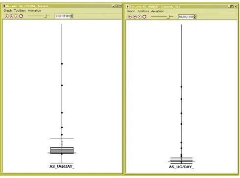
Box plot of arsenic exposure in 1988 for cases (left) and controls (right) Figure 3

(7)

cases and one control. By 1982 four more cases and two more controls moved into the study area and in 2001 the same number of cases and controls remain in the area. Note that one case and one control have moved resi-dences. The animated map thus informs us regarding the residential mobility of the cases and controls. Spatial and temporal subsets of these populations can then be selected and statistically analyzed and summarized using other visualization windows and statistical methods.

Analysis of arsenic exposure

In this analysis we are interested in the temporal variabil-ity in arsenic exposure in cases versus controls as well as clusters of high arsenic values. Arsenic exposure was calcu-lated by multiplying arsenic concentration (µg/L) by home consumption of water and beverages made with water (L/day) at each residence and for each change in water consumption. Data regarding water and beverage consumption was obtained via survey [17]. We utilize the box plot to look at means and interquartile ranges through time (Figure 3 for 1988). The windows are time linked and show cases (on the left) and controls (on the right). A more evenly distributed exposure to arsenic in the case subset is indicated by the large interquartile, and 1.5X interquartile range.

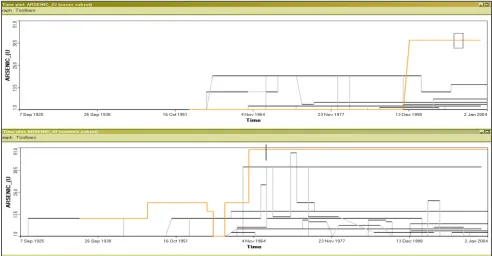
Time graph of arsenic exposure in cases (top) and controls (bottom) Figure 4

Time graph of arsenic exposure in cases (top) and controls (bottom) Notice the increase in arsenic for both sets after 1951. The increase in arsenic is much larger for controls and remains high for at least two individuals.

Arsenic in drinking water (2003/2004) Figure 5

(8)

The time plot is another visualization method and pro-vides information over the entire time range (Figure 4 x-axis equals time, y-x-axis represents arsenic exposure). This graph shows general trends in this preliminary dataset. In the early 1960's arsenic exposure was actually greater for controls (bottom graph) than for cases (upper graph). We also notice that the highest arsenic value (51 µg/L) occurred for a control in 1964 and lasted until the end of the study period. The highest value for a case (38 µg/L) occurred later in the study period (1990). All records are linked to the map view and an investigation of geograph-ical clustering can occur in tandem with the temporal analysis of the time plot.

In addition to the graphical analysis we employed statisti-cal clustering methods to identify spatial clusters of homes with high arsenic concentrations in their water supplies. The Univariate Local Moran is a statistical method used to detect local spatial autocorrelation by

decomposing Moran's I into contributions for each loca-tion. Here, each location refers to an arsenic value sam-pled at the home of each participant. Moran's I is a weighted correlation coefficient that is used to determine whether neighbouring areas are more similar than would be expected under the null hypothesis. In this study the local Moran statistic is used to detect where there are statistically significant clusters of high (or low) arsenic values in participants' drinking water. Data regarding arsenic in drinking water was collected at the kitchen tap of each participant from their present residence. Water samples were stored on ice, acidified with 0.2% trace metal grade nitric acid, and refrigerated until analysis. Water samples were subsequently analyzed for arsenic using an inductively coupled plasma mass spectrometer (ICP-MS, Argilent Technologies Model 7500 c) [17]. A map of arsenic values from participants' drinking water is shown in Figure 5. The Local Moran analysis was per-formed on this arsenic dataset resulting in a map of

signif-Local Moran analysis at two spatial scales Figure 6

(9)

icant clusters (identifying areas as high-high clusters, low-low clusters, low-low-high outliers, high-low-low outliers, and areas not significant from background), and a local moran scatterplot. Figure 6 is the result of the local Moran analy-sis using spatial weights of five (left) and ten (right) near-est neighbours, with 999 randomizations, at the alpha level of 0.05. Generally the two maps look similar, and this is corroborated by similar Global Moran's I values of 0.126279 for five nearest neighbours and 0.129596 for ten nearest neighbours. However, there are differences that arise from analysing spatial pattern at two different local spatial scales. For example, in the northern region of the ten nearest neighbour map we find high-high values indicating high arsenic values surrounded by other high arsenic values. We also see an area of low-low values in the western part of the map, around Lansing. Households in these low-low locations are generally on community water supplies where arsenic values are kept below 50 µg/ L to comply with Environmental Protection Agency stand-ards. Conducting the Local Moran analysis at different neighbourhood sizes allows one to evaluate the sensitivity of clustering to different spatial scales.

Conclusions

In this paper we presented a novel application of a space time information system to analyze some preliminary data in an ongoing case-control bladder cancer study. This approach is significant in that it not only visualizes the movement and attribute changes of spatial objects (including cases, controls, arsenic producing industries, and municipal water supplies) but also allows the user to compare values of these objects over time by time-linking windows. This ability to handle high temporal resolution data is enabling new approaches to exposure assessment. In the near future the STIS will be able to integrate expo-sure assessment models using an Application Program-mers Interface (API). Users will have the flexibility to program specific models outside the software and then visualize their outcome in the STIS using the API. For less technically sophisticated users, a methods toolbar will be included, where common modelling algorithms will be made available using a simple calculator-type interface. Other plans for the software include importing and sup-porting raster files, exsup-porting animated maps as movies (for presentations), visualizing geospatial lifelines [18,19] in a separate window once objects are selected, and adding spatiotemporal clustering statistics to the methods toolbar.

Competing interests

Some authors are also affiliated with BioMedware a research company that also develops software for the exploratory spatial and temporal analysis of health and environmental data. With funding from the National

Cancer Institute, GMJ, AMK, and GAA developed STIS, which is a commercial product of Terraseer.

Acknowledgements

Development of the STIS software was funded by grants R43 ES10220 from the National Institutes of Environmental Health Sciences and R01 CA92669 from the National Cancer Institute. The epidemiologic component was supported by grant R01 CA96002-10, Geographic-Based Research in Can-cer Control and Epidemiology, from the National CanCan-cer Institute.

References

1. Hazelton NWJ: Integrating time, dynamic modeling and GIS: Development of four-dimensional GIS. In PhD thesis The Uni-versity of Melbourne, Department of Surveying and Land Information; 1991.

2. Langran G: Time in Geographic Information Systems London: Taylor and Francis; 1992.

3. Mark D PI, Bian L, Rogerson P, Vena J, Egenhofer M PI: "Spatio-Temporal GIS analysis for environmental health,".National Institute of Environmental Health Sciences, National Institutes of Health . R01 ES09816-01

4. Camossi E, Bertolotto M, Bertino E, Guerrini G: A Multigranular spatiotemporal data model. In Proceedings of the Eleventh ACM International Symposium on Advances in Geographic Information Systems: New Orleans, Louisiana, USA . November 7–8, 2003

5. Barnes S, Peck A: Mapping the future of health care: GIS appli-cations in health care analysis. Geographic Information Systems

1994, 4:31-33.

6. Clarke KC, McLafferty SL, Tempalski BJ: On epidemiology and geographic information systems: A review and discussion of future directions.Emerging Infectious Diseases 1996, 2:85-92. 7. Croner CM, Sperling J, Broome FR: Geographic Information

Sys-tems (GIS): New perspectives in understanding human health and environmental relationships.Statistics in Medicine

1996, 15:1961-1977.

8. Ward MH, Nuckols JR, Weigel SJ, Maxwell SK, Cantor KP, Miller RS:

Identifying populations potentially exposed to agricultural pesticides using remote sensing and a geographic informa-tion system.Environmental Health Perspectives 2000, 108:5-12. 9. Bellander T, Berglind N, Gustavsson P, Jonson T, Nyberg F, Pershagen

G, Jarup L: Using geographic information systems to assess individual historical exposure to air pollution from traffic and house heating in Stockholm. Environmental Health Perspectives

2001, 109:633-639.

10. Elgethun K, Fenske RA, Yost MG, Palcisko GJ: Time-location anal-ysis for exposure assessment studies of children using a novel global positioning system instrument. Environmental Health Perspectives 2003, 111:115-122.

11. Bates MN, Smith AH, Cantor KP: Case-control study of bladder cancer and arsenic in drinking water. American Journal of Epidemiology 1995, 141:523-530.

12. Chen CJ, Chuang YC, You SL, Lin TM, Wu HY: A retrospective study on malignant neoplasms of bladder, lung and liver in blackfoot disease endemic area in Taiwan. British Journal of Cancer 1997, 53:399-405.

13. Smith AH, Goycolea M, Haque R, Biggs ML: Marked increase in bladder and lung cancer mortality in a region of northern Chile due to arsenic in drinking water. American Journal of Epidemiology 1998, 147:660-669.

14. Jacquez GM, Greiling DA, Kaufmann AM: Design and implemen-tation of space-time information systems.Journal of Geographi-cal Systems in press.

15. Kyriakidis PC, Journel AG: Geostatistical space-time models: a review.Mathematical Geology 1999, 31:651-684.

16. Goovaerts P, Avruskin G, Meliker J, Slotnick M, Jacquez G, Nriagu J:

Modelling uncertainty about pollutant concentration and human exposure using geostatistics and a space-time infor-mation system: Application to arsenic in groundwater of Southeast Michigan. In Accuracy 2004: Proceedings of the 6th Inter-national Symposium on Spatial Accuracy Assessment in Natural Resources and Environmental Sciences, Portland 2004.

(10)

Publish with BioMed Central and every scientist can read your work free of charge "BioMed Central will be the most significant development for disseminating the results of biomedical researc h in our lifetime."

Sir Paul Nurse, Cancer Research UK

Your research papers will be:

available free of charge to the entire biomedical community

peer reviewed and published immediately upon acceptance

cited in PubMed and archived on PubMed Central

yours — you keep the copyright

Submit your manuscript here:

http://www.biomedcentral.com/info/publishing_adv.asp

BioMedcentral epidemiology: Application of spatio-temporal visualization

tools.Journal of Geographical Systems in press.

18. Hornsby K, Egenhofer M: Modelling moving objects over multi-ple granularities.Special issue on Spatial and Temporal Granularity, Annals of Mathematics and Artificial Intelligence 2002, 36:177-194. 19. Miller H: What about people in geographic information