R E S E A R C H A R T I C L E
Open Access
Feasibility of retrieving dust properties and
total column water vapor from solar
spectra measured using a lander camera
on Mars
Naohiro Manago
1*, Katsuyuki Noguchi
2, George L. Hashimoto
3, Hiroki Senshu
4, Naohito Otobe
5,
Makoto Suzuki
6and Hiroaki Kuze
1Abstract
Dust and water vapor are important constituents in the Martian atmosphere, exerting significant influence on the heat balance of the atmosphere and surface. We have developed a method to retrieve optical and physical properties of Martian dust from spectral intensities of direct and scattered solar radiation to be measured using a multi-wavelength environmental camera onboard a Mars lander. Martian dust is assumed to be composed of silicate-like substrate and hematite-like inclusion, having spheroidal shape with a monomodal gamma size distribution. Error analysis based on simulated data reveals that appropriate combinations of three bands centered at 450, 550, and 675 nm wavelengths and 4 scattering angles of 3°, 10°, 50°, and 120° lead to good retrieval of four dust parameters, namely, aerosol optical depth, effective radius and variance of size distribution, and volume mixing ratio of hematite. Retrieval error increases when some of the observational parameters such as color ratio or aureole are omitted from the retrieval. Also, the capability of retrieving total column water vapor is examined through observations of direct and scattered solar radiation intensities at 925, 935, and 972 nm. The simulation and error analysis presented here will be useful for designing an environmental camera that can elucidate the dust and water vapor properties in a future Mars lander mission.
Keywords:Mars atmosphere, Dust particles, Total column water vapor, Direct solar radiation, Scattered solar radiation, Radiative transfer simulation, Inverse analysis
Introduction
Dust floating in the Martian atmosphere plays an im-portant role in determining the circulation of atmos-phere, since dust is an important heat source in the atmosphere due to the absorption of solar radiation (Gierasch and Goody 1972; Moriyama 1975; Smith 2008). Accurate knowledge of the temporal and spatial distribution of dust particles, as well as their optical pa-rameters, is indispensable for understanding their impact on the heat balance of the planet. Also, it is known that a trace amount of water vapor exists in the Martian at-mosphere (Fedorova et al. 2009; Smith 2009; Smith, et
al. 2009; Whiteway et al. 2009). The condensation of water vapor leads to the formation of water ice clouds, which can also affect the heat balance of the Martian at-mosphere (Flasar and Goody 1976; Haberle et al. 2001; Hinson and Wilson 2004).
Observations of air-borne dust and water vapor in the Martian atmosphere have been performed by Mars or-biters and landers as well as ground-based observations (Smith 2008). As compared with orbiter observations, lander measurements are less likely to be influenced by changes in surface albedo. The dust source is on the sur-face of Mars, and the concentration of dust is highest near the surface. Thus, compared with orbiters, more ac-curate measurement can be done from landers. Also, local parameters such as pressure and temperature can be measured precisely from landers. Among the various * Correspondence:[email protected]
1Center for Environmental Remote Sensing, Chiba University, 1-33 Yayoi-cho,
Inage-ku, Chiba-shi, Chiba 263-8522, Japan
Full list of author information is available at the end of the article
observational methods used so far, the measurements of direct solar radiation (DSR) and scattered solar radiation (SSR) with cameras onboard Mars landers have brought a wealth of information on dust properties. The optical depth of dust can be retrieved as a function of wave-length from DSR measurement, while other optical properties and information on the composition of dust particles can be extracted by coupled analysis of DSR and SSR intensities.
The first observation of dust in the Martian atmos-phere was made with the Imaging Camera (Patterson et al. 1977) onboard the Viking Lander (Pollack et al. 1977, 1979, 1995). The optical depth of dust was measured with the Imager for Mars Pathfinder (IMP) experiment (Smith et al. 1997), which revealed seasonal variation similar to the result of the Viking observation, with lim-ited inter-annual variations (Smith and Lemmon 1999; Tomasko et al. 1999; Markiewicz et al. 1999). Subse-quently, similar observations were made with Panchro-matic Cameras (Pancam, onboard the Spirit and Opportunity rovers) (Bell et al. 2003; Bell et al. 2004a, 2004b; Lemmon et al. 2004), a Surface Stereo Imager (SSI) (onboard the Phoenix) (Lemmon et al. 2008; Moores et al. 2010), and Mastcam (onboard Curiosity) (Malin et al. 2010; Moore et al. 2016). The first observa-tion of water vapor in the Martian atmosphere was car-ried out with the IMP (Titov et al. 1999), in which 6 spectral bands around 940 nm were employed.
The effective radius (reff) and its variance (veff) are the
most important parameters that determine dust’s optical behavior. As reviewed by Tomasko et al. (1999), the most plausible values forreffandvefffrom early
observa-tions are in a range of 1.2–1.8μm and 0.2–1.0, respect-ively. In subsequent missions such as Spirit and Opportunity, the value of reff was estimated to be
~1.5 μm (with the value of veff fixed at 0.2). The lidar
observation of Phoenix reported values between 1.2 and 1.4 μm (Komguem et al. 2013). The variation in thereff
estimated by several missions may indicate that there are temporal and spatial variations of dust properties. Thus, it is desirable to carry out long-term observations at various locations on the Mars surface to monitor changes in dust properties.
The most dominant composition of Martian dust is considered to be basalt, and its weathering products due presumably to past volcanic activity (Dabrowska et al. 2015). The reflectance spectrum in the wavelength range of 0.3–2.5 μm suggests that the rock type is most likely palagonites, the partially recrystallized products of basalt-glass influenced by wind erosion (Dlugach et al. 2003). The value of the real part of the refractive index (RI) is ~1.5 at a wavelength of 0.5 μm, which is close to the value of silicate. The imaginary part, on the other hand, is negligibly small in visible and near-infrared
wavelengths, but its value substantially increases toward the shorter wavelengths, suggesting the contribution of iron oxide components (Dlugach et al. 2003). Thus, it is possible that dust particles contain small amounts of crystalline ferric materials such as goethite, hematite, and/or maghemite.
In this paper, we examine the feasibility of retrieving dust properties and total column water vapor (TCWV) in the Martian atmosphere with a camera system on-board a lander. Such camera observation can be realized by modifying a lander camera system with the addition of optical filters. We develop a dust model in which dust properties are parameterized with a small number of
“dust model parameters”, including optical depth, effect-ive radius/variance of dust size distribution, volume mix-ing ratio of hematite, complex RI of silicate, and scale height of dust. Since Martian dust’s properties are sim-pler than those of terrestrial aerosols, we can safely as-sume a simple dust model. A relatively small number (seven) of dust model parameters are used in this model, which helps to alleviate the underconstrained (ill-posed) nature of the inverse problem. These parameter values are optimized by fitting a small number of “ observa-tional parameters” based on DSR and SSR measure-ments. Only three wavelength bands are utilized for dust observations, which helps keep camera hardware size and data transmission requirements small. Another set of two or three wavelengths around 935 nm is postu-lated for extracting TCWV from DSR/SSR measure-ments. We also examine the feasibility of such a camera measurement on the basis of sensor specifications cur-rently available.
Methods/Experimental
Dust model based on non-spherical shape and monomodal size distribution
First, we describe the model used to parameterize the optical and physical properties of Martian dust. Basically, the present model is relevant to the physical conditions of dust particles including their composition, shape, and spatial distribution in the Martian atmosphere. The dust composition can be parameterized with a complex RI that depends on substance and wavelength,λ. From past studies (e.g., Hamilton and Christensen 2005 and refer-ences therein), it is plausible that Martian dust is mostly composed of silicates, with small amounts of iron oxides such as hematite. Thus, in the present analysis, we as-sume a two-component dust model with silicate sub-strate and hematite inclusion. Similar treatment of a multi-component aerosol was employed in the analysis of the terrestrial atmosphere (Manago and Kuze 2010; Manago et al. 2011). The complex RI value of silicate (n0=m0−k0i,i: imaginary unit) can be characterized with
visible light (e.g., Table 1 in Dabrowska et al. 2015, Table 5 in Levoni et al. 1997), while that of hematite is pa-rameterized as nA(λ) =m(λ)−k(λ)i, in which we should consider the large absorbance of blue light. Referring to Querry (1985) for the wavelength dependence of m (λ) and k (λ), the RI of their mixture, n, can be calculated using Maxwell-Garnett theory (Ehlers et al. 2014) as
n2 ¼n20
n2Aþ2n20þ2ρA n2A−n20
n2
Aþ2n20−ρA n2A−n20
: ð1Þ
Here, ρA is the volume mixing ratio of hematite. Fig-ure 1 shows the wavelength dependence of dust RI re-ported in Wolff et al. (2009). Figure 1 also shows an example of the fitting we did using Eq. (1), resulting in n0= 1.48−0.000942i (m0= 1.48 and k0= 0.000942) for
the complex RI of silicate andρA= 1.77% for the volume mixing ratio of hematite. The agreement between the fit-ting curves and literature curves is satisfactory when considering the small sensitivity of radiance values tom0
and k0, and the derived values ofm0and k0are
consist-ent with reported values for silicate. The advantage of our dust model is that it can reproduce the important features of measured data in spite of the simplicity of the model, being based on just three parameters,m0,k0,
and ρA. We have assumed internal mixing in Fig. 1 as the Maxwell-Garnett theory is applicable to dust parti-cles having internal mixing. Although we tested another model assuming external mixing of silicate and hematite particles, the result exhibited much poorer agreement as compared with internal mixing treatment illustrated in Fig. 1.
Dust particles in the Martian atmosphere can possibly have various shapes, but limited information from direct observations (e.g., Pike et al. 2011) makes it difficult to theoretically formulate their shapes precisely. Moreover, it is difficult to reproduce the effects of non-spherical shapes in a radiative transfer simulation for the Martian atmosphere. To cope with these difficulties, here we propose the use of equivalent volume spheroids with random rotation axes as employed by Dubovik et al.
(2006) to estimate the influence of particle shapes for feldspar samples collected from terrestrial soil. Similarly, here we fix the aspect ratio distribution in such a way that the distribution is zero at aspect ratios less than 1.44, and gradually increases in the aspect ratio range between 1.44 and 3. A detailed discussion on the non-spherical shape effect will be given later. In general, when Maxwell-Garnett theory is applied to spheroids, the resulting RIs exhibit dependence on polarization. Such polarization dependence disappears only for the special case of spherical particles. Nevertheless, we as-sume the polarization-independent form of Eq. (1) for simplicity, though the light scattering calculations are implemented assuming non-spherical dust shapes.
In this research, we assume that the dust size distribu-tion can be expressed with a monomodal gamma distri-bution including only coarse mode particles (Hansen and Travis 1974; Tomasko et al 1999). This assumption is based on the fact that for the optical properties of des-ert dust on the Earth, submicron (fine mode) particles can be ignored, and the size distribution can be treated as virtually monomodal, since most of particles are supermicron and in coarse mode (Dubovik et al. 2006). For completeness, the sensitivity of our model to the ex-istence of fine mode particles will be discussed later. A monomodal gamma distribution can be expressed as
dN
d lnr¼ rξ reffveff
ð ÞξΓð Þξ exp − r reffveff
; ð2Þ
with
ξ¼ 1
veff−2: ð3Þ
Here, r is the particle radius and Nis the number of particles. The gamma function (Γ) is used to normalize
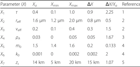
Table 1Dust model parameters (X1–X7)
Parameter (X) Xa Xmin Xmax ΔX ΔX/Xα Reference
X1 τ 0.4 0.1 1.0 0.9 2.25 1
X2 reff 1.6μm 1.2μm 2.0μm 0.8μm 0.5 2
X3 veff 0.2 0.1 0.4 0.3 1.5 2
X4 ρA 0.03 0 0.05 0.05 1.67 3
X5 m0 1.5 1.4 1.6 0.2 0.133 4
X6 k0 0.001 0 0.002 0.002 2 4
X7 zs 14 km 5 km 20 km 15 km 1.07 5
References (1) Smith and Lemmon1999; (2) Tomasko et al.1999; (3) Ehlers et al.2014; (4) Dabrowska et al.2015; (5) Hoekzema et al.2010.
the integral of Eq. (2). Parametersreff andveff are the
ef-fective radius and efef-fective variance, respectively, and they are defined as
reff¼
Z∞
−∞ r3 dN
d lnrd lnr=
Z∞
−∞ r2 dN
d lnrd lnr
" #
ð4Þ
and
veff¼
Z∞
−∞
r2ðr−reffÞ2 dN
d lnrd lnr= r 2 eff
Z∞
−∞ r2 dN
d lnrd lnr
" #
:
ð5Þ
Since our observation is made optically, the most rele-vant parameter is the dust extinction coefficient (αe), which is governed by the size distribution and extinction cross-section of dust particles. We consider the extinc-tion value at wavelength 550 nm, the peak wavelength of solar radiation. It is assumed that αe is homogeneous horizontally, and it decreases exponentially with increas-ing altitude,z:
αeð Þ ¼z τ
zs
exp −z
zs
: ð6Þ
Here,τis the dust optical depth at wavelength 550 nm and zs is the scale height. The typical scale height of aerosols on the Earth is ~2 km. On the other hand, the scale height of Martian dust is typically 10–15 km (Thomas et al. 1999), which is similar to the scale height of pressure (Hoekzema et al. 2010), since the lower at-mosphere is well-mixed on Mars. Besides, the variation range of optical depth of Martian dust is larger than that of terrestrial aerosols: namely, on Mars, typical values of τ are 0.2 (non-dimensional) for relatively clear periods, 1–2 for hot southern summers, and 4–5 during major dust storms (Savijärvi 2014).
In summary, our dust model can be described with only seven parameters: real (m0) and imaginary (k0) parts
of RI of silicate substrate, volume mixing ratio of hematite inclusion (ρA), effective radius (reff) and
effect-ive variance (veff) of size distribution, and optical depth
(τ) and scale height (zs) of extinction coefficient at wave-length 550 nm. Hereafter, these model parameters will be collectively denoted asX. Table 1 lists“a priori” (i.e., the most plausible value before observation, Xa), mini-mum values (Xmin), maximum values (Xmax), and
vari-ation ranges (ΔX=Xmax−Xmin) of the seven parameters
utilized in the present model. When evaluating the im-pact of changes to dust model parameters, it is desirable that the parameters be normalized beforehand so that their variabilities will be on the same scale. Here, we use dust model parameters divided by the variation range (ΔX) listed in Table 1. These normalized dust model
parameters will be collectively denoted asx. The 7th col-umn of Table 1 shows the ratio between ΔX and Xa, which will be used in our later analysis.
Radiative transfer simulation of Martian atmosphere
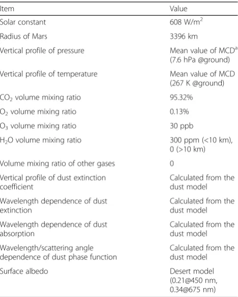
In this research, a radiative transfer simulation code, MODTRAN5 (Berk et al. 2006) is employed to calculate the theoretical spectra of DSR and SSR that would be observed by a Mars lander. Although MODTRAN is a simulation code originally developed for the terrestrial atmosphere, it is applicable to Martian atmosphere by changing parameters such as distance from the Sun and the concentrations of gas components. The main param-eters to be configured for Mars are listed in Table 2. The atmosphere between 0 and 100 km is divided into 36 layers of stratified spherical atmosphere, with the as-sumption of horizontal uniformity. The use of the DIS-ORT algorithm (Stamnes et al. 1988) is desirable for the detailed analysis of SSR in the observation data. In the present simulation study, however, we use Isaacs’ two stream algorithm (Isaacs et al. 1987), which is much fas-ter and the resulting differences in SSR values are esti-mated to be less than 20% (Isaacs et al. 1987). The single scattering algorithm includes spherical geometry of ray transmission, while multiple scattering contributions are calculated using plane parallel geometry (the solar
Table 2Main parameters of MODTRAN to be configured for Martian atmosphere
Item Value
Solar constant 608 W/m2
Radius of Mars 3396 km
Vertical profile of pressure Mean value of MCDa
(7.6 hPa @ground)
Vertical profile of temperature Mean value of MCD (267 K @ground)
CO2volume mixing ratio 95.32%
O2volume mixing ratio 0.13%
O3volume mixing ratio 30 ppb
H2O volume mixing ratio 300 ppm (<10 km),
0 (>10 km)
Volume mixing ratio of other gases 0
Vertical profile of dust extinction coefficient
Calculated from the dust model
Wavelength dependence of dust extinction
Calculated from the dust model
Wavelength dependence of dust absorption
Calculated from the dust model
Wavelength/scattering angle dependence of dust phase function
Calculated from the dust model
Surface albedo Desert model
(0.21@450 nm, 0.34@675 nm)
a
illumination impinging upon each atmospheric level is determined with spherical refractive geometry). The ex-tinction/absorption coefficients and phase function are calculated from the dust model by using a Fortran pro-gram developed by Dubovik et al. (2006); this software calculates optical parameters of spheroidal aerosols by using a look-up table prepared by coupling the T-matrix (Mishchenko and Travis 1998) and approximate geometric-optics integral-equation (Yang and Liou 1996) methods.
Observational parameters for dust retrieval
Spectral irradiance/radiance of DSR/SSR in the visible and near infrared spectral regions is to be measured with an environmental monitor camera onboard a Mars lander. Radiance values of SSR are measured at particu-lar scattering angles (χ); the angle between the original solar ray (hitting the scattering particle) and the line of sight (LOS) from the particle to the observer). Here χ= 0 corresponds to scattering in the forward direction. The expressions DSR(λ) and SSR(λ, χ) can be used to expli-citly specify wavelength or scattering angle. To reduce the total volume of data that must be transmitted during the Mars observation mission, it is vitally important to minimize the number of quantities to be measured (i.e., the number of wavelengths and scattering angles) when designing an observation strategy.
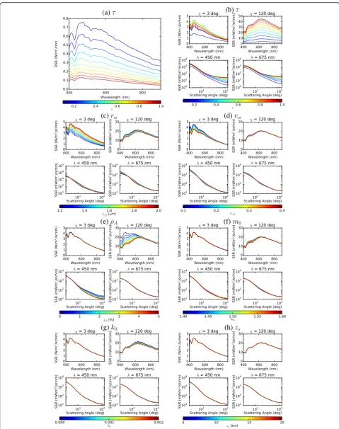
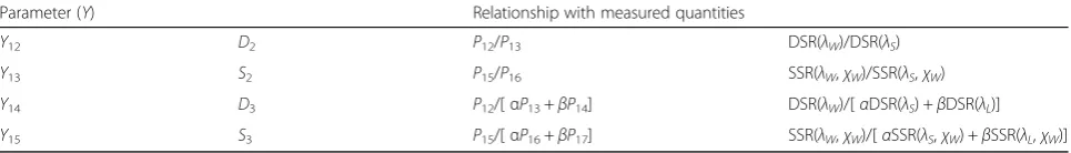
Figure 2 summarizes the results of MODTRAN simu-lation, showing how the values of DSR/SSR depend on wavelength and scattering angle for various values of dust parameters (τ,reff,veff,ρA,m0,k0, andzs). In Fig. 2a,
b, DSR/SSR values are plotted for dust optical depths (τ) between 0.1 and 1. At all wavelengths between 400 and 900 nm, decrease in DSR and increase in SSR are ob-served with increasing τ. Among the seven dust model parameters, DSR shows almost no dependence on pa-rameters other than τ, whereas SSR changes with τ, reff,
veff,ρA,m0, and k0(Fig. 2b–g). Figure 2c shows that the
SSR intensity of forward scattering (χ= 3°) increases at all wavelengths with increasing reff, while Fig. 2d shows
that the forward scattering intensity decreases over the absorption band of hematite (blue range around 450 nm) with increasingveff.
Moreover, Fig. 2e, f shows that the SSR intensity of backward scattering (χ= 120°) decreases over the hematite absorption band with increasing ρA and in-creasingm0, while Fig. 2g shows that the backward
scat-tering intensity decreases at all wavelengths with increasing k0. This is due to the fact that absorption is
stronger at larger scattering angles due to longer effect-ive path length. As seen from Fig. 2h, SSR is hardly af-fected by zs, the dust scale height in the Martian atmosphere.
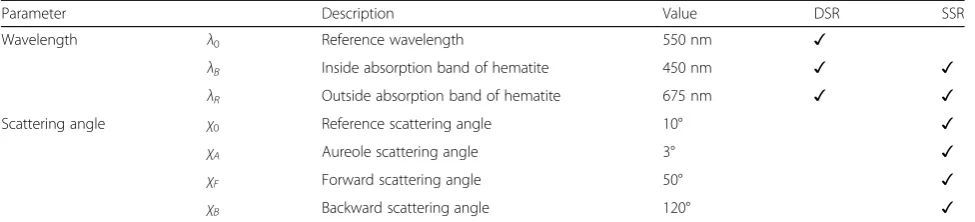
Thus, in order to derive all the necessary dust infor-mation while minimizing redundancy, we selected the wavelengths and scattering angles listed in Table 3. The wavelength band width is chosen to be 10 nm. The mea-surements of DSR spectra are made at the three wave-lengths of (λ0, λB, λR) = (550, 450, 675) (in nm), while SSR spectra are measured at the two wavelengths of (λB, λR) for the four scattering angles (χ0,χA,χF,χB) = (10°, 3°, 50°, 120°). As a result, 11 values are measured as listed in Table 4. The reason for the choices of λB= 450 nm within the hematite absorption band and λR= 675 nm outside the band is that these wavelengths are close to the peak wavelength of SSR radiance (~550 nm) with reasonable sensitivity of a silicon sensor. As shown in Fig. 3, the measurement of SSR is carried out on the almucantar plane (θlos=θsun), where LOS zenith angle
(θlos) is the same as the solar zenith angle (θsun). When
χ> 2θsun, on the other hand, SSR is measured on the
principal plane (θlos=χ−θsun, ϕlos=ϕsun+ 180°), where
LOS azimuth angle (ϕlos) is on the opposite side of the
solar azimuth direction (ϕsun).
So far, we have considered how to choose the min-imal set of quantities to be measured that satisfies the necessary and sufficient conditions for estimating the dust model parameters. Additionally, we have to avoid the influence of measurement error as far as possible. For this purpose, the use of relative values of spectral irradiance/radiance, instead of their abso-lute values, is advantageous for improving the accur-acy of the resulting dust parameters, since precise calibration of a lander camera is difficult and the relative values are less sensitive to calibration errors than absolute values. Therefore, in this research, we calculated the appropriate ratios among the 11 mea-sured quantities listed in Table 4, and we propose the final observational parameter set as listed in Table 5. In the second column of this table, the capital letters, D, A, F, and B indicate direct solar radiation, aureole (i.e., scattered solar radiation in close vicinity to the Sun), forward scattering, and backward scattering, re-spectively, and the subscripts 0, C, B, and R indicate values at the reference wavelength (550 nm), color ra-tio (i.e., intensity rara-tio of blue to red), values at the blue wavelength (450 nm), and values at the red wavelength (675 nm), respectively.
Fig. 2Sensitivity of (a) DSR and (b–h) SSR to dust model parameters. DSR and SSR intensities for various values of dust model parameters (a:τ,b:τ,c:
quantities will be denoted in lower-case letters as p, and observational parameters calculated with the nor-malized measured quantities will be denoted as y.
Observational parameters for water vapor retrieval
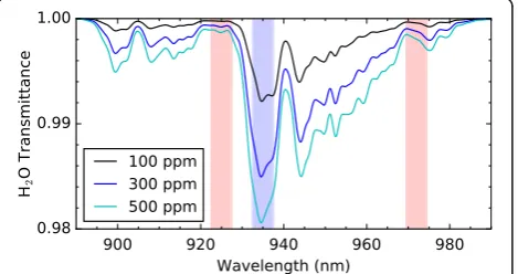
Water vapor absorption bands are located inside the sensitive range (350–1000 nm) of conventional com-plementary metal-oxide semiconductor (CMOS) sen-sors to be employed for our environmental monitor camera. By measuring the absorbance in DSR or SSR spectra, we can measure TCWV (cw) through the Martian atmosphere, where the water vapor concen-tration is very limited (~300 ppm). Among the near-infrared absorption bands, it would be reasonable to employ the strongest absorption band around 930– 970 nm. Here, we assume the atmospheric model pa-rameters listed in Table 2, and we calculate the value of cw by assuming that the volume mixing ratio (VMR) of water vapor is constant below 10 km. The a priori value of cw is 1.43 mg/cm2 for a water vapor VMR of 300 ppm. Figure 4 shows transmittance spec-tra simulated at a solar zenith angle (SZA) of 80° while changing the water vapor VMR as 100, 300, and 500 ppm.
In this study, we calculate values of cw from the ra-tio of DSR or SSR at wavelengths inside and outside the water vapor absorption band. Here, we consider the wavelengths and the scattering angles listed in Table 6. The wavelength band width is chosen to be 5 nm. Since the effective optical path length is larger
at larger scattering angles, the line-of-sight directions of θlos= 85° and ϕlos=ϕsun+ 180° have been chosen
for the SSR measurements.
The measured quantities (P12−P17) are listed in
Table 7, and they are appropriately combined to de-fine the observational parameters as listed in Table 8. When only two wavelengths are available, the outside wavelength should be chosen to be λS= 925 nm,
Table 3Wavelengths and scattering angles chosen for dust observation
Parameter Description Value DSR SSR
Wavelength λ0 Reference wavelength 550 nm ✓
λB Inside absorption band of hematite 450 nm ✓ ✓
λR Outside absorption band of hematite 675 nm ✓ ✓
Scattering angle χ0 Reference scattering angle 10° ✓
χA Aureole scattering angle 3° ✓
χF Forward scattering angle 50° ✓
χB Backward scattering angle 120° ✓
Table 4Measured quantities (P1–P11) of DSR and SSR for dust retrieval
Parameter (P) Measured quantity Parameter (P) Measured quantity
P1 DSR(λ0) P7 SSR(λB,χB)
P2 DSR(λB) P8 SSR(λR,χ0)
P3 DSR(λR) P9 SSR(λR,χA)
P4 SSR(λB,χ0) P10 SSR(λR,χF)
P5 SSR(λB,χA) P11 SSR(λR,χB)
P6 SSR(λB,χF)
which is closer to λW= 935 nm. Then, cw is optimized by matching the calculated ratio of D2= DSR(λW)/ DSR(λS) or similar ratio of SSR (S2) to the measured
one. Alternatively, when three wavelengths are avail-able, non-absorptive wavelengths are chosen at wave-lengths shorter (λS= 925 nm) and longer (λL= 972 nm) than the absorption band. By linear interpolation, a reference intensity at λW (DSR0(λW) = [(λL−λW)DSR(λS) + (λW−λS)DSR(λL)]/(λL−λS) and similar value for SSR) can be obtained that is free of water vapor absorption. Then, cw is found by match-ing the calculated ratio D3= DSR(λW)/DSR0(λW) or a similar one for SSR (S3) to the measured ratio. Using
three wavelengths, more precise estimation of water vapor absorption is possible with better knowledge of the spectral intensity covering the entire range around the absorption band.
Retrieval of model parameters
We consider the optimization of model parameters (in-cluding both dust model parameters and TCWV) through a least squares analysis. We assume a form of
y¼FðxÞ þεy; ð7Þ
where x and yare vectors composed of the normalized values of model parameters and observational parame-ters, respectively,F(x) is a forward model function, and
εyis measurement noise. The Taylor series expansion of
Eq. (7) around the a priori value xa leads to the linear
approximation given as
y¼FðxaÞ þKxðx−xaÞ þεy: ð8Þ
Here,Kx=∂(x)/∂x is the Jacobian matrix. If we ignore measurement noise, Eq. (8) can be solved using a pseudo-inverse matrix of Kx. In reality, however, meas-urement noise is not negligibly small. In order to avoid the instability of the solution due to a lack of sufficient information from the observation, we consider the fol-lowing cost function that includes the residuals of both the observational and model parameters:
cð Þ ¼x ðy−F xð ÞÞTS−y1ðy−F xð ÞÞ
þðx−xaÞTS−1
a ðx−xaÞ: ð9Þ
Here, Sy and Sa are the variance-covariance matrices of the observational parameters and a priori of the model parameters, respectively. The (i, j) element of Sy is the covariance of yi and yj, which is 〈(yi−〈yi〉)(yj−
〈yj〉)〉 , where 〈yi〉 stands for the expectation value of yi (1≤i≤11, see Table 5 for the case of dust retrieval). The i-th diagonal element ofSyrepresents the variance of yi, i.e. 〈(yi−〈yi〉)2〉. Similarly, the off-diagonal and diagonal elements of Sa represent the covariance and variance of a priori, respectively. We optimize the model parameters by minimizing the cost function with iterative calcula-tion based on the non-linear least square method (Rodgers, 2000).
Linear approximation for error estimation
In the following discussion on the retrieval error, for simplicity, we use a linear approximation (the Jacobian is calculated with the a priori). The expectation value (re-trieved solution, xr) of the model parameters can be given as
xr¼xaþ KT
xS−y1KxþS−a1
−1
KT
xS−y1ðy−F xað ÞÞ:
ð10Þ
Here, we have assumed that the errors of observational and model parameters follow Gaussian distributions.
Table 5Observational parameters (Y1–Y11) used for dust retrieval
Parameter (Y) Relationship with measured quantities
Y1 D0 P1 DSR(λ0)
Y2 DC P2/P3 DSR(λB)/DSR(λR)
Y3 AC P5/P9 SSR(λB,χA)/SSR(λR,χA)
Y4 AB P5/P4 SSR(λB,χA)/SSR(λB,χ0)
Y5 AR P9/P8 SSR(λR,χA)/SSR(λR,χ0)
Y6 FC P6/P10 SSR(λB,χF)/SSR(λR,χF)
Y7 FB P6/P4 SSR(λB,χF)/SSR(λB,χ0)
Y8 FR P10/P8 SSR(λR,χF)/SSR(λR,χ0)
Y9 BC P7/P11 SSR(λB,χB)/SSR(λR,χB)
Y10 BB P7/P4 SSR(λB,χB)/SSR(λB,χ0)
Y11 BR P11/P8 SSR(λR,χB)/SSR(λR,χ0)
Fig. 4Transmittance of water vapor in the Martian atmosphere. Values are simulated with a wavelength resolution of 2 nm (FWHM) for volume concentrations of 100, 300, and 500 ppm. Theblue band
Defining a gain matrix asGy=∂xr/∂y= (KTxSy–1Kx+Sa–1)–1 KxTSy–1, we can rewrite Eq. (10) as
xr¼xaþGyðy−F xað ÞÞ: ð11Þ
Furthermore, usingA=∂xr/∂y=GyKx= (KxTSy–1Kx+Sa–1)–1 KTxSy–1KxandGa=∂xr/∂xa= (In−A) = (KxTSy–1Kx+Sa–1)–1 Sa–1, we can rewrite Eq. (11) as
xr¼AxþGaxa: ð12Þ
In Eq. (12), the right-hand side can be regarded as a weighted mean of the model parameter obtained from the true state (x) and the a priori (xa), with weights of KxTSy–1KxandSa–1, respectively. Here,Ais a matrix called the averaging kernel matrix (AKM), its diagonal ele-ments indicating the extent to which the true model pa-rameters affect the retrieved solution.
Adjustment of regularization strength
The weight of the a priori is determined by the balance betweenSyand Sa. From a statistical point of view, the optimum value of Sa would be the actual variance-covariance matrix of a priori (Se). However, it is difficult to estimateSeaccurately. In some cases, better solutions can be obtained by using Sa that are different from Se and adjusting the strength of regularization (i.e., con-straint from the a priori data). Here, we introduce a regularization parameterγas
Sa−1¼γS−1
e : ð13Þ
The regularization strength is increased by increasing the value ofγ. When we increase the regularization par-ameter, at some point the weight on the a priori be-comes non-negligible and the retrieved parameter tends to be drawn toward its a priori value. This results in a gradual increase in the residuals of the observational pa-rameters, since in general, a priori values are different from true values. In accordance with Tikhonov
regularization (Doicu et al. 2010), a good regularization strength is achieved by making it stronger within the range in which the residuals of observational parameters, i.e., the first term of the cost function (9), are almost constant.
Error estimation of model parameters
First, we consider the errors in the retrieved model pa-rameters propagated from both measured values and a priori values. A variance-covariance matrix of the model parameters due to propagation error of measurement (Sm) can be calculated as
Sm¼GySyGT
y: ð14Þ
Similarly, a variance-covariance matrix of model pa-rameters due to a priori error (Ss) can be obtained using Ga=In−Aas
Ss¼GaSeGT
a: ð15Þ
The combined variance-covariance matrix of model parameters including both measurement error and a priori error is given as
Sc¼SmþSs: ð16Þ
The equation Sc= (KxTSy–1Kx+Sa–1)–1holds when γ= 1. If we define error ratioεras
εr¼ diag SsS−c1
1=2
¼diagGaγðAþGaγÞ−11=2; ð17Þ
then we haveεr= [diag(Ga)]1/2whenγ= 1. Each element
ofεr changes from 0 to 1 whenγ changes from 0 to ∞.
In addition to the propagation errors described above, imperfectness of the forward model can cause systematic errors. Systematic errors of retrieved model parameters (εx) due to estimation errors of the forward model in the
observational parameters (εf) can be estimated as
εx¼Gyεf: ð18Þ
Results and discussion
Sensitivity analysis of observational parameters
In order to examine the sensitivity of observational pa-rameters (Yin Table 5) to the dust model parameters (X in Table 1), we changed the values of X from the
Table 6Wavelengths and a scattering angle chosen for TCWV measurement
Parameter Description Value
Wavelength λW Peak wavelength of water vapor absorption 935 nm
λS Shorter wavelength outside absorption band of water vapor 925 nm
λL Longer wavelength outside absorption band of water vapor 972 nm
Scattering angle χW Scattering angle for TCWV measurement 85° +θsun
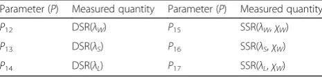
Table 7Measured quantities (P12–P17) of DSR and SSR for TCWV retrieval
Parameter (P) Measured quantity Parameter (P) Measured quantity
P12 DSR(λW) P15 SSR(λW,χW)
P13 DSR(λS) P16 SSR(λS,χW)
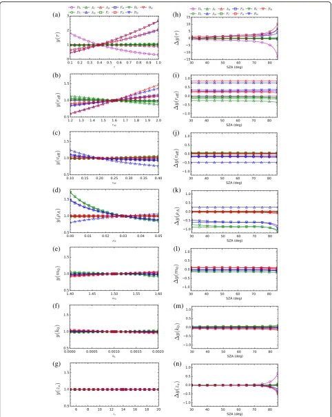
minimum to the maximum (see Table 1) and calculated the variation range ofY. Only one dust model parameter was changed at a time, with other parameters fixed to their a priori values. The results of this sensitivity ana-lysis are summarized in Fig. 5a–n.
Figure 5a–g shows the results for normalized observa-tional parameters (y) obtained with the SZA fixed at 60°, which is a typical value as indicated in the results shown below. The scales of the vertical axes are the same for these panels except for Fig. 5a. Figure 5a–g indicates that the present choice of observational parameters has led to reasonably large sensitivity (more than 30% of ob-servational parameters calculated with the a priori) toτ, reff,veff, andρA, relatively small sensitivity tom0andk0,
and much less sensitivity tozs. In Fig. 5a–d, most of the resulting curves show linear (or nearly linear) responses, though some non-linear features are seen as in the case ofD0vs.τin Fig. 5a.
In Fig. 5h–n, the results for variation range (Δy) are plotted as functions of SZA. Here, Δy stands for the maximum minus the minimum value (Δy> 0) if the ob-servational parameter increases with increasing model parameter, otherwise the minimum minus the maximum (Δy< 0). For instance, ΔD0(τ) in Fig. 5h shows the SZA
dependence of the difference between the minimum D0
and maximumD0whenτis changed between 0.1 and 1,
as indicated in Fig. 5a (for SZA = 60°). Such graphs are useful for estimating how the sensitivity changes with the time of DSR/SSR observations. Although in most cases no dependence on SZA can be seen, in some cases such asD0vs.τ, a certain increase in variation
(sensitiv-ity) is found with increasing SZA. This is ascribable to the longer path of DSR in the dust layer under large SZA conditions, namely, at dusk and dawn.
For better retrieval of each model parameter, it is re-quired for an observational parameter to have a large sensitivity to that model parameter. It is also desirable that it exhibit sensitivity solely to that specific model parameter, not being affected by other model parame-ters. For example, D0= DSR(λ0) has sensitivity solely to
τ; thus, the aerosol optical depth, τ, is well retrieved from the DSR measurement. Similarly, the dust effective radius, reff, can be retrieved from AR= SSR(λR, χA)/
SSR(λR,χ0), the hematite volume mixing ratio, ρA, from FC= SSR(λB, χF)/SSR(λR, χF), and if reff and ρA are
already known, the width parameter of size distribution, veff, can be obtained from AB= SSR(λB, χA)/SSR(λB, χ0).
Therefore, the combination of observational parameters listed in Table 4 can provide information sufficient for retrievingτ,reff,ρA, andveff. Although only limited
infor-mation on dust scale height (zs) can be obtained from our retrieval, it is necessary to include zsin our retrieval procedure so as to examine the influence ofzson the re-trieval of other dust model parameters. A detailed dis-cussion on the information content of each dust model parameter will be given later.
Error estimation for dust measurement
In the following discussion, for simplicity, it is assumed that all measured quantities (Pin Table 4) have the same relative error, and the propagation errors of observa-tional parameters (Y in Table 5) are estimated by giving a reasonably small relative error of 1%. Since random noise is considered in the measured quantities, the variance-covariance matrix of measured quantities (Sp) is assumed to be diagonal. Errors in the normalized measured quantities (p) propagate to the normalized ob-servational parameters (y) according to the Jacobian matrix Kp=∂y/∂p and the variance-covariance matrix can be calculated as Sy=KpSpKpT. Although this matrix can be non-diagonal, we retain only the diagonal ele-ments. If non-diagonal elements are included, the deter-minant becomes zero (and hence, Sy–1 cannot be calculated), since we have assumed the same relative er-rors (1%) of measured quantities. The uncertainties of the dust model parameters are not yet precisely known. Thus, we assume the standard deviations to be half of the variation range in Table 1, and the variance-covariance matrixSeis constructed by considering diag-onal elements only (i.e., [diag(Se)]
1/2
=Δx/2).
The relation between the regularization parameter (γ) of dust model parameters and the diagonal elements of AKM is plotted in Fig. 6. The averaging kernel close to 1.0 corresponds to the case that the model parameter is mostly determined by the observed DSR/SSR data while the averaging kernel being close to 0.0 is the case of the model parameter being mainly determined by the a priori data. Since observational parameters have large sensitivity to the four dust model parameters (τ,reff,veff,
and ρA), the residuals of observational parameters
Table 8Observational parameters (Y12–Y15) for TCWV retrieval
Parameter (Y) Relationship with measured quantities
Y12 D2 P12/P13 DSR(λW)/DSR(λS)
Y13 S2 P15/P16 SSR(λW,χW)/SSR(λS,χW)
Y14 D3 P12/[αP13+βP14] DSR(λW)/[αDSR(λS) +βDSR(λL)]
Y15 S3 P15/[αP16+βP17] SSR(λW,χW)/[αSSR(λS,χW) +βSSR(λL,χW)]
(a) (h)
(b) (i)
(c) (j)
(d) (k)
(e) (l)
(f) (m)
(g) (n)
increase whenγincreases in the range ofγ> 1. Although a matrix form of γ can potentially be adopted so as to enable the separate adjustment of regularization strength for each dust model parameter, here, we use the same regularization parameter ofγ= 1 for all dust model pa-rameters for the sake of simplicity. When γ= 1,zsis al-most confined to its a priori value (14 km).
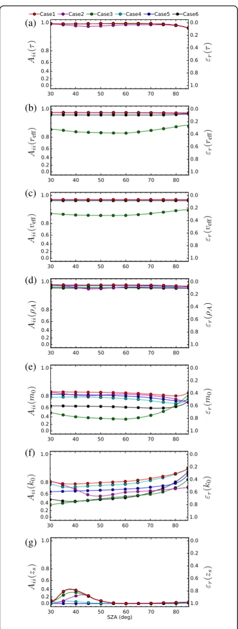
Consideration on cases with insufficient data availability
In the actual lander mission, there might be cases in which DSR/SSR cannot be observed at some specific scattering angles or accurate color ratios cannot be obtained due to reasons such as the limited dynamic range of the sensor, bad observation conditions, diffi-culty in calibration, etc. In view of such possibilities, here, we estimate propagation errors for the following six cases: case 1. Full utilization of all observational parameters; case 2. DSRs (D0, DC) are not available;
case 3. Aureoles (AC, AB, AR) are not available; case 4. Forward scattering values (FC, FB, FR) are not avail-able; case 5. Backward scattering values (BC, BB, BR) are not available; and case 6. Color ratios (DC, AC, FC, BC) are not available.
First, the diagonal elements of AKM for these six cases are shown in Fig. 7 (left scale). In case 1, the averaging kernels of τ, reff, veff, and ρA are almost in unity and those of m0 andk0 are about 0.8. Thus,
ob-servation information is well reflected in the retrieved values of these dust model parameters. On the other hand, the averaging kernels of zs are much smaller and nearly zero at SZA > 55°, which means that zs is almost confined to its a priori value. In other cases, averaging kernels are smaller as compared with case 1 and dependence on a priori is larger especially in cases 3 and 6.
Combined propagation errors of the dust model pa-rameters (Ec= [diag(Sc)]1/2) are shown in Fig. 8. For
the evaluation of retrieval errors, errors relative to the a priori values are intuitively more understandable than those relative to the variation range, and hence, here errors are expressed as values relative to both variation ranges (ΔX) and a priori values (Xa). Errors relative to a priori values are obtained from errors relative to variation range multiplied by ΔX/Xa in Table 1. The left and right scales of Fig. 8 are nor-malized so that Δx= 1 and xa= 1, respectively. In case 1, the combined propagation errors normalized with
Δx (normalized with xa) are as follows; τ: 0.5–2% (1– 4%), reff: 3% (2%), veff: 4% (5%), and ρA: 2–3% (4–6%). Compared with case 1, the total propagation errors are larger especially in the following cases; τ: case 2, reff: cases 3 and 6, veff: case 3, and ρA: cases 2, 3, and 6. As for m0 and k0, the combined propagation errors
of both parameters in case 1 are about 20% of Δx, which is 3 and 40% of xa for m0 and k0, respectively.
The errors of m0 and k0 are larger especially in case
3 (without aureole) and case 6 (without color ratio). The combined propagation error of zs is close to the
a priori error (Δx/2) since zs is almost confined to its a priori value. The percentage of a priori error in the combined propagation error is larger if the error ratio shown in Fig. 8 (right scale) is larger. The above propagation errors have been estimated with a relative measurement error of 1%, and it is expected that the propagation error is proportional to the measurement error if it is sufficiently small. Note, however, that the percentage of a priori error changes if the weight ra-tio of KxTSy–1Kx and Sa–1 changes.
Once a retrieval error occurs in a dust model param-eter, it may propagate to the other model parameters. This effect becomes significant if the non-diagonal ments of AKM are not negligible. The non-diagonal ele-ments of AKM in the above six cases are shown in Fig. 9. Since we have assumed that all of the diagonal el-ements of Sa are the same (i.e., [diag(Sa)]
1/2
=Δx/2), AKM (Aij=∂xr,i/∂xj) is symmetric and we show only ele-ments which satisfyi>jand Aij> 0.02 at one of the con-sidered SZAs. We can see that m0 and k0(xr:k0, x: m0)
are easily influenced by each other (especially in case 6). Also, in case 3, the correlation becomes larger between m0and size distribution parameters (reffandveff).
Non-spherical dust shape
Previous studies on terrestrial aerosols have shown that the differences in the shapes of coarse mode par-ticles play an important role in the spectra of DSR and SSR, since scattering patterns are dependent on the spherical (hygroscopic) or non-spherical (such as desert dust) shapes of aerosol particles. Dubovik et al. (2006) reported that the light scattering properties of desert dust aerosols in the terrestrial atmosphere can
be modeled by considering a mixture of spherical and non-spherical aerosol types. For non-spherical parti-cles, their aspect ratio distribution was estimated from a feldspar sample (Dubovik et al. 2006). Follow-ing their treatment, we assume in the present analysis that the optical properties of Martian dust can be modeled by adjusting the volume mixing ratio (ρN) of non-spherical particles to spherical particles. Variation ranges for all the observational parameters listed in Table 5 are examined by changing the value of ρN be-tween 0 and 1. The results are plotted in Fig. 10a as functions of SZA. Among the 11 observational pa-rameters, AB= SSR(λB, χA)/SSR(λB, χ0) exhibits the
largest sensitivity to ρN (Δy(ρN) = 0.15). Relatively large dependence on SZA is seen for parameters re-lated to backscattering (BR, BC, and BB). Figure 10b shows the systematic errors of retrieved dust model parameters when the wrong assumption of ρN= 0 (spherical) is adopted to analyze the observational data of dust particles that are totally non-spherical (ρN= 1). The parameters except veff and k0 have small
systematic errors (less than 15%). The parameters veff
and k0 show errors as large as 25 and 80% of their
variation ranges (~40% and 160% of their a priori values), respectively. Thus, it is desirable to take the non-sphericity of dust particles into account in the re-trieval of dust model parameters as with our dust model.
Bimodal size distribution
We have so far assumed a monomodal size distribution based on coarse mode dust particles. From the simultan-eous observation in the ultraviolet and infrared ranges by SPICAM on Mars Express, however, Fedorova et al. (2014) reported the existence of fine mode (radius 0.04– 0.07μm) as well as coarse mode (average radius 0.7μm) particles in the higher altitudes, ranging between 10 and 80 km. Therefore, in this part, we examine the influence of additional fine mode particles in our model calcula-tion. In order to reduce the number of dust model pa-rameters, we assume that the complex RI of the fine mode is the same as that of the coarse mode particles. For the coarse mode, we employ the gamma distribution of Eq. (2) with reff= 1.6 μm andveff= 0.2 as before. For
the fine mode, we follow the model given by Fedorova et al. (2014), namely, a log-normal distribution with effective
(a)
(b)
(c)
(d)
(e)
(f)
(g)
radiusr2= 0.06μm and effective variance v2= 0.1. A
log-normal distribution is given as
dN d lnr¼
1
σpffiffiffiffiffiffi2πexp −
ðlnr−lnrmodÞ2 2σ2
# "
: ð19Þ
Here,rmodis the mode radius andσis the standard
de-viation. The values of mode radius and standard deriv-ation can be calculated from the effective radius and variance as rmod=r2(v2+ 1)−5/2 andσ= [ln(v2+ 1)]1/2,
re-spectively. We parameterize the volume mixing ratio of the fine mode (ρF) between 0 (the a priori value) and 0.01.
The sensitivities of dust observation parameters to the volume mixing ratio of fine mode dust (ρF) are shown in Fig. 11a. Observational parameters such as FB, FC, BB, and BC (i.e., parameters related to SSR in the blue band except aureole) are particularly sensitive toρF.
Figure 11b shows the systematic errors of retrieved dust model parameters when the wrong assumption of ρF= 0 (monomodal) is adopted, while the true value of ρF is 0.01 (slightly bimodal). Figure 11b indicates that the magnitudes of error inρAand k0are at most 10% of
their variation range (~20% of their a priori values) even when the volume mixing ratio of fine mode is as large as 1%. Since the presence of fine mode particles in the lower Mars atmosphere has not been reported conclu-sively, it would be justified to assume the monomodal size distribution as in the present analysis. Nevertheless, to validate such a monomodal assumption, it is desirable to check the fitting result of real data to be obtained in future Mars lander missions.
Sensitivity analysis and error estimation for TCWV measurement
In a similar way as applied to the dust model parame-ters, sensitivity analysis for water vapor retrieval is made by changing the value ofcw between 0.476 and 4.76 mg/ cm2(corresponding to 100 and 1000 ppm, respectively). Figure 12 shows the resulting curves of the variation ranges (sensitivities) of the observational parameters plotted against SZA. The SZA dependencies of the sen-sitivities of D2= DSR(λW)/DSR(λS) and D3= DSR(λW)/
DSR0(λW) to cw are very similar. While D3 is sensitive
only tocw,D2exhibits large sensitivity not only tocwbut
also toτ. Thus,D3is a better parameter thanD2for the
cw retrieval, as expected from the better knowledge of the spectral intensity around the absorption band. As for SSR, both S2= SSR(λW)/SSR(λS) and S3= SSR(λW)/
SSR0(λW) exhibit similar SZA dependence of the sensi-tivities tocw, and the advantage of usingS2or S3for the
retrieval ofcw is that the magnitudes of the sensitivities are approximately three times larger than those of D2
and D3. A drawback, however, is that they show
(a)
(b)
(c)
(d)
(e)
(f)
(g)
sensitivities toτ andzsin addition to cw. Especially, the dependence onzscan be problematic, since this param-eter cannot be measured accurately through dust obser-vations. This problem is hardly improved even with three wavelengths, since the difference ofτor zs results in a change of effective optical path length due to mul-tiple scattering, and hence, the change in the amount of water vapor absorption itself. It should be pointed out, however, that we may be able to retrieve the value of zs if both DSR and SSR can be measured simultaneously. Moreover, a better prospect for zsretrieval may possibly be achieved by measuring carbon dioxide (CO2)
absorp-tion with the MAX-DOAS technique (Irie et al. 2008), since it would be relatively easy to estimate the vertical distribution of CO2, and the molecule has strong
absorp-tion bands in the near infrared region (e.g., ~1050 nm).
Fig. 10aSensitivity of dust observation parameters to the volume mixing ratio of non-spherical dust (ρN). ParameterΔyrepresents the difference between the maximum and minimum values of the normalized observational parameters whenρNis changed from 0 to 1. bSystematic error due to non-spherical dust shape. Systematic errors of normalized dust model parameters are estimated from differences between observational parameters calculated with true (1) and wrong (0) values of the volume mixing ratio of non-spherical dust (ρN)
(a)
(b)
(c)
(d)
(e)
(f)
Here, we estimate the retrieval error of TCWV (cw) when cw and dust model parameters are retrieved simultaneously. We assume a relative measurement error of 1%, and a regularization parameter γd= 1 is employed for dust model parameters. Figure 13 shows the relation between the regularization parameter (γw) of TCWV and the diagonal elements of AKM. Here, SZA is fixed at 80°. When γw= 1, the diagonal ele-ments of AKM with D2 or D3 are about 0.4 and the
influence of the a priori information is significant. Hence, we take γw= 0.06, at which the diagonal ele-ments of AKM are larger than 0.9. Weakening the regularization strength results in vulnerability to the random error of measurements, but such influence can be reduced by increasing averaging or exposure time of the camera measurement.
We consider four cases in which one ofD2, D3,S2, or
S3is used for the retrieval ofcw. The diagonal elements
of AKM for the four different cases are shown in Fig. 14 (left scale). The difference between two and three wave-lengths turns out to be insignificant. In the cases of DSR (D2,D3), the averaging kernels are around 0.7–0.9, while
in the cases of SSR (S2, S3) the averaging kernels are
about 0.98.
Fig. 12Sensitivities of water vapor observation parameters to TCWV and dust model parameters. Panels (a) - (d) show the relation betweenΔy(cw) and SZA forD2,D3,S2, andS3, respectively
Fig. 13Relation between regularization parameter (γw) of TCWV and diagonal elements of AKM
The combined propagation errors are shown in Fig. 14b. They include the contributions from both measurement errors and a priori errors according to the error ratio shown in Fig. 14a (right scale). Again, the dif-ference between two and three wavelengths is insignifi-cant. Looking around SZA = 80°, the propagation errors normalized byxaare 1.7 and 0.5 when we use DSR and SSR, respectively. This means that if we can suppress the measurement error down to 1%, SSR-based retrieval ofcwcan achieve a precision of 50% of its a priori value.
As seen above, it is expected that the combined propa-gation errors are smaller if we use SSR rather than DSR. In the case of SSR, on the other hand, the amplitudes of non-diagonal elements of AKM are larger (Fig. 15), and the retrievedcwis more affected by the retrieval error of dust model parameters (especially zs), which is consist-ent with the results of the presconsist-ent sensitivity analysis (Fig. 12). However, the error ofcw due to the error in zs is at most ~15% of the variation range (50% of the a priori value). Also, the influence of the water vapor pro-file on SSR is expected to be small for any particular value of cw. Therefore, it is advantageous to use SSR, and if available, using both SSR and DSR is desirable.
Applicability of the present algorithm
In order to check the practical applicability of our algo-rithms, we estimate the measurement noise assuming sensor specifications that can be realized with the current technology. We employ radiative transfer
simulation to estimate the minimum signal strength of SSR. The simulation conditions assumed for minimizing SSR intensity are an SZA of 80°, scattering angle of 120°, and dust optical depth of 0.1. Then, signal-to-noise (S/ N) ratio is estimated from the SSR intensity. Only the shot noise of the sensor has been considered in this cal-culation, on the assumption that the dark noise and readout noise are negligibly small.
If we assume a focal length of 10 mm, an array with 500 pixels, and a field-of-view (FOV) angle of 30°, the sizes of a sensor element and array width are calculated to be approximately 10 and 5.2 mm, respectively. A two-dimensional image sensor that fulfills such specifications is easily available. Even when the signal strength is at its
Fig. 14aDiagonal elements of AKM and error ratio of TCWV. As compared with DSR, SSR results show stronger dependence on observation data ofcwrather than a priori data.bCombined propagation errors of TCWV. The left and right scales are normalized so thatΔx= 1 andxa= 1, respectively
minimum and the exposure time is as short as 1 s, it is expected that the random noise is less than 0.5%, and hence, an S/N ratio over 200 can be attained. Actually, the exposure time can be much longer than 1 s, since a temporal resolution of 1 min, for example, is still accept-able. Therefore, the proposed scheme of DSR/SSR obser-vation is practical and achievable by means of hardware existing today.
Conclusions
We have constructed a Martian dust model in order to retrieve optical/physical properties of Martian dust from DSR/SSR spectra to be measured by a multi-wavelength environmental camera onboard a Mars lander. We have assumed that Martian dust is composed of silicate-like substrate and hematite-like inclusion. The dust shape is assumed to be spheroid with a monomodal gamma size distribution and a fixed aspect ratio distribution esti-mated from a terrestrial feldspar sample. The spatial dis-tribution of dust is homogeneous horizontally, and its concentration decreases exponentially with increasing altitude. Our Martian dust model is parameterized with seven parameters, namely, real (m0) and imaginary (k0)
parts of silicate RI, volume mixing ratio of hematite (ρA), effective radius (reff) and variance (veff) of size
distribu-tion, optical depth (τ), and scale height (zs) of extinction coefficient at a wavelength of 550 nm. On the other hand, we consider 11 observational parameters, namely, intensity of DSR at 550 nm (D0), color ratio of DSR
be-tween blue and red bands (DC), relative intensities of aureole, forward scattering, and backward scattering with respect to the SSR at the reference scattering angle for the blue and red bands (AB, AR, FB, FR,BB,BR), and color ratio of SSR (AC,FC,BC).
From the result of error analysis using simulated data, relative errors (combined propagation error from both measurement and a priori data) of dust model parame-ters, comparing them to a measurement error of 1%, have been estimated asτ: 1–4%, reff: 2%,veff: 5%,ρA: 4– 6%, m0: 3%, and k0: 40% of their a priori values. The
value ofzsis almost confined to its a priori value, due to the lack of sensitivity in our observation scheme. In-crease of retrieval error is observed when some of the observational parameters are omitted from the retrieval procedure. Such observational parameters are τ: DSR (D0, DC), reff: aureole (AC, AB, AR) and color ratio (DC,
AC, FC, BC),veff: aureole,ρA: DSR, aureole and color ra-tio,m0and k0: aureole and color ratio. If spherical shape
is employed to retrieve the dust model parameters from the observational parameters calculated for non-spherical shape, we expect a systematic error of veff as
large as 40% of its a priori value. If a monomodal gamma distribution of coarse particles is employed in finding model parameters from observational ones but the true
size distribution is bimodal containing 1% fine mode particles by volume, we expect a systematic error of ρA as large as 20% of its a priori value.
Water vapor has absorption bands inside the sensitive range of a CMOS sensor, and we can measure TCWV (cw) from absorbed amount in DSR or SSR intensity. We considered four observational parameters of spectral ra-tio (D2,D3,S2,S3) calculated with DSR or SSR at two or
three wavelengths. Using simulation, it has been con-firmed that if we use SSR instead of DSR for the obser-vational parameter, larger sensitivity can be expected, with the relative error ofcw against 1% of measurement error being 50% of its a priori value.
The measurement noise estimated with currently available sensor specifications is sufficiently small, and thus, we conclude that the proposed scheme of dust re-trieval with DSR/SSR observation is practical.
Abbreviations
AKM:Averaging Kernel Matrix; CMOS: Complementary metal-oxide semicon-ductor; DSR: Direct solar radiation; FOV: Field of view; LOS: Line of sight; MAX-DOAS: Multi-axis differential optical absorption spectroscopy; RI: Refractive index; SSR: Scattered solar radiation; SZA: Solar zenith angle; TCWV: Total column water vapor; VMR: Volume mixing ratio
Funding
This work was supported by the joint research program of CEReS, Chiba university (2015, 2016).
Authors’contributions
NM, KN, GLH, and MS proposed the topic, and conceived and designed the study. NM carried out the simulation study. NM and KN wrote the manuscript. HK contributed to editing the manuscript. HS and NO provided ideas for the study. All authors read and approved the final manuscript.
Competing interests
The authors declare that they have no competing interest.
Publisher’s Note
Springer Nature remains neutral with regard to jurisdictional claims in published maps and institutional affiliations.
Author details
1Center for Environmental Remote Sensing, Chiba University, 1-33 Yayoi-cho,
Inage-ku, Chiba-shi, Chiba 263-8522, Japan.2Department of Chemistry, Biology, and Environmental Science, Faculty of Science, Nara Women’s University, Kita-uoya Nishi-machi, Nara-shi, Nara 630-8506, Japan.
3Department of Earth Sciences, Okayama University, 3-1-1 Tsushimanaka,
Kita-ku, Okayama-shi, Okayama 700-8530, Japan.4Planetary Exploration Research Center, Chiba Institute of Technology, 2-17-1 Tsudanuma, Narashino-shi, Chiba 275-0016, Japan.5Department of Earth System Science, Faculty of Science, Fukuoka University, 8-19-1 Nanakuma, Jonan-ku, Fukuoka-shi, Fukuoka 814-0180, Japan.6Institute of Space and Astronautical Science, Japan Aerospace Exploration Agency, 3-1-1 Yoshinodai, Chuo-ku, Sagamihara-shi, Kanagawa 252-5210, Japan.
Received: 1 October 2016 Accepted: 4 June 2017
References
(2003) Mars Exploration Rover Athena Panoramic Camera (Pancam) investigation. J Geophys Res Planets 108(E12):8063. doi:10.1029/2003JE002070 Bell JF, Squyres SW, Arvidson RE, Arneson HM, Bass D, Calvin W, Farrand WH,
Goetz W, Golombek M, Greeley R, Grotzinger J, Guinness E, Hayes AG, Hubbard MYH, Herkenhoff KE, Johnson MJ, Johnson JR, Joseph J, Kinch KM, Lemmon MT, Li R, Madsen MB, Maki JN, Malin M, McCartney E, McLennan S, McSween HY, Ming DW, Morris RV, Dobrea EZN et al (2004a) Pancam multispectral imaging results from the Opportunity Rover at Meridiani Planum. Science 306(5702):1703–1709. doi:10.1126/science.1105245 Bell JF, Squyres SW, Arvidson RE, Arneson HM, Bass D, Blaney D, Cabrol N, Calvin
W, Farmer J, Farrand WH, Goetz W, Golombek M, Grant JA, Greeley R, Guinness E, Hayes AG, Hubbard MYH, Herkenhoff KE, Johnson MJ, Johnson JR, Joseph J, Kinch KM, Lemmon MT, Li R, Madsen MB, Maki JN, Malin M, McCartney E, McLennan S, McSween HY et al (2004b) Pancam multispectral imaging results from the Spirit Rover at Gusev Crater. Science 305(5685):800– 806. doi:10.1126/science.1100175
Berk A, Anderson GP, Acharya PK, Bernstein LS, Muratov L, Lee J, Fox M, Adler-Golden SM, Chetwynd JH Jr, Hoke ML, Lockwood RB, Gardner JA, Cooley TW, Borel CC, Lewis PE, Shettle EP (2006) MODTRAN5: 2006 update. In: Shen SS, Lewis PE (eds) Proceedings of SPIE 6233, Orlando, 17 April 2006.. doi:10.1117/ 12.665077
Dabrowska DD, Muñoz O, Moreno F, Ramos JL, Martínez-Frías J, Wurm G (2015) Scattering matrices of Martian dust analogs at 488 nm and 647 nm. Icarus 250:83–94. doi:10.1016/j.icarus.2014.11.024
Dlugach ZM, Korablev OI, Morozhenko AV, Moroz VI, Petrova EV, Rodin AV (2003) Physical properties of dust in the Martian atmosphere: analysis of contradictions and possible ways of their resolution. Sol Syst Res 37(1):1–19. doi:10.1023/A:1022395404115
Doicu A, Trautmann T, Schreler F (2010) Numerical regularization for atmospheric inverse problems. Springer, Heidelberg
Dubovik O, Sinyuk A, Lapyonok T, Holben BN, Mishchenko M, Yang P, Eck TF, Volten H, Muñoz O, Veihelmann B, van der Zande WJ, Leon J-F, Sorokin M, Slutsker I (2006) Application of spheroid models to account for aerosol particle nonsphericity in remote sensing of desert dust. J Geophys Res Atmos 111(D11). doi:10.1029/2005JD006619.
Ehlers K, Chakrabarty R, Moosmüller H (2014) Blue moons and Martian sunsets. Appl Opt 53(9):1808–1819. doi:10.1364/AO.53.001808
Fedorova AA, Korablev OI, Bertaux J-L, Rodin AV, Montmessin F, Belyaev DA, Reberac A (2009) Solar infrared occultation observations by SPICAM experiment on Mars-Express: simultaneous measurements of the vertical distributions of H2O, CO2 and aerosol. Icarus 200(1):96–117. doi:10.1016/j. icarus.2008.11.006
Fedorova AA, Montmessin F, Rodin AV, Korablev OI, Määttänen A, Maltagliati L, Bertaux J-L (2014) Evidence for a bimodal size distribution for the suspended aerosol particles on Mars. Icarus 231:239–260. doi:10.1016/j.icarus.2013.12.015 Flasar FM, Goody RM (1976) Diurnal behaviour of water on mars. Planet Space
Sci 24(2):161–181. doi:10.1016/0032-0633(76)90103-3
Gierasch PJ, Goody RM (1972) The effect of dust on the temperature of the Martian atmosphere. J Atmos Sci 29(2):400–402
Haberle RM, McKay CP, Schaeffer J, Cabrol NA, Grin EA, Zent AP, Quinn R (2001) On the possibility of liquid water on present-day Mars. J Geophys Res Planets 106(E10):23317–23326. doi:10.1029/2000JE001360
Hamilton VE, Christensen PR (2005) Evidence for extensive, olivine-rich bedrock on Mars. Geology 33(6):433–436. doi:10.1130/G21258.1
Hansen JE, Travis LD (1974) Light scattering in planetary atmospheres. Space Sci Rev 16(4):527–610. doi:10.1007/BF00168069
Hinson DP, Wilson RJ (2004) Temperature inversions, thermal tides, and water ice clouds in the Martian tropics. J Geophys Res Planets 109(E1). doi:10.1029/ 2003JE002129. E01002.
Hoekzema NM, Garcia-Comas M, Stenzel OJ, Grieger B, Markiewicz WJ, Gwinner K, Keller HU (2010) Optical depth and its scale-height in Valles Marineris from HRSC stereo images. Earth Planet Sci Lett 294(3–4):534–540. doi:10.1016/j. epsl.2010.02.009
Irie H, Kanaya Y, Akimoto H, Iwabuchi H, Shimizu A, Aoki K (2008) First retrieval of tropospheric aerosol profiles using MAX-DOAS and comparison with lidar and sky radiometer measurements. Atmos Chem Phys 8(2):341–350 Isaacs RG, Wang W-C, Worsham RD, Goldenberg S (1987) Multiple scattering lowtran
and fascode models. Appl Opt 26(7):1272–1281. doi:10.1364/AO.26.001272 Komguem L, Whiteway JA, Dickinson C, Daly M, Lemmon MT (2013) Phoenix
LIDAR measurements of Mars atmospheric dust. Icarus 223(2):649–653. doi: 10.1016/j.icarus.2013.01.020
Lemmon MT, Wolff MJ, Smith MD, Clancy RT, Banfield D, Landis GA, Ghosh A, Smith PH, Spanovich N, Whitney B, Whelley P, Greeley R, Thompson S, Bell JF, Squyres SW (2004) Atmospheric imaging results from the Mars exploration rovers: Spirit and Opportunity. Science 306(5702):1753–1756. doi: 10.1126/science.1104474
Lemmon MT, Smith PH, Shinohara C, Tanner R, Woida P, Shaw A, Hughes J, Reynolds R, Woida R, Penegor J, Oquest C, Hviid SF, Madsen MB, Olsen M, Leer K, Drube L, Morris RV, Britt DT (2008) The Phoenix Surface Stereo Imager (SSI) Investigation. Lunar and planetary science conference, League City, pp 10–14, March 2008
Levoni C, Cervino M, Guzzi R, Torricella F (1997) Atmospheric aerosol optical properties: a database of radiative characteristics of different components and classes. Appl Opt 36(30):8031–8041
Malin MC, Caplinger MA, Edgett KS, Ghaemi FT, Ravine MA, Schaffner JA, Baker JM, Bardis JD, Dibiase DR, Maki JN, Willson RG, Bell JF, Dietrich WE, Edwards LJ, Hallet B, Herkenhoff KE, Heydari E, Kah LC, Lemmon MT, Minitti ME, Olson TS, Parker TJ, Rowland SK, Schieber J, Sullivan RJ, Sumner DY, Thomas PC, Yingst RA (2010) The Mars Science Laboratory (MSL) Mast-mounted Cameras (Mastcams) flight instruments. Lunar and planetary science conference, Woodlands, pp 1–5, March 2010
Manago N, Kuze H (2010) Determination of tropospheric aerosol characteristics by spectral measurements of solar radiation using a compact, stand-alone spectroradiometer. Appl Opt 49(8):1446–1458. doi:10.1364/AO.49.001446 Manago N, Miyazawa S, Bannu KH (2011) Seasonal variation of tropospheric
aerosol properties by direct and scattered solar radiation spectroscopy. J Quant Spectrosc Radiat Transf 112(2):285–291. doi:10.1016/j.jqsrt.2010.06.015 Markiewicz WJ, Sablotny RM, Keller HU, Thomas N, Titov D, Smith PH (1999)
Optical properties of the Martian aerosols as derived from Imager for Mars Pathfinder midday sky brightness data. J Geophys Res Planets 104(E4):9009– 9017. doi:10.1029/1998JE900033
Millour E, Forget F, Spiga A, Colaitis A, Navarro T, Madeleine J-B, Chauffray J-Y, Montabone L, Lopez-Valverde MA, Gonzalez-Galindo F, Lefevre F,
Montmessin F, Lewis SR, Read PL, Desjean M-C, Huot J-P (2012) Mars Climate Database version 5. European planetary science congress, Madrid, pp 23–28, September 2012
Mishchenko MI, Travis LD (1998) Capabilities and limitations of a current FORTRAN implementation of the T-matrix method for randomly oriented, rotationally symmetric scatterers. J Quant Spectrosc Radiat Transf 60(3):309– 324. doi:10.1016/S0022-4073(98)00008-9
Moore CA, Moores JE, Lemmon MT, Rafkin SCR, Francis R, Pla-García J, Haberle RM, Zorzano M-P, Martín-Torres FJ, Burton JR (2016) A full Martian year of line-of-sight extinction within Gale Crater, Mars as acquired by the MSL Navcam through sol 900. Icarus 264:102–108. doi:10.1016/j.icarus.2015.09.001 Moores JE, Lemmon MT, Smith PH, Komguem L, Whiteway JA (2010) Atmospheric
dynamics at the Phoenix landing site as seen by the Surface Stereo Imager. J Geophys Res Planets 115(E1). doi:10.1029/2009JE003409. E00E08
Moriyama S (1975) Effects of dust on radiation transfer in the Martian atmosphere, (2). J Meteor Soc Japan 53(3):214–221
Patterson WR, Huck FO, Wall SD, Wolf MR (1977) Calibration and performance of the Viking Lander cameras. J Geophys Res 82(28):4391–4400. doi:10.1029/ JS082i028p04391
Pike WT, Staufer U, Hecht MH, Goetz W, Parrat D, Sykulska-Lawrence H, Vijendran S, Madsen MB (2011) Quantification of the dry history of the Martian soil inferred from in situ microscopy. Geophys Res Lett 38(24). doi:10.1029/ 2011GL049896
Pollack JB, Colburn D, Kahn R, Hunter J, Van Camp W, Carlston CE, Wolf MR (1977) Properties of aerosols in the Martian atmosphere, as inferred from Viking Lander imaging data. J Geophys Res 82(28):4479–4496. doi:10.1029/ JS082i028p04479
Pollack JB, Colburn DS, Flasar FM, Kahn R, Carlston CE, Pidek D (1979) Properties and effects of dust particles suspended in the Martian atmosphere. J Geophys Res Solid Earth 84(B6):2929–2945. doi:10.1029/JB084iB06p02929 Pollack JB, Ockert-Bell ME, Shepard MK (1995) Viking Lander image analysis of
Martian atmospheric dust. J Geophys Res Planets 100(E3):5235–5250. doi:10. 1029/94JE02640
Querry MR (1985) Optical constants., Technical Report AD-A158-623, DTIC Document
Rodgers CD (2000) Inverse methods for atmospheric sounding: theory and practice vol 2. World scientific, Singapore
Smith MD (2008) Spacecraft observations of the Martian atmosphere. Annu Rev Earth Planet Sci 36(1):191–219. doi:10.1146/annurev.earth.36.031207.124334 Smith MD (2009) THEMIS observations of Mars aerosol optical depth from
2002–2008. Icarus 202(2):444–452. doi:10.1016/j.icarus.2009.03.027 Smith PH, Lemmon M (1999) Opacity of the Martian atmosphere measured by
the imager for Mars Pathfinder. J Geophys Res Planets 104(E4):8975–8985. doi:10.1029/1998JE900017
Smith PH, Tomasko MG, Britt D, Crowe DG, Reid R, Keller HU, Thomas N, Gliem F, Rueffer P, Sullivan R, Greeley R, Knudsen JM, Madsen MB, Gunnlaugsson HP, Hviid SF, Goetz W, Soderblom LA, Gaddis L, Kirk R (1997) The imager for Mars Pathfinder experiment. J Geophys Res Planets 102(E2):4003–4025. doi:10. 1029/96JE03568
Smith PH, Tamppari LK, Arvidson RE, Bass D, Blaney D, Boynton WV, Carswell A, Catling DC, Clark BC, Duck T, DeJong E, Fisher D, Goetz W, Gunnlaugsson HP, Hecht MH, Hipkin V, Hoffman J, Hviid SF, Keller HU, Kounaves SP, Lange CF, Lemmon MT, Madsen MB, Markiewicz WJ, Marshall J, McKay CP, Mellon MT, Ming DW, Morris RV, Pike WT, Renno N, Staufer U, Stoker C, Taylor P, Whiteway JA, Zent AP (2009) H2O at the Phoenix landing site. Science 325(5936):58–61. doi:10.1126/science.1172339
Stamnes K, Tsay S-C, Wiscombe W, Jayaweera K (1988) Numerically stable algorithm for discrete-ordinate-method radiative transfer in multiple scattering and emitting layered media. Appl Opt 27(12):2502–2509. doi:10. 1364/AO.27.002502
Thomas N, Markiewicz WJ, Sablotny RM, Wuttke MW, Keller HU, Johnson JR, Reid RJ, Smith PH (1999) The color of the Martian sky and its influence on the illumination of the Martian surface. J Geophys Res Planets 104(E4):8795–8808. doi:10.1029/98JE02556
Titov DV, Markiewicz WJ, Thomas N, Keller HU, Sablotny RM, Tomasko MG, Lemmon MT, Smith PH (1999) Measurements of the atmospheric water vapor on Mars by the imager for Mars Pathfinder. J Geophys Res Planets 104(E4):9019–9026. doi:10.1029/1998JE900046
Tomasko MG, Doose LR, Lemmon M, Smith PH, Wegryn E (1999) Properties of dust in the Martian atmosphere from the imager on Mars Pathfinder. J Geophys Res Planets 104(E4):8987–9007. doi:10.1029/1998JE900016 Whiteway JA, Komguem L, Dickinson C, Cook C, Illnicki M, Seabrook J, Popovici V,
Duck TJ, Davy R, Taylor PA, Pathak J, Fisher D, Carswell AI, Daly M, Hipkin V, Zent AP, Hecht MH, Wood SE, Tamppari LK, Renno N, Moores JE, Lemmon MT, Daerden F, Smith PH (2009) Mars water-ice clouds and precipitation. Science 325(5936):68–70. doi:10.1126/science.1172344
Wolff MJ, Smith MD, Clancy RT, Arvidson R, Kahre M, Seelos F, Murchie S, Savijärvi H (2009) Wavelength dependence of dust aerosol single scattering albedo as observed by the Compact Reconnaissance Imaging Spectrometer. J Geophys Res Planets 114(E2). doi:10.1029/2009JE003350. E00D04.