R E S E A R C H
Open Access
Effect of image registration on longitudinal
analysis of retinal nerve fiber layer thickness of
non-human primates using Optical Coherence
Tomography (OCT)
Shuang Liu
1,4*, Anjali Datta
2, Derek Ho
1, Jordan Dwelle
1, Daifeng Wang
2, Thomas E Milner
1,
Henry Grady Rylander III
1and Mia K Markey
1,3Abstract
Background:In this paper we determined the benefits of image registration on estimating longitudinal retinal nerve fiber layer thickness (RNFLT) changes.
Methods:RNFLT maps around the optic nerve head (ONH) of healthy primate eyes were measured using Optical Coherence Tomography (OCT) weekly for 30 weeks. One automatic algorithm based on mutual information (MI) and the other semi-automatic algorithm based on log-polar transform cross-correlation using manually segmented blood vessels (LPCC_MSBV), were used to register retinal maps longitudinally. We compared the precision and recall between manually segmented image pairs for the two algorithms using a linear mixed effects model.
Results:We found that the precision calculated between manually segmented image pairs following registration by LPCC_MSBV algorithm is significantly better than the one following registration by MI algorithm (p < <0.0001). Trend of the all-rings and temporal, superior, nasal and inferior (TSNI) quadrants average of RNFLT over time in healthy primate eyes are not affected by registration. RNFLT of clock hours 1, 2, and 10 showed significant change over 30 weeks (p = 0.0058, 0.0054, and 0.0298 for clock hours 1, 2 and 10 respectively) without registration, but stayed constant over time with registration.
Conclusions:The LPCC_MSBV provides better registration of RNFLT maps recorded on different dates than the automatic MI algorithm. Registration of RNFLT maps can improve clinical analysis of glaucoma progression.
Keywords:Retinal nerve fiber layer thickness, Glaucoma, Image registration
Background
Estimation of retinal nerve fiber layer thickness (RNFLT) is an important step in both glaucoma diagnosis and de-tection of glaucoma progression. RNFLT can be object-ively and quantitatobject-ively measured by Optical Coherence Tomography (OCT). Because RNFLT maps measured by OCT are highly correlated with visual field loss [1-3], OCT can be used to assist in glaucoma diagnosis and longitudinal detection of glaucoma progression.
Studies suggest higher repeatability and reproducibility in measuring RNFLT of healthy and glaucomatous eyes with commercially available spectral-domain OCT com-pared to time-domain OCT instrumentation [4-6]. How-ever, causes of measurement variability for example, manual placement of the scan circle by the instrument operator and patient eye rotation during successive mea-surements, remain problematic. Features of RNFLT such as temporal, superior, nasal and inferior (TSNI) quad-rants averages, and 12 clock hour sector averages have been analyzed in clinical studies for glaucoma diagnosis [7-9]. In monitoring glaucoma progression, small changes of RNFLT features might be missed and false changes of RNFLT features might be detected because of misalignment
* Correspondence:ShuangLiu@utexas.edu 1
Department of Biomedical Engineering, The University of Texas at Austin, Austin, TX 78712, USA
4
Present address: Clinical Neuroscience Imaging Center (CNIC), Department of Neurology, Yale School of Medicine, New Haven, CT 06510, USA Full list of author information is available at the end of the article
© 2015 Liu et al.; licensee BioMed Central. This is an Open Access article distributed under the terms of the Creative Commons Attribution License (http://creativecommons.org/licenses/by/4.0), which permits unrestricted use, distribution, and
of successive RNFLT maps. Therefore, accurate registration of maps recorded at different OCT imaging sessions is de-sired for assessment of glaucoma progression [10-12]. Re-cently, methods including tracking systems and scan alignments based on the optic nerve head (ONH) have been developed to improve image registration and RNFLT measurement reproducibility [12,13]. Some of the latest versions of commercially available spectral domain OCT software also incorporate methods to enable serial analysis of RNFLT changes. For example, the Spectralis OCT (Heidelberg Engineering, Heidelberg, Germany) uses a system to track eye movements and enable “real-time” registration. The OCT software package RTVue FD-OCT (Optovue, Inc., Fremont, CA) uses post-processing methods based on baseline images to enable registra-tion [14]. Most of the recent registraregistra-tion methods for OCT scans are based on blood vessel structures or mu-tual information (MI) of fundus images [15-17]. Previ-ous studies have shown that evaluation of RNFLT might be affected by variations in the position of the scan circle of measurements around the optic nerve that can compromise measurement reproducibility in eyes of healthy human subjects [18,19]. However, no study has been reported on whether image registration can improve longitudinal RNFLT evaluation in healthy eyes, and which RNFLT features may be more sensitive to misalignment of RNFLT maps recorded on different dates.
In this longitudinal study, we presented and compared an automatic algorithm based on MI and a semi-automatic algorithm based on log-polar transform cross-correlation using manually segmented blood vessels (LPCC_MSBV) for registration of RNFLT maps from a spectral domain OCT instrument of healthy non-human primates. We chose to investigate MI and LPCC_MSBV algorithms because they were demonstrated as two ro-bust approaches for retinal image registration [20-23]. We evaluated changes in 17 different RNFLT features calculated from the RNFLT maps (all rings average, TSNI quadrants average and 12 clock hour sectors aver-age) with and without registration over a 30-week time period.
Methods
Experimental design
Retinal nerve fiber layer (RNFL) imaging was performed on three macaque monkeys: two cynomolgus monkeys (macaca fascicularis), and one rhesus macaque monkey (macaca mulatta). One eye (OS) in each primate was followed over a period of 30 weeks during which weekly OCT imaging and measurement sessions were performed to assess the IOP and record RNFL thickness [24].
All studies performed in this work were done under the direction of The University of Texas Institutional
Animal Care and Use Committee, which followed an ap-proved protocol (#08013001), and adhered to the ARVO Statement for the Use of Animals in Ophthalmic and Vision Research. The OCT system utilized to image the primates is a custom-built tabletop research instrument Polarization Sensitive OCT (PS-OCT) with free-space optics constructed for the purpose of this study [24,25]. Comparison of this OCT system to RTVue and Cirrus OCT systems is shown in the Additional file 1: Table S1. The PS-OCT system uses a swept laser source (Santec, HSL 1000) with a 1 μm center wavelength and axial resolution of 12 μm. Lateral resolution is approximately 25 μm. Average incident power on the primate cornea was 1.13 mW. The head of the anesthetized primate was gently secured in a cradle with angular position con-trolled by two goniometers. Eye orientation was manipu-lated with sutures at the limbus to bring the ONH into the center of the field of view, and resulted in significant variation in the globe orientation between imaging ses-sions. Moreover, placement of the scan circle by the in-strument operator was not repeatable between imaging sessions and introduced some translational misalignment in RNFLT maps.
The left eye of each primate was imaged every week over a 30-week time period. Poor quality scans such as scans with A-scans affected by eye blinking or cases when the RNFL is out of the effective imaging depth were rejected by the instrument operator. There were 8 measurements for primate 1; 16 measurements for pri-mate 2; 16 measurements for pripri-mate 3 over the 30 weeks selected for the analysis. Two scanning pat-terns were used to generate retinal maps. For each pri-mate eye, one raster scan with best quality (minimum eye movement and best contrast) was performed on a 3 × 3 mm2 square area centered on the ONH. Each raster scan was comprised of 100 scans and each B-scan consisted of 256 A-B-scans. We created a raster B-scan fundus image by summing pixels of all the B-scan im-ages and rescaled it to 256 × 256 pixels, and used it as the reference image for the respective primate eye. A second scanning pattern was a continuous ring scan pat-tern that contained 100 equally spaced ring B-scans cen-tered on the ONH with ring diameters ranging from 1.5 mm to 3.0 mm. Each B-scan contained 100 A-scans. Data recorded from continuous ring scans were used to create an RNFL thickness map of each eye. Fundus im-ages of continuous ring scans were created by summing pixels of all the B-scan images along the axial direction for registration purposes as target images (Figure 1).
Retinal nerve fiber layer thickness map and feature calculation
automatically detect RNFL boundaries in each B-scan of continuous ring scans [25,26]. After RNFL boundary de-tection, an expert on OCT retinal image evaluation visu-ally inspected the boundaries overlaid on each B-scan to correct any misidentified boundaries. RNFLT values were then imported into MATLAB (The Mathworks, Natick, MA) for RNFL feature calculation. The most widely used feature parameters were computed including the all-rings average thickness, TSNI quadrants average thick-nesses, and each of the 12-clock hour RNFLT averages according to the OD clock-wise hours (Figure 2). Fea-ture values were calculated on RNFLT maps before and after registration.
Registration and evaluation method
One fundus image created from the raster scan was used as a reference image for each primate eye. All fundus images of continuous ring scans were target images and registered against this baseline image to ensure align-ment of all RNFL thickness maps obtained with the con-tinuous ring scan method. We applied two registration algorithms, MI and LPCC_MSBV) algorithms. The process of applying MI and LPCC_MSBV algorithms, and evaluation of precision and recall are shown in a
flowchart (Figure 3). The original reference and target intensity images were used for the MI algorithm to de-termine the best transformation parameters to align the reference and target image pair. The manually seg-mented blood vessel images from reference and target images (e.g., Figure 1) were used for the LPCC_MSBV algorithm to find the best transformation factors to align the reference and target image pair. Precisions and re-calls between manually segmented blood vessels of refer-ence and target image pairs were used to evaluate the alignment between image pairs before and after registra-tion. Details of the algorithms and evaluation process are described in the following sections.
Mutual information algorithm
rotation and scaling. The MI between a reference (A) tar-get (B) image pair is defined as:
MIðA;BÞ ¼H Að Þ þH Bð Þ–H Að ;BÞ ð1Þ
WhereH(A) andH(B) are the Shannon entropies of the reference (A) and target (B) images, respectively, defined as
Hð Þ ¼X −X
N
i¼1
p xð Þi logp xð Þi ð2Þ
Where p(xi) is the probability of occurrence of the
intensity valuexiin the image. Similarly,H(A,B) is the
joint Shannon entropy of images A and B, defined as
HðA;BÞ ¼−X
i;j
p ið Þ;j logð Þi;j ð3Þ
Where p(i, j) is the joint probability of the image in-tensity pairs in the joint histogram of images A and B. Two images were considered registered whenMI (A,B) had a maximum value with respect to the linear trans-formation parameters.
We performed the MI registration in two major steps: a coarse registration step followed by a fine registration step. For coarse registration, we translated the target image from −25 to 25 pixels (approximately 0.15 mm) in both x and y directions with an interval of 5 pixels (approximately 0.03 mm), and rotated the image−10 to 10 degrees in 2 degree intervals until maximum MI be-tween the reference and target images was obtained. To
Figure 3Flowchart diagramming the application of MI and LPCC_MSBV algorithms.Reference and target intensity images are used for the MI algorithm to find the transformation parameters (translation, rotation, scaling) to register the image pair. The manually segmented blood vessel images of the reference and target images are used for the LPCC_MSBV algorithm to find the transformation parameters (translation, rotation, scaling) to register the image pair. The precisions and recalls between manually segmented blood vessels in reference and target image pairs before registration (bottom left), after MI registration (upper right), and after LPCC_MSBV registration (lower right) are calculated. The LPCC_MSBV transformation parameters are used to register RNFLT maps.
RNFL
reduce time for coarse registration, larger search inter-vals were used compared to those used subsequently in fine registration. Performing three transformations sim-ultaneously helped to prevent the algorithm from stal-ling in a local maximum, which was more common if each type of transformation were to be performed sep-arately. The coarse transformation parameters that pro-vided the maximum MI were found and performed on the target image before fine registration.
In fine registration, all transformation parameters, translation, rotation and scaling were performed separ-ately with smaller search intervals to maximize MI. We first did a scaling search for a scale factor between 0.85 to 1.15 with an interval of 0.01, then varied x-translation factor from −20 pixels to 20 pixels (approximately 0.12 mm) with an interval of 1 pixel (approximately 0.006 mm), then y-translation factor from −20 pixels to 20 pixels with an interval of 1 pixel, then rotation factor from −20 to 20 degrees with an interval of 0.1 degrees, and finally scaling again with search radius between 0.85 to 1.15 with an interval of 0.01.
Log-polar transform based cross-correlation algorithm RNFLT maps recorded on different days were also regis-tered to the reference image using LPCC_MSBV algo-rithm [23]. First, we segmented the blood vessels in the original intensity reference and target images manually. Blood vessel images were mapped into log-polar coordi-nates, so that rotation and scaling in the original image corresponded to translation in log-polar images. In polar space, the translational factor in the angle direction cor-responded to a rotational factor. In addition, consider a scaling factor, a, between the images, such that (x, y) in one image maps to (ax, ay) in the other. In log space, (x, y)→(logx, logy)and (ax,ay)→(logx+ loga, logy+ log
a), so translational shifts corresponded to scaling. Log-polar transformed images were then cross-correlated to determine the scaling and rotation factors. Because spatial-domain calculations, unlike frequency-domain computations, are not translation invariant, the log-polar transform and subsequent cross-correlation was com-pleted for all possible choices of origin within a limited search area in the reference image. When the maximum cross-correlation was found, the choice of origin corre-sponded to translation and shifts in log-polar space cor-responded to scaling and rotation. To speed-up the LPCC_MSBV algorithm, search for the maximum was completed at two resolution levels, using the parameters from the coarser level as an estimate of the parameters for the finer level.
Because the OCT instrument operator approximately centered the scan ring over the ONH before recording data, images are roughly aligned, and registration is achieved within a limited range of translation factors.
Translation factors between image pairs were limited to 40 pixels (approximately 0.23 mm) to improve registration speed. For coarse registration, the images were subsam-pled to 1/4th the size, yielding 128 × 128 pixel images with 20 × 20 pixel (approximately 0.23 × 0.23 mm) search areas corresponding to x- and y-translation factors between−10 and 10 pixels (approximately 0.12 mm). Log-polar trans-forms of the target images were then cross-correlated with the log-polar transforms of the reference image.
To reduce computation time, all cross-correlations were calculated using the Fast Fourier Transform (FFT). The cross-correlation was linear in the scaling direction, but circular in the rotation direction. Therefore, the log-polar transforms of the images were zero-padded along the scaling axis, but not the rotation axis.
The optimal scaling, rotation, and translation parame-ters determined from these cross-correlations were then applied to the target image before fine registration. For fine registration, the 512 × 512 pixel blood vessel images were used, and the translation factors were limited to−4 and 4 pixels (approximately 0.02 mm). The linear trans-formation was computed as in coarse registration using log-polar transforms and cross-correlations.
Manual segmentation of blood vessels
Manual segmentation of blood vessel images was needed for two aspects of this study. First, blood vessel segmen-tation is a necessary pre-processing step for registration using the LPCC_MSBV algorithm. Second, we used the manual segmented blood vessels for calculation of preci-sion, and recall of reference-target image pairs to evalu-ate performance of MI and LPCC_MSBV algorithms.
Segmentation of the blood vessels in both raster and con-tinuous ring scan fundus images were completed manually. Using a tablet PC, the five widest blood vessels with branches in each fundus image were manually annotated.
Evaluation of the registration results
The MI and LPCC_MSBV algorithms were evaluated in terms of precision and recall between manually segmented reference, and target image pairs before and after registra-tion. The overlapped scanning region of reference and
target images was used for calculation of precision and recall. Precision and recall are defined as:
precision¼N NTP
TPþNFP ð4Þ
recall¼N NTP
TPþNFN ð5Þ
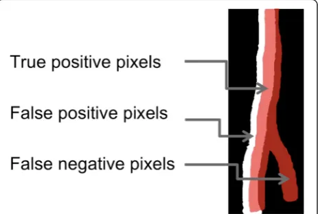
Where NTP is the number of overlapping blood vessel
pixels in reference and target images (true positives).NFPis No Registration LPCC_MSBV Registration MI Registration
Figure 5Overlap of the reference and target images.The reference image is shown as the gray scale intensity image. The target image is shown as transparent yellow lines in order to clearly demonstrate the overlap area. The overlap of the two images is shown before registration (left), after LPCC_MSBV registration (middle) and after MI registration (right).
the number of blood vessel pixels in the target image, but not in the reference image (false positives).NFNis the number of
blood vessel pixels in the reference image, but not target image (false negatives) (Figure 4). The algorithm with better performance was used for registration of RNFLT maps.
Statistical analysis
Linear mixed-effects models were used for longitudinal evaluation of estimated RNFL parameters to capture both the similarity (fixed effect) and variations (random effects) among the three primates. Linear mixed-effects models also provided unbiased analysis of balanced and unbalanced repeated-measurement data, which was con-sistent with our experiment design. We used the nlme package (R package version 3.1-104) [27] of R statis-tical programming language (v2.13.10 07/08/2011; http://www.R-project.org/, R Development Core Team, 2011, R Foundation for Statistical Computing, Vienna, Austria) and R studio (v0.94, 06/15/2011, RStudio, Inc.) for implementing the linear mixed-effects models.
We first evaluated whether the precision and recall calcu-lated for registered image pairs by MI and LPCC_MSBV al-gorithms were significantly improved compared with no registration. We also used the precision and recall of image pairs registered by MI and LPCC_MSBV algorithms to compare the performance of these two algorithms. We used the following linear mixed effects model to evaluate the significance for the pairwise comparisons:
Ti;t¼Tavgþbiþγregi;tþεi;t ð6Þ
Where Ti,tis precision or recall of the ithprimate con-trol eye on daytsince the beginning of the study, Tavgis the mean precision or recall across all the eyes.biis a
ran-dom effect representing the deviation from Tavgfor the ith primate eye, normally distributed with zero-mean and standard deviationδb;regi,tis a binary variable
represent-ing with (regi,t= 1) or without registration (regi,t= 0) for
the ithprimate control eye on day t when the model was used for comparison of precision and recall, with and without registration. When the model was used for com-parison of precision and recall of image pairs registered by MI and LPCC_MSBV algorithms,regi,tis a binary variable
representing the algorithm used for the ithprimate control eye on day t (regi,t= 0 for MI algorithm; regi,t= 1 for
LPCC_MSBV algorithm).γis the slope forregi,t;εitis a
random effect representing the deviations in precision or recall on day tof the ithprimate eye from the mean precision or recall of the ith primate eye, and normally distributed with zero-mean and standard deviationδε.
We investigated whether registration will affect the evaluation of RNFL thickness over time in this longitudinal study for healthy eyes. The following linear mixed effects model was applied,
RNFLTi;t¼ a1þβi
þa2tþξi;t ð7Þ
In the mixed effects model, RNFLTi,tis a feature value in RNFLT maps of the eye of the ith primate on day t since the beginning of the study. The intercept α1 and the mean slopeα2for number of daystare fixed effects. The random effect is the intercept βi for ith primate, which is normally distributed with zero-mean and stand-ard deviation δ. ξi,t is the random error component for the itheye on day t, and assumed to be normally distrib-uted with a mean of zero and standard deviationδe.
Results and discussion
Comparison of MI and LPCC_MSBV algorithms
One example of overlap of the reference image and tar-get image before and after MI and LPCC_MSBV regis-tration is shown in Figure 5. By visual inspection, we can see that the overlap of the reference and target images is improved after both MI and LPCC_MSBV registration. Precision and recall were used to evaluate quality of registration results before and after application of MI and LPCC_MSBV algorithms (Figure 6). We used the linear mixed effects model described in Equation 6 to compare precision and recall values before vs. after registration and precision and recall values after regis-tration by MI algorithm vs. LPCC_MSBV algorithm.
Table 1 Results of comparing precision and recall values of before registration (regi,t= 0) vs. after MI registration
(regi,t= 1)
Evaluation Linear mixed effects model coefficients and p values
Intercept p value for intercept
Slope of regi,t
p value for slope
Precision 0.2488 <<0.0001 0.4972 <<0.0001
Recall 0.2332 <<0.0001 0.6588 <<0.0001
Table 2 Results of comparing precision and recall values of before registration (regi,t= 0) vs. after registration by
LPCC_MSBV algorithm (regi,t= 1)
Evaluation Linear mixed effects model coefficients and p values
Intercept p value for intercept
Slope of regi,t
p value for slope
Precision 0.2453 <<0.0001 0.5829 <<0.0001
Recall 0.2323 <<0.0001 0.6905 <<0.0001
Table 3 Results of comparing precision and recall values of registration by MI algorithm (regi,t= 0) vs. LPCC_MSBV
algorithm (regi,t= 1)
Evaluation Linear mixed effects model coefficients and p values
Intercept p value for intercept
Slope of regi,t
p value for slope
Precision 0.7388 <<0.0001 0.0857 <<0.0001
Precision and recall following registration by either the MI or LPCC_MSBV algorithms were significantly better than that before registration (p < <0.0001, Tables 1 and 2). Thus, either the MI or LPCC_MSBV registration algorithm could significantly improve alignment of reference and target im-ages. Precision of the LPCC_MSBV algorithm was signifi-cantly higher than that of the MI algorithm (p < <0.0001, Table 3). Recalls of the MI and LPCC_MSBV algorithms were not significantly different (p = 0.0571, Table 3). Inas-much as the results suggest that the LPCC_MSBV algorithm performs slightly better than the MI algorithm on recorded primate images, we used the LPCC_MSBV algorithm to register maps for analysis of RNFLT versus time.
Analysis of RNFL thickness over time with and without registration
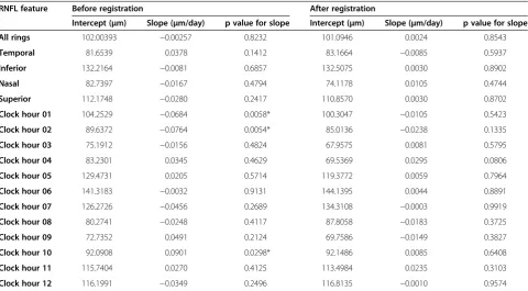
We used a linear mixed effects model (Equation 7) to evaluate whether changes in RNFLT features occurred during the study duration. Before registration, RNFLT features are calculated in each map at each date. After registering all target images to a corresponding reference image using the LPCC_MSBV algorithm, we co-aligned all RNFLT maps, and used the overlapped region of all RNFLT maps from different dates to calculate the RNFLT feature parameter values. We found that prior to registra-tion, three RNFLT features (1, 2, and 10 clock hour sectors
averages) out of seventeen features we evaluated showed significant change during the study (Figure 7 and Table 4). Before registration, one and two o’clock hour sectors aver-age RNFLT showed a significant decrease (p = 0.0058 for one o’clock hour and p = 0.0054 for two o’clock hour). Before registration, ten o’clock hour sector average in-creased significantly during the study duration (p = 0.0298). Other RNFLT features showed no change over the study duration. However, after registration, all RNFLT features, all model slopes of RNFLT feature vs. time are not sig-nificantly different from zero, suggesting that all thick-ness feature parameter values are constant over the time course of the study (Table 4). Since for healthy eyes, we would not expect the RNFL thickness to change significantly during the six months study duration [28], we concluded that consistency of RNFLT feature parameters improved after registration. The results suggest that regis-tration can remove artifacts introduced by misalignment of RNFLT maps especially in more detailed features like 12 o’clock hour sector average. Overall, the clock hour features of RNFLT are more sensitive to mis-registration artifacts compared to the all-rings average and TSNI quadrants average.
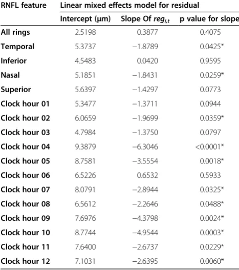
Moreover, we also compared the residuals of the linear mixed effect model before registration and after registra-tion using the LPCC_MSBV algorithm (Table 5). We
Table 4 Comparison of changes in RNFL features over time before and after registration
RNFL feature Before registration After registration
Intercept (μm) Slope (μm/day) p value for slope Intercept (μm) Slope (μm/day) p value for slope
All rings 102.00393 −0.00257 0.8232 101.0946 0.0024 0.8543
Temporal 81.6539 0.0378 0.1412 83.1664 −0.0085 0.5937
Inferior 132.2164 −0.0081 0.6857 132.5075 0.0030 0.8902
Nasal 82.7397 −0.0167 0.4794 74.1178 0.0105 0.4744
Superior 112.1748 −0.0280 0.2417 110.8570 0.0030 0.8702
Clock hour 01 104.2529 −0.0684 0.0058* 100.3047 −0.0105 0.5423
Clock hour 02 89.6372 −0.0764 0.0054* 85.0136 −0.0238 0.1335
Clock hour 03 75.1912 −0.0156 0.4824 67.9575 0.0081 0.5795
Clock hour 04 83.2301 0.0345 0.4629 69.5369 0.0295 0.0806
Clock hour 05 129.4731 0.0205 0.5714 119.3772 0.0059 0.7964
Clock hour 06 141.3183 −0.0032 0.9131 144.1395 0.0044 0.8891
Clock hour 07 126.2726 −0.0456 0.2689 134.3108 −0.0003 0.9919
Clock hour 08 80.2741 −0.0248 0.4117 87.8058 −0.0183 0.3725
Clock hour 09 72.7352 0.0491 0.2124 69.7586 −0.0149 0.3827
Clock hour 10 92.0908 0.0901 0.0298* 92.1486 0.0085 0.6408
Clock hour 11 115.7404 0.0270 0.4125 113.4984 0.0235 0.3103
Clock hour 12 116.1991 −0.0349 0.2496 116.8135 −0.0010 0.9574
A linear mixed effects model is used to estimate the change in RNFL features over time. Coefficients and the p values of the coefficients of the linear mixed effects model of RNFL features vs. days before registration and after registration by LPCC_MSBV algorithm are shown in this table. The intercept represents the magnitude of RNFL thickness and, therefore, the p values for intercepts are all zero indicating that the thickness is non-zero. The slopes represent the change of RNFL thickness features over time. The p values for the slopes are shown in the table.
found that for most RNFLT features, the magnitude of residuals of the linear mixed effects model were signifi-cantly decreased after registration (slopes were negative and p values were smaller than 0.05; marked with“*” in Table 5). Therefore, registration reduces the measure-ment error.
Conclusions
In this study, we investigated benefits of image registration on estimation of longitudinal RNFLT changes in non-human primate eyes. We compared the performance of MI and LPCC_MSBV algorithms. Precision and recall cal-culated between manually segmented blood vessel image pairs were used for comparison with that determined after applying LPCC_MSBV and MI algorithms. Results in-dicate that application of either MI or LPCC_MSBV al-gorithms improves the alignment between target and reference images compared to no registration. The preci-sion after registration by the LPCC_MSBV algorithm is significantly higher than that after registration by the MI algorithm. Recalls following registration by either MI or LPCC_MSBV algorithms are similar. The computation time of the LPCC_MSBV algorithm was five-times faster than that of the MI algorithm. However, this computation
time does not include the pre-processing time required to manually segment the blood vessels before applica-tion of the LPCC_MSBV algorithm. Therefore, when fully automated registration is required, MI is preferred to LPCC_MSBV algorithm. Both MI and LPCC_MSBV algo-rithms showed good performances for registration of fun-dus images of primate eyes and thus have potential for application to OCT image data recorded from human eyes.
The present study is the first to evaluate how registra-tion can affect the analysis of RNFLT measurement in a longitudinal study on healthy eyes using a non-human primate model. We evaluated the registration effect on all reported RNFLT feature parameters, which includes all-rings average, TSNI quadrants average, and 12 o’clock hours average. The results suggest that RNFLT feature parameters evaluated in the 12 o’clock hours are affected by registration in a longitudinal study in healthy primate eyes. Some recent studies also supported the observation that RNFLT average in some clock hour sectors are more sensitive to head tilt or OCT instrument variability [29,30]. Registration can correct the artifacts introduced by misalignment of RNFLT maps recorded on different dates. Registration allows detection of changes of de-tailed features and prevents false detection of changes due to misalignment. Moreover, any analyses associated with the all-rings average and TSNI quadrants average are not affected by the registration. Misalignment of a series of RNFLT maps is a candidate reason that previ-ous studies showed that the all-rings average is the most robust feature in reproducibility studies [4,31]. Our re-sults suggest the 1, 2, and 10 clock hour sectors are the most sensitive to registration errors possibly because these clock hour sectors are located in regions with a large RNFLT gradient. Intuitively, sectors that are in RNFLT gradient transition zones should be more sensi-tive to mis-registration than sectors in smooth areas of RNFLT maps. Therefore, without registration, the varia-tions of RNFLT features across different dates are due to misalignments among RNFLT maps plus the reproduci-bility error introduced by the instrument. With registra-tion, the variations of RNFLT features across different dates are primarily due to the reproducibility error intro-duced by the instrument.
This study was performed on non-human primates. Due to the difference in eye fixation method during im-aging acquisition, primate experiments magnify rotation artifacts because of the suture positioning process that was performed to bring the primate’s ONH into the cen-ter of the field of view. In a clinical setting where a pa-tient can fixate on a target, human eyes may have smaller rotation variation from one imaging session to another. However, human eyes can still exhibit compar-able translation factors vs. primate eyes because this effect is primarily due to the variability of operator’s Table 5 Comparison of the magnitude of residuals of the
linear mixed effect model before and after registration
RNFL feature Linear mixed effects model for residual
Intercept (μm) Slope Ofregi,t p value for slope
All rings 2.5198 0.3877 0.4075
Temporal 5.3737 −1.8789 0.0425*
Inferior 4.5483 0.0420 0.9595
Nasal 5.1851 −1.8431 0.0259*
Superior 5.6397 −1.4297 0.0773
Clock hour 01 5.3477 −1.3711 0.0944
Clock hour 02 6.0659 −1.9699 0.0359*
Clock hour 03 4.7984 −1.3750 0.0797
Clock hour 04 9.3879 −6.3046 <0.0001*
Clock hour 05 8.7581 −3.5554 0.0018*
Clock hour 06 6.5226 0.6532 0.5933
Clock hour 07 8.0791 −2.8944 0.0325*
Clock hour 08 6.5612 −2.2646 0.0488*
Clock hour 09 7.6976 −4.3798 0.0024*
Clock hour 10 8.7744 −4.9544 0.0003*
Clock hour 11 7.6400 −2.6737 0.0229*
Clock hour 12 7.1031 −2.6395 0.0060*
Coefficients and the p values of the coefficients for comparing residuals of linear mixed effects models of RNFL features vs. days before registration (regi,t= 0) and after registration by LPCC_MSBV algorithm (regi,t= 1). Most of the slopes are significantly negative (p < 0.05), which mean that the magnitude of the residuals decreased after registration.
placement of the scanning ring around the ONH. Imple-menting registration algorithms for OCT images has the potential to improve analysis and interpretation of evo-lution of spatial changes of RNFLT over time as assessed in this longitudinal study. Results of such longitudinal studies can potentially identify features of RNFLT that precede visual field changes and allow for earlier and more effective therapeutic interventions.
Additional file
Additional file 1: Table S1.Comparisons of PS-OCT, RTVue OCT and Cirrus OCT systems.
Abbreviations
RNFLT:Retinal nerve fiber layer thickness; ONH: Optic nerve head; OCT: Optical coherence tomography; MI: Mutual information;
LPCC_MSBV: Log-polar transform cross-correlation using manually segmented blood vessels; TSNI: Temporal, superior, nasal and inferior.
Competing interests
The authors declare that they have no competing interests.
Authors’contributions
SL, AJ, DH, TEM, HGR and MKM were involved in the design and conduct of the study; SL, AJ, DH, JD, DW, TEM, HGR and MKM were involved in the collection, management, analysis, and interpretation of the data; SL, AJ, DH, JD, DW, TEM, HGR and MKM were involved in the preparation, review, or revision of the manuscript. All authors read and approved the final manuscript.
Acknowledgements
This study is supported by National Eye Institute at the National Institutes of Health (Grant R01EY016462). The authors would like to thank Dr. Nate Marti and Dr. Michael J. Mahometa for statistical consultation in the preparation of this paper. We also would like to thank the staff of The University of Texas at Austin Animal Resource Center, especially Jennifer Cassidy and Kathryn Starr, for their contributions to the animal study.
Author details
1Department of Biomedical Engineering, The University of Texas at Austin,
Austin, TX 78712, USA.2Department of Electrical and Computer Engineering, The University of Texas at Austin, Austin, TX 78712, USA.3Department of Imaging Physics, The University of Texas MD Anderson Cancer Center, Houston, TX 77030, USA.4Present address: Clinical Neuroscience Imaging Center (CNIC), Department of Neurology, Yale School of Medicine, New Haven, CT 06510, USA.
Received: 13 September 2014 Accepted: 27 January 2015
References
1. Cvenkel B, Kontestabile AS. Correlation between nerve fibre layer thickness measured with spectral domain OCT and visual field in patients with different stages of glaucoma. Graefes Arch Clin Exp Ophthalmol. 2011;249:575–84.
2. Horn FK, Mardin CY, Laemmer R, Baleanu D, Juenemann AM, Kruse FE, et al. Correlation between local glaucomatous visual field defects and loss of nerve fiber layer thickness measured with polarimetry and spectral domain OCT. Invest Ophthalmol Vis Sci. 2009;50:1971–7.
3. Yalvac IS, Altunsoy M, Cansever S, Satana B, Eksioglu U, Duman S. The correlation between visual field defects and focal nerve fiber layer thickness measured with optical coherence tomography in the evaluation of glaucoma. J Glaucoma. 2009;18:53–61.
4. Garas A, Vargha P, Hollo G. Reproducibility of retinal nerve fiber layer and macular thickness measurement with the RTVue-100 optical coherence tomograph. Ophthalmology. 2010;117:738–46.
5. Gonzalez-Garcia AO, Vizzeri G, Bowd C, Medeiros FA, Zangwill LM, Weinreb RN. Reproducibility of RTVue retinal nerve fiber layer thickness and optic disc measurements and agreement with Stratus optical coherence tomography measurements. Am J Ophthalmol. 2009;147:1067–74.
6. Li JP, Wang XZ, Fu J, Li SN, Wang NL. Reproducibility of RTVue retinal nerve fiber layer thickness and optic nerve head measurements in normal and glaucoma eyes. Chin Med J (Engl). 2010;123:1898–903.
7. Bizios D, Heijl A, Hougaard JL, Bengtsson B. Machine learning classifiers for glaucoma diagnosis based on classification of retinal nerve fibre layer thickness parameters measured by Stratus OCT. Acta ophthalmol. 2010;88:44–52.
8. Lu AT, Wang M, Varma R, Schuman JS, Greenfield DS, Smith SD, et al. Combining nerve fiber layer parameters to optimize glaucoma diagnosis with optical coherence tomography. Ophthalmology. 2008;115:1352–7.
9. Rao HL, Zangwill LM, Weinreb RN, Sample PA, Alencar LM, Medeiros FA. Comparison of different spectral domain optical coherence tomography scanning areas for glaucoma diagnosis. Ophthalmology. 2010;117:1692–9.
10. Varma R, Bazzaz S, Lai M. Optical tomography-measured retinal nerve fiber layer thickness in normal latinos. Invest Ophthalmol Vis Sci.
2003;44:3369–73.
11. Kim JS, Ishikawa H, Gabriele ML, Wollstein G, Bilonick RA, Kagemann L, et al. Retinal nerve fiber layer thickness measurement comparability between time domain optical coherence tomography (OCT) and spectral domain OCT. Invest Ophthalmol Vis Sci. 2010;51:896–902.
12. Schuman JS. Spectral domain optical coherence tomography for glaucoma (an AOS thesis). Trans Am Ophthalmol Soc. 2008;106:426–58.
13. Ishikawa H, Gabriele ML, Wollstein G, Ferguson RD, Hammer DX, Paunescu LA, et al. Retinal nerve fiber layer assessment using optical coherence tomography with active optic nerve head tracking. Invest Ophthalmol Vis Sci. 2006;47:964–7.
14. Lim JI. Clinical Experience With Fourier- domain OCT. RETINA TODAY. 2008. p. 68–70. http://retinatoday.com/pdfs/0508_15.pdf.
15. Deng K, Tian J, Zheng J, Zhang X, Dai X, Xu M. Retinal fundus image registration via vascular structure graph matching. Int J Biomed Imaging. 2010;2010:906067.
16. Legg PA, Rosin PL, Marshall D, Morgan JE. Improving accuracy and efficiency of mutual information for multi-modal retinal image registration using adaptive probability density estimation. Comput Med Imaging Graph. 2013;37:597–606.
17. Li Y, Gregori G, Knighton RW, Lujan BJ, Rosenfeld PJ. Registration of OCT fundus images with color fundus photographs based on blood vessel ridges. Opt Express. 2011;19:7–16.
18. Vizzeri G, Bowd C, Medeiros FA, Weinreb RN, Zangwill LM. Effect of improper scan alignment on retinal nerve fiber layer thickness measurements using Stratus optical coherence tomograph. J Glaucoma. 2008;17:341–9.
19. Yoo C, Suh IH, Kim YY. Comment on the article entitled "Effect of improper scan alignment on retinal nerve fiber layer thickness measurements using Stratus optical coherence tomograph" by Vizzeri G, Bowd C, Medeiros F, Weinreb R, Zangwill L, published in J Glaucoma. 2008;17:341–349. J Glaucoma. 2010;19:226–7.
20. Pluim JP, Maintz JB, Viergever MA. Mutual-information-based registration of medical images: a survey. IEEE Trans Med Imaging. 2003;22:986–1004.
21. Ritter N, Owens R, Cooper J, Eikelboom RH, van Saarloos PP. Registration of stereo and temporal images of the retina. IEEE Trans Med Imaging. 1999;18:404–18.
22. Rosin PL, Marshall D, Morgan JE. Multimodal Retinal Imaging: New Strategies For The Detection Of Glaucoma. In Proceedings of IEEE International Conference on Image Processing; Rochester, NY, USA. 2002: 137–40.
23. Wolberg G, Zokai S. Robust image registration using log-polar transform. In Proc IEEE Int Conf image processing. 2000;1:493–6.
normal and glaucomatous non-human primates. Invest Ophthalmol Vis Sci. 2012;53:4380–95.
25. Elmaanaoui B, Wang B, Dwelle JC, McElroy AB, Liu SS, Rylander HG, et al. Birefringence measurement of the retinal nerve fiber layer by swept source polarization sensitive optical coherence tomography. Opt Express. 2011;19:10252–68.
26. Wang B, Paranjape A, Yin B, Liu S, Markey MK, Milner TE, et al. Optimized retinal nerve fiber layer segmentation based on optical reflectivity and birefringence for polarization-sensitive optical coherence tomography. In Proc SPIE. 2011;8135:81351R.
27. nlme: Linear and Nonlinear Mixed Effects Models. http://CRAN.R-project.org/ package=nlme
28. Schuman JS, Pedut-Kloizman T, Pakter H, Wang N, Guedes V, Huang L, et al. Optical coherence tomography and histologic measurements of nerve fiber layer thickness in normal and glaucomatous monkey eyes. Invest Ophthalmol Vis Sci. 2007;48:3645–54.
29. Hwang YH, Lee JY, Kim YY. The effect of head tilt on the measurements of retinal nerve fibre layer and macular thickness by spectral-domain optical coherence tomography. Br J Ophthalmol. 2011;95:1547–51.
30. Moreno-Montanes J, Anton A, Olmo N, Bonet E, Alvarez A, Barrio-Barrio J, et al. Misalignments in the retinal nerve fiber layer evaluation using cirrus high-definition optical coherence tomography. J Glaucoma. 2011;20:559–65.
31. Sehi M, Guaqueta DC, Greenfield DS. An enhancement module to improve the atypical birefringence pattern using scanning laser polarimetry with variable corneal compensation. Br J Ophthalmol. 2006;90:749–53.
Submit your next manuscript to BioMed Central and take full advantage of:
• Convenient online submission
• Thorough peer review
• No space constraints or color figure charges
• Immediate publication on acceptance
• Inclusion in PubMed, CAS, Scopus and Google Scholar
• Research which is freely available for redistribution