2010
Understanding and Improving Cloud and
Radiation Processes Using Year-Long
Cloud-Resolving Model Simulations
Sunwook Park
Iowa State UniversityFollow this and additional works at:https://lib.dr.iastate.edu/etd Part of theEarth Sciences Commons
This Dissertation is brought to you for free and open access by the Iowa State University Capstones, Theses and Dissertations at Iowa State University Digital Repository. It has been accepted for inclusion in Graduate Theses and Dissertations by an authorized administrator of Iowa State University Digital Repository. For more information, please [email protected].
Recommended Citation
Park, Sunwook, "Understanding and Improving Cloud and Radiation Processes Using Year-Long Cloud-Resolving Model Simulations" (2010).Graduate Theses and Dissertations. 11643.
Understanding and improving cloud and radiation processes
using year-long cloud-resolving model simulations
by
Sunwook Park
A dissertation submitted to the graduate faculty in partial fulfillment of the requirements of a degree of
DOCTOR OF PHILOSOPHY
Major: Meteorology Program of Study Committee: Xiaoqing Wu, Major Professor
Tsing-Chang Chen William J. Gutowski, Jr.
Eugene S. Takle Brian K. Hornbuckle
Xin-Zhong Liang
Iowa State University Ames, Iowa
2010
TABLE OF CONTENTS LIST OF TABLES LIST OF FIGURES ABSTRACT CHAPTER 1. INTRODUCTION CHAPTER 2. METHODOLOGY 1. ISU Cloud-Resolving Model 2. Large-scale forcing data
CHAPTER 3. EFFECTS OF SURFACE ALBEDO 1. Introduction
2. Prescribed evolving surface albedo
3. CRM-simulated radiative and cloud properties 4. Surface albedo effects
5. Summary
CHAPTER 4. STATISTICAL ANALYSIS OF CLOUD AND RADIATIVE PROPERTIES 1. Introduction
2. Observational data
3. Cloud statistics from the CRM and observations 4. Summary
CHAPTER 5. ANALYSIS OF SUBGRID CLOUD VARIABILITY 1. Introduction 2. Methodology iv v viii 1 7 7 8 10 10 11 12 14 21 23 23 25 27 37 42 42 44
3. Cloud horizontal inhomogeneity 4. Cloud vertical overlap
5. Summary
CHAPTER 6. MOSAIC TREATMENT OF SUBGRID CLOUD DISTRIBUTION FOR RADIATION CALCULATION
1. Introduction
2. Mosaic treatment for subgrid cloud distribution 3. Cloud distribution scheme from the mosaic treatment
4. Evaluation of the cloud distribution scheme with the year-long CRM simulations 5. Summary
CHAPTER 7. GENERAL CONCLUSION
BIBLIOGRAPHY ACKNOWLEDGEMENTS APPENDIX A. TABLES APPENDIX B. FIGURES 45 49 51 54 54 55 56 59 62 64 67 75 76 86
LIST OF TABLES
Table 1. Annual (ANN) and seasonal (MAM, JJA, SON and DJF) means and standard deviations (SD) of daily net (downward minus upward fluxes) longwave (LW) and shortwave (SW) at the top of the atmosphere (TOA) and surface (SFC) from Y1 and observations during the year 2000.
Table 2. Annual (ANN) and seasonal (MAM, JJA, SON and DJF) means and standard deviation (SD) of daily LW and SW upward (UP) and downward (DN) radiative fluxes at the TOA and SFC from Y1 and observations during the year 2000. Table 3. Annual (ANN) and seasonal (MAM, JJA, SON and DJF) means and standard
deviation (SD) of daily LW and SW cloud radiative forcing (all-sky minus clear-sky radiative fluxes) at the TOA and SFC from Y0 and Y1 during the year 2000. Table 4. Cloud classification of all CRM clouds based on cloud top and base heights and
cloud optical depth.
Table 5. Cloud radiative forcing from the CRM at TOA, through atmosphere (ATM) and at the surface (SFC) as a function of cloud type.
Table 6. Annual (ANN) and seasonal (MAM, JJA, SON and DJF) mean of total cloud fractions from the CRM, minimum (MIN), maximum (MAX) and random (RAN) overlap assumptions.
Table 7. Annual (ANN) and seasonal (MAM, JJA, SON and DJF) root-mean-squared error (RMSE) of upward shortwave (SWUP) and outgoing longwave radiation (OLR) at the top of the atmosphere (TOA) between the D1 and diagnostic calculations with three overlap assumptions (MIN, MAX and RAN).
Table 8. 26 day-averaged net radiative LW and SW fluxes at the TOA and SFC from the original and modified (separated) mosaic approaches during ARM 1997 IOP over the SGP.
Table 9. Annual (ANN) and seasonal (MAM, JJA, SON and DJF) means and standard deviation (SD) of daily SW upward (UP) and LW UP radiative fluxes at the TOA and SW UP, SW downward (DN) and LW DN radiative fluxes at the SFC from the CRM, MOS and MOS2 during the year 2000.
Table 10. Annual (ANN) and seasonal (MAM, JJA, SON and DJF) means and standard deviation (SD) of daily LW and SW cloud radiative forcing (all-sky minus clear-sky radiative fluxes) at the TOA and surface (SFC) from CRM, MOS and MOS2 during the year 2000.
76 77 78 79 80 81 82 83 84 85
LIST OF FIGURES
Figure 1. Year-long (January 3 to December 31, 2000) evolution of vertically integrated daily temperature and moisture forcing over the ARM SGP.
Figure 2. Vertical profiles of temperature and moisture forcing over the ARM SGP for four seasons (MAM, JJA, SON and DJF) during year 2000.
Figure 3. Vertical profiles of zonal and meridional wind over the ARM SGP for four seasons during year 2000.
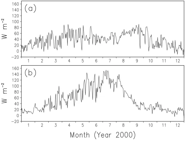
Figure 4. Year-long evolution of daily surface (a) sensible and (b) latent heat fluxes over the ARM SGP.
Figure 5. Seasonal mean diurnal variation of surface albedo from Y0 and Y1.
Figure 6. Year-long and diurnal variation of upward shortwave flux (SWUP) at the surface (SFC) from Y0 and Y1 (upper panels) based on hourly data, and the same variation of their discrepancies from observations (below panels). Figure 7. Seasonal and diurnal variations of liquid water path (LWP) and ice water path
(IWP) from Y0 and Y1, and the differences between the two simulations. Figure 8. Radiative and cloud property snapshot for three days (January 27–29, 2000)
based on hourly data.
Figure 9. Vertical profiles of potential temperature differences (a) and lapse rate differences (b) between Y0 and Y1 at 12, 16 and 21 UTC on January 27, 2000. Figure 10. Vertical profiles of domain-averaged cloud liquid and ice water mixing ratio
from Y0 and Y1 (left panels), and vertical profiles of radiative heating rate differences between Y0 and Y1 (right panels) at 16 (a) and 21 UTC (b). Figure 11. Relationship among normalized upward shortwave (SWUP) flux at the TOA,
surface albedo and CWP (i.e., LWP+IWP) (left), and the relationship with total cloud fraction (right) based on daily averaged values for the year 2000. Figure 12. Scatter diagrams of normalized upward shortwave (SWUP) flux at the TOA
versus surface albedo for all LWP ranges (a), below 50 g m-2 (b), and above 50 g m-2 (c) when solar zenith angle (SZA) is between 60° and 70°.
Figure 13. The distributions of the linear least-square-fit regression lines for the relationship between normalized upward shortwave (SWUP) flux at the TOA and surface albedo for small LWP (a), large LWP (b), small IWP (c), and large IWP (d) cases with each SZA range.
Figure 14. Scatter diagrams of normalized downward shortwave flux (SWDN) at the SFC versus surface albedo for each SZA range.
Figure 15. Scatter diagrams of surface albedo versus the cosine of SZA for each season from Y1.
Figure 16. Normalized slopes as a function of SZA for upward shortwave flux at the TOA with optically thin clouds (LWP < 50 g m-2) (a), downward shortwave flux at the SFC with optically thick clouds (CWP ≥ 180 g m-2) (b), and upward shortwave flux at the surface with all clouds (c).
Figure 17. Seasonal variation of the cloud frequency distributions as a function of the base and top heights from the CRM.
Figure 18. The non-precipitating cloud frequency distributions as a function of the base and top heights from the CRM and CPC during the year 2000.
86 87 88 89 90 91 92 94 95 96 97 98 99 100 101 102 103 104
Figure 19. Frequency distributions of all clouds as a function of month (upper panel) and diurnal variations of frequency distributions for four seasons (lower panel). Figure 20. Frequency distributions of all overcast clouds without precipitation from the
CRM and CPC as a function of month (upper panel) and diurnal variations of frequency distributions for four seasons (lower panel).
Figure 21. Frequency distributions of thick mid, low, thin high, and deep low clouds as a function of month.
Figure 22. Frequency distributions of each cloud type from the CRM and CPC as a function of month.
Figure 23. Diurnal variations of occurrence frequency distributions of thick mid, low, thin high, and deep low clouds for four seasons.
Figure 24. Diurnal variations of occurrence frequency distributions of each cloud type from the CRM and CPC for four seasons.
Figure 25. Frequency distributions of all clouds and deep low clouds as a function of month for precipitating condition.
Figure 26. Monthly averaged LWP and IWP (upper panel) from the CRM and mean diurnal variations of LWP and IWP for four seasons (lower panel).
Figure 27. Mean LWC and profiles for each bin of vertically integrated LWP from the CRM, CPC, and MICROBASE.
Figure 28. Mean IWC and profiles for each bin of vertically integrated IWP from the CRM, CPC, and MICROBASE.
Figure 29. Frequency histograms of cloud LWP and IWP for each cloud type.
Figure 30. Frequency histograms of cloud LWP and IWP for each cloud type without precipitation from the CRM and CPC.
Figure 31. Frequency histograms of cloud LWP and IWP for all clouds and deep low clouds for precipitating condition.
Figure 32. Diurnal variation of cloud optical depth calculated from the CRM for four seasons.
Figure 33. Frequency histograms of daytime cloud optical depth from the CRM and MFRSR for four seasons based on hourly mean values.
Figure 34. Frequency histograms of daytime cloud optical depth from the CRM for the entire domain, 1/2 domain, 1/4 domain, 1/8 domain, and 2 points in the CRM domain based on hourly mean values.
Figure 35. Mean vertical profiles of radiative heating rates of cloud-sky (all-sky minus clear-sky) for each cloud type from the CRM.
Figure 36. Mean vertical profiles of shortwave (SW), longwave (LW) and total cloudy radiative heating rates from the CRM and CPC for each cloud type without precipitation cases.
Figure 37. Mean vertical profiles of radiative heating rates of cloud-sky (all-sky minus clear-sky) for all clouds and deep low clouds for precipitating condition. Figure 38. An example of horizontally inhomogeneous clouds and cloud fraction profile
in the CRM domain, and the same cloud field without inhomogeneity in the D1 calculation.
Figure 39. Seasonal variation of frequency histograms for cloud inhomogeneity parameters (
χ
). 105 106 107 108 109 110 111 112 113 114 115 116 117 118 119 120 121 122 124 125 126Figure 40. Seasonal mean profiles of cloud inhomogeneity parameters (
χ
).Figure 41. Seasonal mean profiles of cloud inhomogeneity parameter (
χ
) for liquid water path (LWP).Figure 42. Seasonal mean profiles of cloud inhomogeneity parameter (
χ
) for ice water path (IWP).Figure 43. Seasonal scatter diagrams of CRM vs a diagnostic radiation calculation with homogeneous clouds (D1) for upward shortwave fluex (SWUP) at the TOA. Figure 44. Seasonal scatter diagrams of CRM vs a diagnostic radiation calculation with
homogeneous clouds (D1) for outgoing longwave radiation (OLR) at the TOA.
Figure 45. The CRM generated scatter distribution of total cloud fraction versus inhomogeneity parameter
χ
based on all 15-minute samples for the year2000.
Figure 46. Seasonal scatter diagrams of CRM vs a diagnostic radiation calculation with the parameterized reduction factor (D2) for SWUP at the TOA.
Figure 47. Seasonal scatter diagrams of CRM vs a diagnostic radiation calculation with the parameterized reduction factor (D2) for OLR at the TOA.
Figure 48. Seasonal mean profiles of shortwave, longwave and total cloud radiative heating rate differences between the CRM and each diagnostic radiation calculation (D1 and D2).
Figure 49. Scatter diagrams of total cloud fraction from the CRM versus that from the each overlap assumption (minimum, maximum and random) based on daily mean for the four seasons.
Figure 50. Schematic diagrams of cloud overlap in the CRM (or D1) and redistributed cloud fields by the three cloud overlap assumptions (maximum, minimum and random).
Figure 51. Seasonal mean profiles of shortwave, longwave and total cloud radiative heating rate differences between the D1 and diagnostic calculations (i.e., MAX, MIN and RAN).
Figure 52. Scatter diagrams of total cloud fraction based on 15-min values between the CRM and two mosaic approaches.
Figure 53. Mean radiative heating rate profiles of SW, LW and total from the original and modified (separated) mosaic approaches during the 1997 ARM IOP (26 days) over the SGP.
Figure 54. CRM simulated cloud frequency (10-2 %) distribution as a function of cloud base and top heights during the year 2000.
Figure 55. Seasonal scatter diagrams of total cloud fraction between the CRM and MOS based on 15-min samples.
Figure 56. Seasonal scatter diagrams of total cloud fraction between the CRM and MOS2 with the separation of Cs into Cs1 and Cs2 based on 15-min samples.
Figure 57. Seasonal mean vertical profiles of cloud radiative heating rates (SW, LW and Total) for MOS-CRM and MOS2-CRM.
Figure 58. Annual mean vertical profiles of radiative heating rates (SW, LW and Total) from the CRM, MOS and MOS2 for the year 2000 (a), and the annual mean profiles of MOS-CRM and MOS2-CRM (b).
127 128 129 130 131 132 133 134 135 136 137 138 139 140 141 142 143 144 145
ABSTRACT
The representation of subgrid cloud variability and its impact on radiation has been a challenge in general circulation model (GCM) simulations. To improve the representation of cloud and radiative variability and their interactions within a GCM grid, it is essential to understand subgrid cloud structures and their statistics based on long-term cloud and radiation data for various climate regions. In this study, year-long cloud-resolving model (CRM) simulations forced with the Atmospheric Radiation Measurement (ARM) large-scale forcing and prescribed evolving surface albedo were conducted for the year 2000 to document the characteristics of cloud horizontal inhomogeneity and vertical overlap and to evaluate and represent their effects on the radiative fluxes and heating rates over a GCM grid.
The year-long CRM simulations with a prescribed evolving surface albedo allow the investigation of the relationship between the surface albedo, cloud and radiation. It was found that clouds absorb more shortwave radiation at the cloud base due to a high surface albedo in winter, which increases temperature in the low troposphere. This leaded to weaker instability in the low troposphere, so that the amount of low-level clouds decreased. For surface albedo greater than a critical value of 0.35, the upward shortwave flux at the top of the atmosphere (TOA) is positively proportional to the surface albedo when optically thin clouds exist, and is not much affected by the reflection from the cloud top. If optically thick clouds occur and the surface albedo is greater than the critical value, the upward shortwave flux at the TOA is significantly affected by the reflection from of cloud top, but not much affected by the surface albedo. In addition, for a surface albedo larger than the critical value, the downward shortwave flux at the surface is primarily influenced by the surface albedo and the reflection from the cloud base if optically thick clouds occur. However, the downward shortwave flux at the surface is not much affected by the surface albedo when optically thin clouds exist because the reflection on the cloud base is weak.
The year-long cloud statistics from the CRM were evaluated against available observational data at the ARM SGP site. The CRM was able to represent thick mid-level and stratiform clouds in agreement with the observations with overcast and non-precipitating conditions. Both the CRM and observations indicated that the height of ice water content maximum in the vertical column decreases as the ice water path increases. It was found that the vertical distribution of
shortwave and longwave radiative heating rates in the troposphere were strongly affected by cloud type that was identified by cloud optical depth and vertical location. Compared to the observational estimates, the CRM-produced non-precipitating clouds had greater longwave cooling in the upper troposphere due to lower altitude of high-level clouds and greater cloud top cooling from optically thick mid-level clouds.
The ARM-validated year-long CRM simulations were used to examine the characteristics of cloud horizontal inhomogeneity and vertical overlap and to evaluate and represent their effects on the domain mean radiative flux and heating rate. The analysis of an inhomogeneity parameter (or reduction factor) defined as a ratio of the logarithmic and linear averages of cloud liquid and ice water paths demonstrated that inhomogeneous clouds more frequently appear in summer than in winter due to the occurrence of different cloud types dominated between two seasons. A parameterization with the reduction factor derived from the year-long CRM simulation captured the dominant impact of cloud inhomogeneity on the shortwave and longwave radiative flux and heating rate. Diagnostic radiation calculations with three overlap assumptions (i.e., maximum, minimum, and random) indicated large biases in the total cloud fractions, domain mean shortwave and longwave radiative fluxes, and radiative heating rates when compared to the CRM simulations. These results suggest the need for a physically-based parameterization that treats the differences of characteristic structure between major cloud types such as convective, anvil and stratiform clouds in order to account the radiative effects of subgrid cloud variability on the domain means.
The original mosaic treatment was developed by modifying a GCM radiation scheme to incorporate the radiative effects of dominant cloud types including convective, anvil and stratiform clouds. It cannot be readily used for different radiation schemes. In this study, a cloud distribution scheme was formulated outside of the radiative transfer scheme, so that it can be applied to any GCM to include the radiative effects of cloud variability in their radiative transfer calculations. The radiation calculation with the cloud distribution scheme improved by the year-long CRM statistics produced domain mean shortwave and year-longwave radiative fluxes and heating rates comparable to the CRM values in seasonal and annual means, which indicates the cloud distribution scheme represents cloud variability in the much the same way as the CRM does.
CHAPTER 1. INTRODUCTION
Cloud systems play an essential role in general circulation models (GCMs) through their direct and indirect feedbacks with atmospheric radiation. Radiative fluxes and heating rates are calculated on discrete grid columns using grid-mean values with radiative transfer schemes. However, the GCMs cannot accurately represent the effect of clouds on radiative transfer energy in the atmosphere (interaction between clouds and atmospheric radiation) because of their coarse horizontal resolution of several hundred km spacing. In order to approximate the effect of the subgrid spatial and temporal variability of clouds, there has been much effort to incorporate the effect into large-scale model simulations using numerous parameterization schemes (e.g., Cess et al. 1989; Browning 1994; Fowler et al. 1996; Jabouille et al. 1996; Barker and Räisänen 2005;
Räisänen et al. 2007). The radiation parameterizations are very sensitive to the spatial and temporal distribution of cloud systems (Webster and Stephens 1984; Ramanathan et al. 1989; Kiehl et al. 1994). Especially, the horizontal and vertical distributions of clouds and their microphysical properties strongly affect the radiative energy budgets in those models (Manabe and Strickler 1964; Geleyn and Hollingsworth 1979; Stephens 1984; Cahalan et al. 1994; Liang and Wang 1997; Morcrette and Jakob 2000; Li et al. 2005; Barker and Räisänen 2005; Tompkins and Giuseppe 2007; Gustafson et al. 2007). In most current large-scale models some overlap assumptions are applied to instantaneous profiles of domain-averaged cloud properties to infer subgrid-scale structure. These cloud properties include the portion of each grid box occupied by cloud (i.e., cloud fraction) and the mean liquid and ice condensate. The large-scale models have typically used one of three simple assumptions: random, maximum and maximum-random (Geleyn and Hollingsworth 1979; Liang and Wang 1997; Morcrette and Jakob 2000; Collins 2001; Stephens et al. 2004). Since these cloud vertical overlap assumptions can predict only the mean value of cloud properties in each model grid, the models are subject to significantly large biases in convective and radiative processes. The biases caused by unresolved subgrid-scale inhomogeneity appear to be one of the major reasons that GCMs need to be tuned. Therefore, GCMs do not explicitly specify vertical geometric associations and horizontal inhomogeneity of clouds. As a result, the effects of vertical overlap and horizontal inhomogeneity of clouds are not properly represented in GCMs yet since most cloud overlap methods in large-scale models are not physically consistent or are empirical without rigorous evaluation, and some methods
produce intolerable errors in calculating grid-mean fluxes (Stephens et al. 2004). Furthermore, recently obtained long-term radar records indicate that clouds are less vertically coherent than the maximum-random assumption implies. These observations suggest that cloud occurrence within vertically continuous cloud layers decays inverse-exponentially from maximum to random overlap as the vertical distance separating cloud layers increases, with a scale length of several kilometers (Hogan and Illingworth 2000; Mace and Benson-Troth 2002). These studies suggest that only the single cloud overlap assumption cannot be properly applied in a large-scale model. This may mean that the cloud overlap should be parameterized using statistics of synoptic-scale characteristics that describe the cloud formation. The parameterization of cloud vertical and horizontal distribution in GCMs is still a key issue because of the lack of available observations for assessing the parameterization in the models and the lack of comprehensive understanding of the effects of cloud systems and their feedback with convective and radiative processes that may offer information on the effects of subgrid cloud variability and corresponding cloud-radiation interaction.
Cloud-resolving models (CRMs) have been recognized as a powerful tool to examine cloud systems over various different climate regions and under various large-scale conditions. CRMs could represent a reasonably realistic ensemble of clouds and statistical properties of cloud systems with large-scale vertical velocity or the large-scale horizontal and vertical advection, and have also been used to investigate convective systems, cloud properties and their radiative effects (e.g., Soong and Ogura 1980; Soong and Tao 1980; Krueger 1988; Xu et al. 1992; Wu and Moncrieff 1996; Grabowski et al. 1996; Wu et al. 1998, 1999, 2007; Wu and Moncrieff 2001). The CRM simulations have been assessed with various observations in terms of atmospheric thermodynamic properties, atmospheric radiation, precipitation, and surface fluxes in the tropics during the Global Atmospheric Research Program Atlantic Tropical Experiment (GATE) (e.g., Xu and Randall 1996; Grabowski et al. 1996), Tropical Ocean Global Atmosphere Coupled Ocean Atmosphere Response Experiment (TOGA COARE) (e.g., Wu et al. 1998; Li et al. 1999; Wu and Moncrieff 2001), and ARM (e.g., Xu et al. 2002; Wu et al. 2007, 2008).
Grabowski et al. (1996, 1998, 1999) conducted 2-dimensional (2D) and 3-dimensional (3D) CRM simulations with evolving large-scale forcing and evolving horizontal wind fields during phase III of GATE and showed that various types of clouds can be well represented by the CRM, and that low-resolution 2D CRM can be used in the climate problem and for improving and
testing cloud parameterization for GCMs. They also investigated the effects of cloud microphysics on the convective tropical atmosphere by performing several numerical experiments with extreme changes in cloud microphysics. Another 2D CRM simulation was performed during TOGA COARE to quantify the collective effects of cloud systems, to improve the simulation of cloud fields through demonstrating the effects of ice phase processes on cloud-radiation interaction, and to examine the effects of cloud systems on radiative energy budgets at the surface and top of the atmosphere (TOA) (Wu et al. 1998, 1999; Wu and Moncrieff 2001). Wu and Moncrieff (2001) showed that CRM-simulated energy budgets are in good agreement with observations, while the corresponding quantities derived from a single-column model (SCM) have large biases during TOGA COARE. They also explained that the CRM is able to represent cumulus convection explicitly, including its mesoscale organization, and produce vertical and horizontal distributions of cloud condensate that interact much more realistically with radiation than those in the SCM. The CRM simulation is also used to investigate the vertical transport of horizontal momentum and the role of a convection-generated perturbation pressure field (Zhang and Wu 2003). Tao et al. (2004) simulated a 2D CRM to examine the atmospheric energy budget and large-scale precipitation efficiency of various convective systems in east Atlantic, west Pacific, South China Sea, and SGP and found that for the cloud systems developed over a midlatitude continent, the net radiative and surface heat fluxes play a much more important role than those in tropics. Wu and Liang (2005) quantitatively revealed the horizontal inhomogeneity and vertical overlap effects of clouds on radiative fluxes over a 30-day period during TOGA COARE conducting a CRM simulation and found that both horizontal and vertical distribution effects of clouds are equivalently important to obtain more realistic radiative fluxes and heating rates. They also suggested an objective procedure to evaluate the parameterization for subgrid cloud-radiation interactions in a GCM using the CRM simulation. Xie et al. (2005) found that SCMs usually have very significant biases due to the lack of subgrid-scale dynamical structure and organized mesoscale hydrometeor advections while the CRM-simulated cloud properties are very comparable with observations, through evaluating nine SCM and four CRM simulations during the spring 2000 ARM IOP at the SGP site. Wu and Guimond (2006) conducted 2D and 3D CRM simulations to quantify the enhancement of surface heat fluxes by tropical precipitating cloud systems for 20 days during TOGA COARE and suggested that subgrid processes (e.g., the mesoscale enhancement of surface heat fluxes) is imperative to incorporate into GCMs.
Blossey et al. (2007) compared the simulated cloud properties from a 3D CRM with observations over Kwajalein Experiment (KWAJEX) and tested the model’s sensitivities on microphysics, radiation scheme, effective radii, surface forcing, and domain and grid size of the model. They showed that the amount and optical depth of high cloud are underpredicted by the model during less rainy periods, leading to excessive outgoing longwave radiation, and the simulated high clouds are precipitating large hydrometeors too efficiently. Ping et al. (2007) performed three 2D CRM simulations to investigate the microphysical and radiative effects of ice clouds on tropical equilibrium states and found that the ice radiative effects on thermodynamic equilibrium states are stronger than the ice microphysical effects. Wu et al. (2007) simulated a CRM for the 1997 ARM IOP over SGP site to provide physically consistent long-term data together with observations, which facilitates quantifying the effects of subgrid cloud-radiation interactions in GCMs. They also compared the cloud systems in TOGA COARE and those in ARM SGP and then showed that the CRM-produced cloud distributions in the two different regions are very different because of the different large-scale forcing and surface heat fluxes, but the subgrid cloud variability has similar effect on radiative fluxes and heating rates in the tropics and midlatitude continent. Recently, the convection and cloud parameterization schemes in GCMs have been replaced by CRMs to explicitly simulate the interaction among convection, clouds, radiation and large-scale circulation (e.g., Grabowski 2001, 2004; Randall et al. 2003; Khairoutdinov et al. 2005; Wyant et al. 2006). Also, as a global CRM, a Nonhydrostatic Icosahedral Atmospheric Model (NICAM) has been developed to investigate cloud-scale phenomena explicitly interacting with large-scale circulation such as monsoon-related convective activity and Madden-Julian Oscillation (Tomita and Satoh 2004; Tomita et al. 2005; Miura et al. 2005, 2007; Sato et al. 2007).
The previous CRM studies were limited in their simulating time, for instance only a few days, weeks or months. The products from the shortly integrated simulations cannot necessarily generalize the clouds’ characteristics and their interaction with atmospheric radiation in various climate regions. In fact, the available large-scale forcing data were limited only in several short field experiments such as GATE, TOGA CORAE and ARM IOPs to simulate CRMs long enough to consider general characteristics of clouds. Recently, the ARM program has been producing long-term cloud macroscopic properties (e.g., cloud top and base height and fraction) and microphysical properties (e.g., liquid and ice content) of clouds and corresponding radiative
fluxes using active and passive remote sensing instruments at the ground and from satellites. For example, a long-term (8 years) cloud data set including atmospheric thermodynamic, cloud and radiative properties for the ARM SGP site were produced by Mace et al. (2006) and Mace and Benson (2008) using the column physical characterization (CPC) technique. The CPC data set contains various macroscopic and microphysical cloud properties such as the height, pressure and temperature of cloud base and top, cloud fraction profile, visible optical depth, cloud thickness, and cloud liquid and ice water content. Another data set, MICROBASE (Miller et al. 2003) data over the ARM SGP, is also available from the ARM website. This data set was retrieved by a combination of observations from a millimeter cloud radar (MMCR), laser ceilometer, micropulse lidar (MPL), the microwave radiometer (MWR) and a merged thermodynamic profile to estimate the profiles of liquid and ice water content, cloud fraction and effective radius of cloud particles. Moreover, multi-year forcing data over the ARM SGP site were constructed using the mesoscale analysis and the ARM measurements at the ground and from satellites (Xie et al. 2004). This longer large-scale forcing data allow the longer integration of CRMs to provide generalized seasonal characteristics of clouds and their interaction with radiative properties.
Recently, Wu et al (2008) conducted a year-long Iowa State University (ISU) CRM simulation using the large-scale forcing over ARM SGP during year 2000 to investigate the seasonal variation of radiative and cloud properties. The year-long simulation provides a physically consistent long-term dataset for understanding the processes of convection, cloud and radiation and the interaction among them. However, large discrepancies of net shortwave (SW) flux between the CRM and observations at the surface were presented in winter time due to the use of fixed surface albedo. If realistically evolving surface albedo is used in the CRM, the discrepancies could be reduced, and also the more realistic long-term CRM dataset could be used to quantify seasonal and spatial characteristics of cloud systems over the ARM SGP.
Therefore, the hypotheses in this dissertation are as follows. First, seasonal and spatial variations of cloud systems over the central US can be simulated and quantified by the CRM integration. Second, long-term CRM simulations could provide a robust cloud-scale data for investigating the cloud ensemble effects and their relationship with the large-scale conditions. Third, subgrid cloud distributions and their radiative effects can be represented by the mosaic approach for the application in GCMs. In the next chapter, the ISUCRM and large-scale forcing
data are introduced. In chapter 3, the effects of surface albedo on cloud and radiative properties are investigated using the year-long CRM simulation with the prescribed evolving surface albedo. In chapter 4, statistical analysis of year-long cloud and radiative properties is performed to characterize cloud types and their impacts on radiation. In chapter 5, subgrid cloud variability in the CRM is examined in terms of cloud horizontal and vertical distributions. Chapter 6 shows the mosaic approach for subgrid cloud distribution and evaluation with the year-long CRM simulations. General conclusion is given in chapter 7.
CHAPTER 2. METHODOLOGY
1. ISU Cloud-Resolving Model
The ISUCRM used in this study is originally from the 2D version of the Clark-Hall anelastic cloud model (Clark et al. 1996) that has the imposed large-scale forcing and the modified physical processes significant for the long-term simulations of cloud systems (Grabowski et al. 1996; Wu et al. 1998, 1999, 2007; Wu and Moncrieff 2001). The Kessler (1969) bulk warm rain parameterization and the Koenig and Murray (1976) bulk ice parameterization are adopted in the microphysical processes of the model. The ice parameterization products two types of ice particles; type-A ice represents slowly falling and low-density ice such as unrimed or slightly rimed particles, and type-B ice is relatively fast-falling and high-density ice such as graupel. Each type of ice is represented by two variables (i.e., mixing ratio and number concentration). For the radiative transfer calculation, the radiation scheme of the NCAR Community Climate Model (CCM) (Kiehl et al. 1996) is imposed with the use of binary liquid and type-A ice clouds which have effective radii of 10 and 30 ㎛, respectively. The first-order eddy diffusion method of Smagorinsky (1963) is also applied to parameterize the subgrid-scale mixing. Periodic lateral boundary conditions are adopted to facilitate a mathematically consistent CRM framework (Grabowski et al. 1996). Free-slip, rigid bottom and top boundary conditions are applied with a gravity wave absorber between 16 km and the model top. In order to distribute the surface heat fluxes, a nonlocal vertical diffusion scheme (Troen and Mahrt 1986; Holtslag and Moeng 1991; Hong and Pan 1996) is used within the boundary layer. The ISUCRM uses a 2D east-west 600 km horizontal and 40km vertical domain. The horizontal grid size is 3 km and the vertical grid of 52 levels is 100 m at the surface, 550-850 m between 5 and 12 km, and 1500 m at the model top. The simulation time step is 15 s. The model setting of the year-long (i.e., January 3-December 31, 2000) CRM simulation is basically the same as the CRM simulation by Wu et al. (2008). The year-long CRM simulation is forced by the evolving temperature and moisture forcing which is kept constant for an hour around the observed time. The domain-averaged wind at each time step is relaxed using a 2-hour time scale to the observed wind. The CRM uses the prescribed evolving surface sensible and latent heat fluxes from observations. The observed wind and surface heat fluxes are interpolated into each model time step. The observed
evolving surface temperature is used to calculate the surface upward longwave radiative flux. Originally, the surface albedo for direct and diffuse incident solar radiation is set to 0.05 and 0.25 for two spectral intervals, 0.2-0.7 µm and 0.7-0.5 µm, respectively. The constant surface albedo is replaced with the prescribed evolving surface albedo for new CRM simulation in the next chapter. Hereafter, the CRM simulation by Wu et al. (2008) is referred to as Y0 and the new one is referred to as Y1. The radiative fluxes and heating rate are computed every 300 s and applied at intermediate times. Random perturbations are added to the temperature (0.1 K) and moisture (0.1 g kg-1) fields across the 2D domain (vanishing when averaged over the domain) within the boundary layer every 15 m for the convection initiation.
2. Large-scale forcing data
The year-long hourly large-scale forcing data were constructed using the variational analysis of NWP model-produced fields constrained by surface and TOA observations over the ARM SGP site including precipitation, latent and sensible heat fluxes and radiative fluxes (Xie et al. 2004). The time evolution of vertically-integrated daily temperature and moisture forcing over the ARM SGP site during the year 2000 is shown in Fig. 1. There is an obvious seasonal variation of temperature forcing with stronger advective cooling (negative values in Fig.1a) in summer and spring, and weaker advective cooling in winter and fall. The stronger advective cooling is generally correspondent with the stronger advective moistening (positive values in Fig.1b). Figure 2 further presents the seasonal variation of the vertical distribution of temperature and moisture forcing. Large cooling is located between 4 and 10 km with a peak around 7 km in summer and spring, while the cooling is smaller in autumn with virtually no tropospheric cooling in winter (Fig.2a). Advective moistening exists above 1 km in spring, autumn and winter but above 2 km in summer (Fig.2b). The large advective drying below 2 km in summer is largely due to the drying occurring during August. Winter has the smallest moistening while other seasons have the peaks of moistening at different levels (3, 4 and 5 km for autumn, summer and spring, respectively).
Figure 3 presents the seasonally-averaged zonal and meridional components of horizontal wind. Through the four seasons, westerly wind is dominant with peaks around 11 and 12 km (Fig.3a). Winter has the strongest vertical wind shear (35 m s-1 over 12 km), while summer has the weakest shear (10 m s-1 over 12 km). The profiles of meridional wind (Fig.3b) indicate
southerly peaks around 0.5 and 0.8 km through four seasons. Northerly wind prevails in winter, while the southerly is dominant in autumn. The strongest vertical shear of meridional wind occurs between 1 and 4 km in summer. Figure 4 illustrates the year-long evolution of daily observed surface sensible and latent heat fluxes. Winter has the smallest sensible and latent fluxes of about 20 W m-2. In summer, latent fluxes have the maximum with a mean of 104 W m
-2
CHAPTER 3. EFFECTS OF SURFACE ALBEDO
1. Introduction
Surface albedo plays an essential role in determining the energy budget at the surface and the top of the atmosphere (TOA). Most albedo-related studies have focused on snow-albedo feedback and its impacts on climate sensitivity in general circulation model (GCM) simulations (Schneider and Dickinson 1974; Randall et al. 1994; Hall 2004; Winton 2006; Qu and Hall 2007). In addition, studies have been conducted over the high latitude regions such as Alaska, Greenland and the other Arctic and Antarctic regions in order to examine the effects of surface albedo and clouds on ultraviolet (UV) radiation through comparing snow-covered and snow-free area and to quantify its temporal and spatial characteristics (Baker and Ruschy 1989; Stamnes et al. 1990; McKenzie et al. 1998; Kylling et al. 2000). For instance, Huber et al. (2004) quantified the effect of horizontal inhomogeneity of surface albedo on diffuse UV radiation at High Alpine Research Station in Jungfraujoch, Switzerland using a discrete ordinate radiative transfer model. There have also been some studies on the desert albedo using satellite data. Tsvetsinskaya et al. (2002) reported that satellite data have convincingly shown the considerable spatial variation of desert albedo by analyzing the Moderate Resolution Imaging Spectroradiometer (MODIS) retrievals. Wang et al. (2005) also found bare soil albedo is not only a function of soil color and moisture, but also solar zenith angle (SZA) using the MODIS Bidirectional Reflectance Distribution Function (BRDF) and albedo data over thirty desert regions.
Those previous studies have usually more focused on the effects on UV radiation rather than the relationship between surface albedo and clouds. Nichol et al. (2003), however, showed that a great amount of surface albedo can moderate the attenuation of UV radiation by cloud through the multiple scattering between the cloud base and the surface in the high latitudes. Shupe and Intrieri (2004) also examined the relationship between surface albedo and cloud radiative forcing over an Arctic region using the cloud and radiation dataset from the Surface Heat Budget of the Arctic (SHEBA) program. For middle latitude cases, some research groups have investigated various surface albedo-related phenomena. Grant et al. (2000) examined the dependence of clear-sky albedo on SZA by observing daily variation of surface albedo at Uardry in southeastern Australia. Considering the impact of observed surface albedo over the Department of Energy’s Atmospheric Radiation Measurement Program (ARM) Southern Great Plains (SGP) during two
winter seasons, Dong (2005) improved a parameterization for low-level cloud properties. The parameterization was able to represent the effect of surface albedo on the stratus cloud microphysical and radiative properties. Duchon and Hamm (2006), analyzing observed daily broad band surface albedo over the ARM SGP for two years (1998 and 1999), reported that there is obvious horizontal inhomogeneity of surface albedo among the six observational ground stations, and surface albedo over bare soil is significantly affected by precipitation but vegetated surfaces are not strongly affected. They also found that on an overcast day surface albedo tends to decrease. Yang et al. (2006) used direct and diffuse surface albedo produced from ARM SGP and Tropical Western Pacific (TWP) sites during 1997-2004 to evaluate the parameterization of the dependence of surface albedo on SZA used by the National Centers for Environmental Prediction (NCEP) Global Forecast Systems (GFS) and those derived by a satellite observation. Recently, Yang et al. (2008) showed the dependence of snow-free surface albedo on SZA using the surface albedo data obtained from nine measurement stations whose surface types and locations are very different from each other during 1997-2005.
Recently, a year-long CRM simulation was conducted over ARM SGP during the year 2000 by Wu et al. (2008) to investigate the seasonal variation of radiative and cloud properties. The year-long simulation provides a physically consistent long-term dataset for understanding the processes of convection, cloud and radiation and the interaction among them. However, large discrepancy of net shortwave (SW) flux between the CRM and observation at the surface is present in winter time due to the use of fixed surface albedo.
The relationship between the surface albedo, radiative fluxes and cloud properties cannot be investigated with the CRM using the fixed surface albedo. If the surface albedo in the CRM is varied diurnally and seasonally, the relationship would be revealed. In this study, a year-long simulation is performed over the ARM SGP site during the year 2000 using the Iowa State University (ISU) CRM with the prescribed evolving surface albedo from the ARM observational estimates. The objectives of this chapter are 1) to examine the effects of the evolving surface albedo on the CRM simulation and 2) to investigate the relationship between the surface albedo, cloud properties and radiative fluxes.
2. Prescribed evolving surface albedo
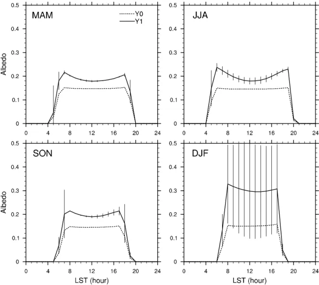
albedo is calculated as the ratio of upward SW flux to downward SW flux at the surface. Since the CRM uses surface albedos of direct and diffuse incident radiation for two spectral intervals in radiative transfer calculation, the broadband surface albedo (AB) is decomposed into two parts for wavelength 0.2-0.7 micrometers (AS) and 0.7-5.0 micrometers (AL), respectively. When AB is equal to or smaller than 0.21 the ratios of AS/AB and AL/AB are set to 0.19 and 0.81, respectively (Briegleb 1992). When AB is equal to 1.0, AB is equally divided between AS and AL so that, in the albedo range from 0.21 to 1.0, AS/AB and AL/AB are linearly increased and decreased, respectively, until AB = 1.0. The separation of surface albedo into AS and AL might be inappropriate in certain conditions, since the surface albedo has strong dependence on solar zenith angle, soil type, soil moisture and vegetation type (Liang et al. 2005). The prescribed surface albedo is imposed in the computation of radiative fluxes and heating rates every 300 seconds. The difference of surface albedo between the two CRM runs is showed in Fig. 5 in terms of seasonal change of diurnal variation. The albedo of Y0 (Wu et al. 2008) is almost constant as 0.15 during daytime throughout four seasons, while that of Y1 has distinct diurnal variation and also has relatively much greater values in the winter. The surface albedo differences between Y0 and Y1 are about 0.05 in the spring, summer and fall and 0.15 in the winter, respectively. Because of snow-covered periods, the standard deviations in winter are relatively larger than the other seasons. Usually the early morning and late afternoon albedo is greater than the other period during the daytime, and the early morning albedo is slightly greater than late afternoon albedo. This asymmetry is mainly caused by the direct beam albedo (Yang et al. 2008), and is possibly due to the dew effect in the early morning (Minnis et al. 1997).
3. CRM-simulated radiative and cloud properties
The general characteristics of radiative fluxes and cloud properties from the CRM were shown by Wu et al. (2008) with the constant surface albedo. In this section, the major effects of the prescribed evolving surface albedo on radiative and cloud properties are shown in the annual and seasonal aspects.
The annual and seasonal means and standard deviations of net longwave (LW) and SW radiative fluxes at TOA and the surface from Y1 and observations are listed in Table 1. The net flux is defined as the downward minus upward fluxes. The observed TOA LW and SW fluxes are derived from GOES (Minnis et al. 1995). The CRM-produced annual mean LW is close to the
observed LW at TOA with the difference of less than 1 W m-2 and at the surface with the difference of less than 6 W m-2. For the seasonal means, the differences of LW between Y1 and observations are within 7 W m-2 at TOA and within 11 W m-2 at the surface. The differences of the annual mean SW flux between Y1 and observations are less than 8 W m-2 at TOA and the surface. The use of prescribed surface albedo in Y1 makes winter time SW flux be much more comparable with observations. The difference from the observations is about 3 W m-2 at the surface in winter. However, the discrepancies of SW radiative budgets of annual and the other seasons between the CRM and observations are not negligible. The uncertainty in obtaining the area mean surface SW flux from 22 stations may be partly responsible for those discrepancies (Li et al. 2002). The albedo difference in winter is important because there are many low level clouds over ARM SGP in the winter of the year 2000 (Wu et al. 2008). Table 2 lists annual and seasonal means and standard deviation of upward and downward fluxes of SW and LW based on daily averaged values. At the surface, downward and upward LW budgets are very similar between Y1 and observations with the differences of less than 2 W m-2 throughout the whole year, and upward SW flux budgets of Y1 are also very close to the observations due to the use of prescribed evolving surface albedo. However, the differences of downward SW flux between Y1 and observations are large at the surface. Especially, upward SW fluxes at the surface from Y1 are close to observations. Annual means of Y1 and observation are 42.2 and 40.5 W m-2, and winter means are 35.3 and 32.4 W m-2, respectively. Since the solar insolation at TOA and the surface are usually much greater in summer than the other seasons, despite the relatively small albedo difference of 0.05 between Y0 and Y1, the corresponding effect on SW flux is very large. For example, the summer mean solar insolation is 458 W m-2 and the winter mean is 214 W m-2 at TOA, and the mean surface albedo differences are 0.05 and 0.15 in summer and winter. However, the corresponding differences in net SW flux are about 10 W m-2 and 12 W m-2 in summer and winter, respectively. Therefore, surface albedo effect on SW radiative budget depends on the intensity of solar insolation at TOA through the entire year.
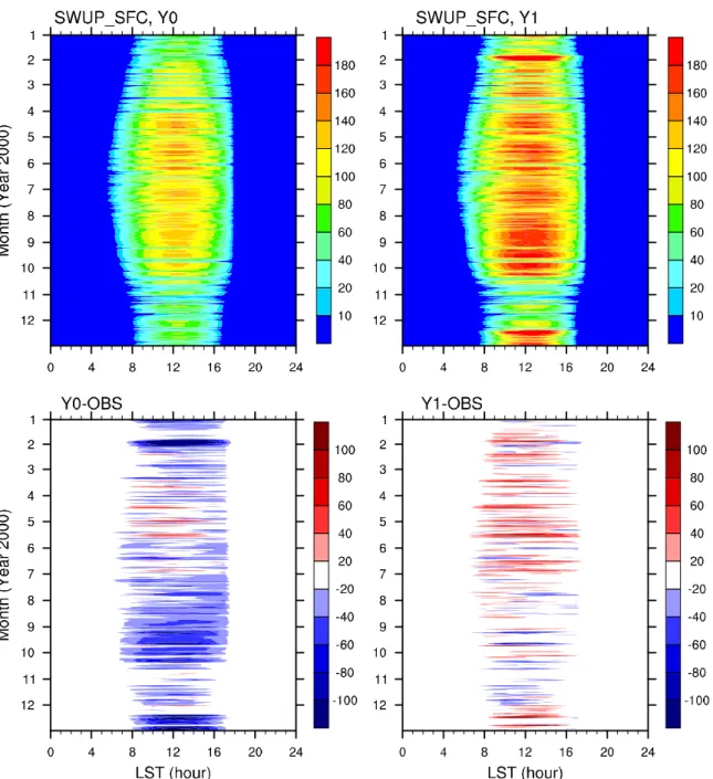
The primary difference in radiative flux between Y1 and Y0 is revealed in upward shortwave (SWUP) flux at the surface as shown in Fig. 6. This figure indicates the daily variation of SWUP from Y0 and Y1 at the surface and differences from observations. Since the surface albedo of Y1 is usually greater than that of Y0, the SWUP of Y1 is generally greater than that of Y0 throughout the entire year. Especially, the winter values of Y1 are much larger when
snow-cover exists on the SGP site. The differences between Y0 and observations are usually large; the SWUP from Y0 is much smaller than that from observations in January, February, September and December. The SWUP of Y1 is much improved during those periods.
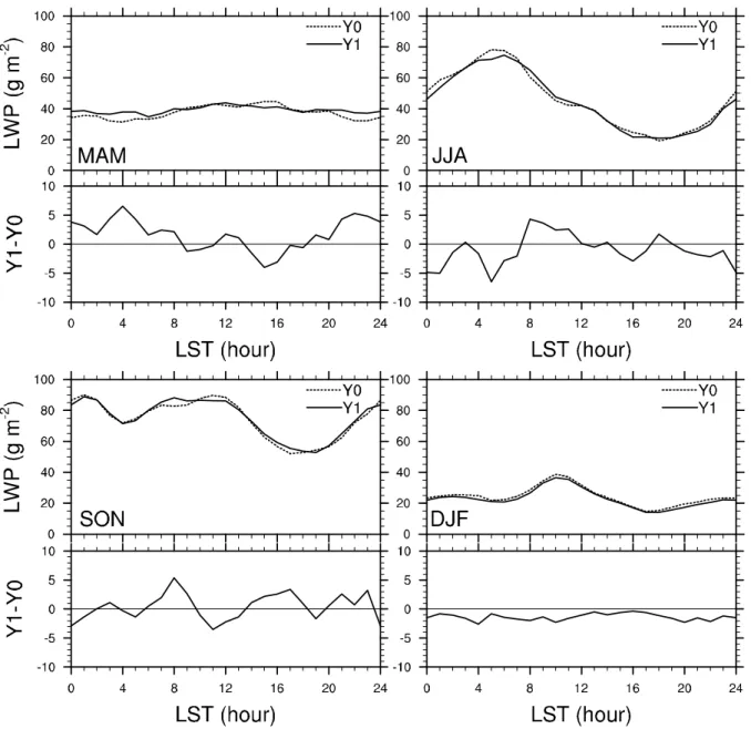
Comparison Y1 with Y0 in terms of cloud properties such as liquid water path (LWP) and ice water path (IWP) gives insight to the effect of surface albedo difference on cloud fields. The albedo effect on cloud systems might be an indirect process by which convection and temperature and moisture field could be varied after the change of radiative fluxes. Because of the prescribed surface heat fluxes, the surface albedo effects on cloud systems could be underestimated in this study. Figure 7 shows seasonally averaged diurnal variation of vertically integrated LWP and IWP from Y0 and Y1 based on hourly averaged values. The differences between the two simulations are also showed. In the spring, Y1 has usually a greater amount of clouds at night, for instance 20-5 local standard time (LST), about 5 g m-2 and 20 g m-2 more in LWP and IWP respectively, while Y1 has fewer clouds just before sunset, but daytime cloud amounts of Y1 are comparable with Y0. However, in the summer, Y1 has usually fewer clouds during the nighttime (19-3 LST, about 5 g m-2 and 10 g m-2 less in LWP and IWP respectively) and greater clouds in the morning (7-11 LST). Y1 also has slightly greater clouds before sunset in the summer. In the fall, Y1 cloud systems tend to have larger LWP (3 g m-2 more) and IWP (5 g m-2 more) than Y0 in the evening (15-23 LST). Through the entire day, Y1 clouds have about 2 g m-2 lesser LWP in the winter, but the amount of IWP of Y1 is almost comparable to Y0 except 3, 20 and 22 LST. The discrepancy between Y0 and Y1 in the winter is primarily caused by the great difference (0.15) in surface albedo between the two runs, which will be discussed in the next section.
4. Surface albedo effects
In addition to the annual and seasonal analyses of the year-long ISUCRM simulation with the prescribed evolving surface albedo in radiative fluxes and cloud properties, further analyzing the production from the CRM allows the quantification of effects of surface albedo on radiative fluxes and cloud properties.
a. Surface albedo effects on cloud properties and radiative fluxes
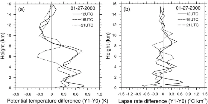
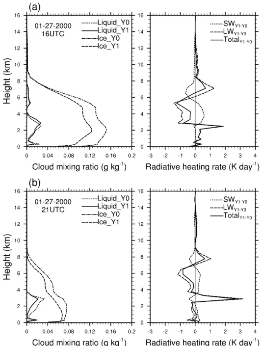
time. From the CRM simulation, only 7 days are found as meaningful cases with large clouds (i.e., the sum of LWP and IWP is greater than 100 g m-2) and great surface albedos (i.e., greater than 0.4) in the winter of the year 2000. However, most cases (6 cases) have their major events in the night and only one case occurs in daytime. From the case study during the daytime, the relationship among the surface albedo, radiative fluxes and cloud properties can be investigated when surface albedo is very high and cloud amount is very large. Figure 8 shows the case during 27-29 January, 2000 based on hourly mean values. Downward SW flux at TOA (i.e., solar insolation) and upward longwave (LWUP) flux at the surface from Y1 must be same as those from Y0, because incoming solar radiation should be equivalent and the prescribed surface heat fluxes are same in the two simulations. During this period, surface albedo of Y1 is much greater than that of Y0 because the surface is covered by snow, and the difference of surface albedo between the two simulations is about 0.6. At TOA, the SWUP of Y1 should be larger than that of Y0 as 28th and 29th cases due to the surface albedo differences. However, the SWUP fluxes at TOA on 27th from both simulations are almost equivalent each other in spite of the great surface albedo difference. That is primarily caused by the occurrence of clouds (Figs. 8h and i) reflecting SW flux from the cloud top. The SWDN fluxes at the surface are smaller on the 27th because of absorption by clouds, while the fluxes on the other days are large in the two simulations, as expected. However, SWUP at the surface from Y1 is much larger than that from Y0 due to the great reflection from the surface. Considering Figs. 8d, e, h and i, it is noticed that SWDN at the surface can be affected by the cloud bottom reflection of SW flux coming from the surface. Therefore, the SW radiative flux is affected by surface albedo together with cloud through the reflection on cloud top and base. Besides in terms of LW flux (Figs. 8c and f), LWUP at TOA and LWDN at the surface are also different between the two simulations when clouds exist (Figs. 8h and i).
Since we are interested in the surface albedo effect on clouds, only daytime (i.e., 13-23 UTC) variations of the surface albedo and cloud properties are considered. During the daytime on 27th, IWP and LWP of Y1 are usually smaller than those of Y0 (the large IWP and LWP of Y1 in the early morning, before sunrise, will be discussed later). Unlike the variation of LWP in Y0, that of Y1 is dramatically decreased from the morning to late afternoon. The possible reason is that because of greater surface albedo in Y1 simulation, the heating of the lower troposphere is increased due to additional absorption of SW radiation by water vapor and clouds, so that
temperature is increased (Fig. 9a). During the daytime (16 and 21 UTC), the potential temperature of Y1 is larger than Y0 in the lower troposphere. The change of temperature profile leads to the change of temperature lapse rate. Figure 9b shows the vertical profiles of lapse rate (i.e., dT/dz) differences between the two simulations at 12, 16 and 21 UTC. During the daytime (16 and 21 UTC), the lapse rates in the lower troposphere are much smaller (-0.3 and -0.7 oC km
-1
) in Y1, which leads to fewer clouds in Y1 simulation. Figure 10 illustrates the vertical profiles of cloud liquid and ice mixing ratios at two points in the daytime. The cloud graupel and rain water mixing ratios are very small in this period. The amount of ice clouds is much fewer in Y1 and liquid clouds of Y1 are also decreased from 16 to 21 UTC. The great amounts of IWP and LWP in the early morning could be explained by the greater lapse rate (+0.9 oC km-1) in the lower troposphere before sunrise (Fig. 9, 12 UTC). Since Y1 has fewer liquid and ice cloud particles during most of the daytime, the corresponding changes of radiative heating rates are also similar between at 16 and 21 UTC (Fig. 10). There are less LW radiative cooling around cloud top, more cooling inside clouds and more cloud base heating due to the weaker blocking of LW flux from the surface, while there are more SW radiative cooling due to the less reflection on the cloud top and more heating inside clouds because of more incoming SW radiation. Thus, the large surface albedo induced less clouds result in net radiative heating in the upper and lower troposphere and net radiative cooling in the middle troposphere in winter. Because of the fewer clouds during the daytime, the LWUP from the surface is less blocked by the clouds thereby slightly increasing LWUP at TOA. The fewer clouds cause less LWDN from the cloud base and then LWDN at the surface is decreased. As shown in Fig. 8, 9 and 10, surface albedo affects not only SW flux budget, but also cloud systems via influencing temperature and instability in the lower troposphere, thereby affecting LW flux as well. However, the surface albedo effect on cloud properties cannot be generalized with one case study. Usually in other cases in winter, the effect on clouds is small.
Cloud radiative forcing (CF) on SW and LW fluxes could be used to examine those processes among cloud, radiative fluxes and surface albedo. Especially, the shortwave and longwave cloud radiative forcing (SWCF and LWCF, respectively) could generally be used as a measure of the large-scale effects of clouds on radiative fluxes. The cloud radiative forcing is defined as the difference between the net radiative flux of all sky and the net radiative flux corresponding to clear-sky conditions. As shown in Table 3, seasonal mean values of SWCF and
LWCF are obtained at TOA and the surface from Y0 and Y1 simulations, respectively. The annual and seasonal mean values of CF from the two simulations averaged over 600 km domain are listed. The annual and seasonal characteristics of CF from Y0 are well discussed by Wu et al. (2008). In terms of annual mean, the two simulations are almost equivalent to each other in LWCF, while there are significant differences (e.g., 4 W m-2 and 5 W m-2 at TOA and the surface, respectively) between the simulations in SWCF. The discrepancies of SWCF between Y0 and Y1 are 2-4 W m-2 in the spring, summer and fall at TOA and the surface. However, the difference is significantly great during the winter time by 7-8 W m-2, primarily due to the different surface albedo. Moreover in the seasonal aspect, the LWCFs from the two simulations are almost same during MAM, JJA and SON, while the difference of winter LWCF at the surface between two simulations is much greater by 13 W m-2, which might be caused by the frequently occurring low-level clouds over the ARM SGP in winter. In order to explicitly show the process between the surface albedo and near surface clouds, surface temperature and surface heat fluxes need to be physically interacted with surface albedo. Some implicit impacts are shown in this frame work, but to tease out more realistic feedback of surface albedo to radiation and clouds, the CRM need to be improved in treatment of surface conditions.
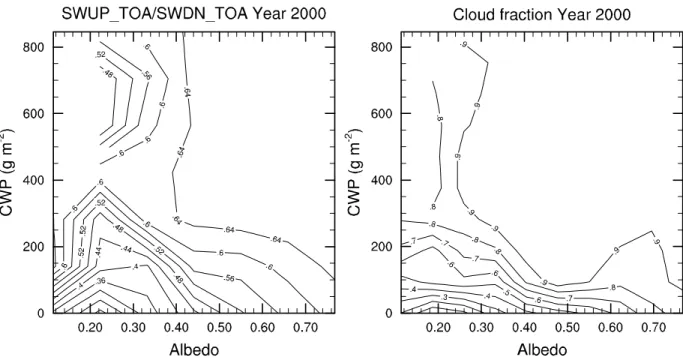
The observed radiation and cloud data are generated from the variational analysis of NWP model-produced field including ARM five sounding locations, seven NOAA wind profiler locations and RUC analysis domain over ARM SGP (Xie et al. 2004), so that cloud properties and surface albedo have same large scale temperature and moisture advective forcing, which facilitates to investigate the relationship between the surface albedo, cloud properties and radiative fluxes. Figure 11 shows normalized SWUP flux at TOA of Y1 with surface albedo and cloud water path (CWP, i.e., LWP+IWP) variations based on daily mean values for the year 2000 indicating the relationship among three variables (i.e., surface albedo, SWUP, and CWP). This figure gives a qualitative insight among the three variables. Since daily averaged quantities are used, the effect of diurnal variation by SZA change does not need to be considered. When CWP value is smaller than 400 g m-2, SWUP is slightly decreasing as surface albedo is varied up to 0.25-0.35. When the albedo is greater than 0.35, as surface albedo is increasing to larger values, SWUP tends to increase as well. There is a critical value of surface albedo for affecting SWUP flux when CWP is relatively small. On the other hand, when CWP is relatively large, it seems that SWUP increases as surface albedo does without revealing any critical value of surface
albedo. However, this is not clear in this analysis and it must be further examined whether or not the increase of SWUP at TOA is referred from the surface albedo increase when CWP is large, because optically thick cloud usually has strong reflection on its top and base. Thus, there might be critical values of surface albedo and CWP to affect SW flux, which may support the fact that more reflective surface (e.g., surface albedo is greater than around 0.35) leads to weaker SWCF at TOA with optically thin clouds, while less reflective surface (e.g., surface albedo is smaller than 0.35) does not affect cloud forcing much. Also, when the surface albedo is smaller the critical value, there is a weak decrease in SWUP at TOA with the increase of surface albedo, which suggests that a more reflective surface leads to weaker cloud forcing in thin clouds. Figure 11 also illustrates the relationship between the surface albedo, CWP and total cloud fraction. When CWP is relatively small (below 300 g m-2) and the surface albedo is large, the cloud fraction increases as the surface albedo increases, while this tendency is not clear when the surface albedo is small. It indicates that the increase of SWUP at TOA with increasing surface albedo is partly affected by the increase of cloud fraction causing stronger reflection on the cloud top when the surface albedo is large, although existing clouds are optically thin.
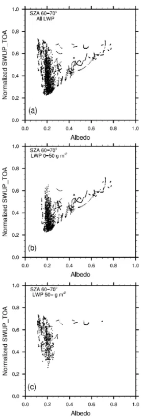
In order to specify the characteristics of surface albedo effect revealed above, it is further investigated how surface albedo is associated with SWUP at TOA considering specific ranges of LWP and SZA. Figure 12 is an example of the analysis that shows all the scattered spots on Fig. 12a can be decomposed into Fig. 12b and Fig. 12c using a critical value of LWP, i.e., 50 g m-2 in this study. SWUP at TOA is normalized by solar insolation at TOA, i.e., cloud albedo. Furthermore, Figure 12b indicates a proportional relationship between surface albedo and cloud albedo if surface albedo is larger than 0.35, otherwise less correlations between them. However, when LWP is larger than 50 g m-2 (i.e., optically thick clouds, Fig. 12c), the cloud albedo is almost constant even as surface albedo increases from 0.35 to 0.7 and has fewer correlations when surface albedo is relatively small as well. It should be noticed that surface albedo affects cloud albedo when cloud is optically thin (LWP is less than 50 g m-2) and surface albedo is larger than 0.35, otherwise if cloud is optically thick or surface albedo is small, surface albedo does not have much effect on cloud albedo. In addition, considering IWP with surface albedo and cloud albedo also shows similar characteristics. The critical values of IWP and surface albedo are 150 g m-2 and 0.35, respectively. Consequently, all the linear least-square-fit lines are calculated with all the SZA intervals considering the critical values of LWP and IWP in Fig. 13. As shown in Fig.
12, there are two regression lines for each SZA; one is for albedos from 0.1 to 0.35 and the other is from 0.35 to 0.85. There are obviously proportional relationships between surface albedo and cloud albedo when surface albedo is larger than 0.35 and LWP is smaller than 50 g m-2 (Fig. 13a). Besides as SZA increases, the slopes of regression lines decrease. However, when surface albedo is small or LWP is large, there are weak correlations between surface albedo and SWUP at TOA. IWP cases also have similar features as LWP cases do. Therefore, surface albedo strongly influences cloud albedo if cloud is optically thin (i.e., LWP and IWP is smaller than 50 g m-2 and 150 g m-2, respectively), surface albedo is greater than 0.35, and SZA is small. In other words, clouds do not affect much on the positively proportional relationship between the surface albedo and cloud albedo when the existing clouds are optically thin, surface albedo is large and SZA is small. However, if cloud is optically thick, surface albedo is small or SZA is large, the surface albedo impact on cloud albedo could be suppressed.
Furthermore at the surface, SWUP is directly proportional to surface albedo (not shown) in the all ranges of LWP and IWP, as expected, without any critical values of surface albedo, LWP and IWP. However, SWDN at the surface has similar characteristics as SWUP at TOA does (Fig. 14). SWDN at the surface is more associated with CWP rather than each LWP and IWP. This might be caused by the fact that clouds near the surface are usually constituted by both liquid and ice particles only except the summer time. Similarly as SWUP at TOA, SWDN at the surface is normalized by solar insolation at TOA. SWDN at the surface has relatively smaller correlation with surface albedo when the albedo is smaller than 0.35. Especially when CWP is greater than 180 g m-2, SWDN at the surface has little weak linear correlation with surface albedo larger than 0.35; SWDN at the surface is proportional to surface albedo as well. The correlation between them decreases as SZA increases. This result is consistent with a high-latitude case study done by Nichol et al. (2003). They explained the reason is that a great amount of surface albedo can moderate the attenuation of SW radiation by cloud through the multiple scattering between the cloud base and the surface. However, this phenomenon takes place only if optically thick cloud exists, i.e., CWP is greater than 180 g m-2, otherwise SWDN at the surface is not varied as surface albedo increases when cloud is optically thin (not shown). Thus, the reflection of cloud base could be another reason for that.
Therefore, when optically thick cloud exists, SWUP at TOA is primarily associated with the reflection of cloud top, but not much affected by the surface albedo, while the albedo influences
SWDN at the surface by the cloud base reflection and the multiple scattering between the cloud base and the surface. In other words, clouds have a negligible feedback on SWUP at TOA and slightly positive feedback on SWDN at the surface in the association with surface albedo if the cloud is optically thick. On the other hand, when optically thin cloud occurs, SWUP at TOA is mainly influenced by the surface albedo rather than cloud top reflection, while SWDN at the surface is not affected by the change as well. SWUP at the surface is generally strongly affected by surface albedo for all the cloud cases, as expected.
b. Solar zenith angle impact on surface albedo effect
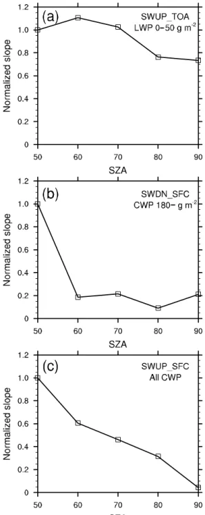
Surface albedo directly affects SW flux and SWCF, and indirectly affects cloud systems thereby influencing LW flux and LWCF also. Especially, surface albedo strongly influences SW radiative flux when SZA is small. Further analysis could be useful to quantify how those surface albedo effects depend on SZA.
As illustrated in Fig. 5, the surface albedo in Y1 simulation has clear diurnal and seasonal variation. To understand the variation quantitatively, Fig. 15 shows seasonal variation of scatter diagrams between surface albedo and cosine of SZA from Y1. Through all the seasons, surface albedo usually tends to have smaller value with small SZA than that with large SZA as similar as the illustration in Fig. 5. The numbers on each scatter diagram indicate the value of slope from linear least-square-fit calculation. The slope is relatively larger in winter revealing great dependence of surface albedo on the SZA variation mainly due to snow melting off during the daytime.
As shown in Figs. 13 and 14, the slope from linear least-square-fit regression between surface albedo and radiative fluxes could be a good parameter to quantify how the surface albedo effect on radiation depends on SZA. As revealed in the previous section, upward SW flux at TOA is significantly affected by surface albedo when optically thin clouds exist, while downward SW flux at the surface is influenced by the albedo with optically thick clouds. Also, upward SW flux at the surface is always affected by the albedo, no matter how much the existing cloud is optically thick or thin as we expected. Figure 16 illustrates normalized slopes as a function of SZA for each radiative flux. The slopes from linear least-square-fit regression between surface albedo and radiative fluxes for each SZA bin (10°) are normalized by cosine of SZA and the slope when SZA is 50°. The surface albedo effect on upward SW flux at TOA with optically thin