c
COMPILER AND RUNTIME TECHNIQUES FOR OPTIMIZING DYNAMIC SCRIPTING LANGUAGES
BY
HAICHUAN WANG
DISSERTATION
Submitted in partial fulfillment of the requirements for the degree of Doctor of Philosophy in Computer Science
in the Graduate College of the
University of Illinois at Urbana-Champaign, 2015
Urbana, Illinois
Doctoral Committee:
Professor David A. Padua, Chair, Director of Research Professor Vikram Adve
Professor Wen-Mei W. Hwu Doctor Peng Wu, Huawei
Abstract
This thesis studies the compilation and runtime techniques to improve the performance of dynamic scripting languages using R programming language as a test case.
The R programming language is a convenient system for statistical computing. In this era of big data, R is becoming increasingly popular as a powerful data analytics tool. But the performance of R limits its usage in a broader context. The thesis introduces a classification of R programming styles into Looping over data(Type I), Vector programming(Type II), and Glue codes(Type III), and identified the most serious overhead of R is mostly manifested in Type I R codes. It pro-poses techniques to improve the performance R. First, it uses interpreter level specialization to do object allocation removal and path length reduction, and evaluates its effectiveness for GNU R VM. The approach uses profiling to translate R byte-code into a specialized byte-code to improve running speed, and uses data representation specialization to reduce the memory allocation and usage. Secondly, it proposes a lightweight approach that reduces the interpretation overhead of R through vectorization of the widely usedApplyclass of operations in R. The approach combines data transformation and function vectorization to transform the looping-over-data execution into a code with mostly vector operations, which can significantly speedup the execution ofApply op-erations in R without any native code generation and still using only a single-thread of execution. Thirdly, theApplyvectorization technique is integrated into SparkR, a widely used distributed R computing system, and has successfully improved its performance. Furthermore, an R benchmark suite has been developed. It includes a collection of different types of R applications, and a flexible benchmarking environment for conducting performance research for R. All these techniques could be applied to other dynamic scripting languages.
The techniques proposed in the thesis use a pure interpretation approach (the system based on the techniques does not generate native code) to improve the performance of R. The strategy has the advantage of maintaining the portability and compatibility of the VM, simplify the implemen-tation. It is also a very interesting problem to see the potential of an interpreter.
Acknowledgments
Returning back to school to study for the Ph.D degree is a new adventure for me. This thesis dissertation marks the end of this long and eventful journey. I still clearly remember lots of sweat, pain, exciting and depressing moments in the last four years. I would like to acknowledge all the friends and family for their support along the way. This work would not have been possible without their support.
First, I would like to express my sincere gratitude to my advisor, Professor David Padua, and my co-advisor Doctor Peng Wu, for their guidance, encouragement, and immense knowledge. This thesis would certainly not have existed without their support. I also express my cordial thanks to Professor Mar´ıa Garzar´an for her help and guidance in my research. I would also like to thank my thesis committee members Professor Vikram Adve and Professor Wen-Mei Hwu, for their insightful comments and suggestions.
I am very grateful to my fellow group members and other friends in Computer Science Depart-ment. It’s my fortunate to study and research with them together.
I also thank Evelyn Duesterwald, Peter Sweeney, Olivier Tardieu, John Cohn and Professor Liming Zhang for their support in my Ph.D program. I would like to extend my thanks to Sherry Unkraut and Mary Beth Kelly for their help.
I thank my parents, who gave me the best education and built my personality.
Last but not least, special thanks to my lovely wife Bo, who inspired me and provided constant encouragement and support during the entire process.
Table of Contents
List of Tables . . . ix
List of Figures . . . x
List of Abbreviations . . . xii
Chapter 1 Introduction . . . 1
1.1 Overview . . . 1
1.1.1 Dynamic Scripting Languages . . . 1
1.1.2 R Programming Language . . . 2
1.1.3 Performance Problems of R . . . 3
1.2 Contributions . . . 5
1.3 Thesis Organization . . . 7
Chapter 2 Background . . . 9
2.1 Dynamic Scripting Language . . . 9
2.1.1 Implementation of a Dynamic Scripting Language . . . 9
2.1.2 Performance Problems of Dynamic Scripting Languages . . . 11
2.1.3 Optimization Techniques for Dynamic Scripting Languages . . . 13
2.2 R Programming Language . . . 16
2.2.1 Taxonomy of Different R Programs . . . 16
2.2.2 GNU R Implementation . . . 18
2.2.3 Performance of Type I Codes in R . . . 23
Chapter 3 Optimizing R via Interpreter-level Specialization . . . 26
3.1 Overview . . . 26
3.2 ORBIT Specialization Example . . . 28
3.3 ORBIT Components . . . 30
3.3.1 Runtime Type Profiling. . . 30
3.3.2 R Optimization Byte-code Compiler and Type Specialized Byte-code . . . 31
3.3.3 Type Inference . . . 32
3.3.4 Object Representation Specialization . . . 33
3.3.5 Operation Specialization . . . 36
3.3.6 Guard and Guard Failure Handling. . . 37
3.4 Evaluation . . . 39
3.4.1 Evaluation Environment and Methodology . . . 39
3.4.2 Micro Benchmark . . . 40
3.4.3 TheshootoutBenchmarks . . . 41
3.4.4 Other Types of Benchmarks . . . 42
3.4.5 Profiling and Compilation Overhead . . . 43
3.5 Discussions . . . 44
Chapter 4 Vectorization of Apply to Reduce Interpretation Overhead . . . 45
4.1 Overview . . . 45
4.2 Motivation. . . 48
4.2.1 RApplyClass of Operations and Its Applications . . . 48
4.2.2 Performance Issue of Apply Class of Operations . . . 49
4.2.3 Vector Programming and Apply Operation . . . 49
4.3 Algorithm . . . 50 4.3.1 Vectorization Transformation . . . 50 4.3.2 Basic Algorithm . . . 52 4.3.3 Full Algorithm . . . 54 4.4 Implementation in R . . . 61 4.4.1 Runtime Functions . . . 61
4.4.2 Caller Site Interface . . . 64
4.4.3 Optimizations. . . 64
4.5 Evaluation . . . 67
4.5.1 Benchmarks. . . 67
4.5.2 Evaluation Environment and Methodology . . . 68
4.5.3 Vectorization Speedup . . . 68
4.5.4 Overhead of Data Transformation . . . 69
4.5.5 Vectorization of Nested Apply Functions . . . 71
4.5.6 Vector Programming in the Applications. . . 72
4.5.7 Tiling in Vectorization . . . 72
4.5.8 Built-in Vector Function’s Support . . . 74
4.6 Discussions . . . 75
4.6.1 Pure R Based Implementation . . . 75
4.6.2 Combine Vectorization with Parallelization . . . 75
4.6.3 Different to Conventional Automatic Vectorization . . . 76
4.6.4 Limitations . . . 76
4.6.5 Extended to Other Dynamic Scripting Languages . . . 77
Chapter 5 R Vectorization in Distributed R Computing Framework . . . 79
5.1 Introduction . . . 79
5.2 SparkR Background . . . 81
5.2.1 Basic Structure . . . 82
5.2.2 SparkR APIs . . . 83
5.3 Integration R Vectorization to SparkR . . . 85
5.3.1 Function Vectorization . . . 86
5.3.2 Data Transformation . . . 86
5.3.3 Caller Site Rewriting . . . 87
5.3.4 Other Transformations . . . 87
5.3.5 Optimizations. . . 88
5.3.6 Code Transformation Example - Linear Regression . . . 89
5.4 Evaluation . . . 89
5.4.1 Benchmarks. . . 89
5.4.2 Evaluation Environment . . . 91
5.4.3 Evaluation Methodology . . . 91
5.4.4 Vectorization Speedup . . . 92
5.4.5 Comparing with Manually Transformed Vector Code . . . 94
5.4.6 Comparing with Single Node Standalone R . . . 95
5.5 Discussion. . . 97
Chapter 6 R Benchmark Suite . . . 102
6.1 Introduction . . . 102 6.2 Benchmark Collections . . . 103 6.3 Benchmarking Environment . . . 105 6.3.1 Application Interface . . . 106 6.3.2 Benchmark Driver . . . 106 6.3.3 Benchmark Harness . . . 107 6.4 Discussion. . . 108
Chapter 7 Related Work . . . 109
7.1 Optimizing R Language . . . 109
7.1.1 The Landscape of Existing R Projects . . . 109
7.1.2 Building new R Virtual Machines . . . 109
7.1.3 Extensions/Variations to the GNU R . . . 111
7.2 Optimization in Dynamic Languages . . . 112
7.2.1 Interpreter. . . 112
7.2.2 Runtime Optimization . . . 113
7.2.3 JIT Native Code Generation . . . 113
7.2.4 Ahead-of-time (AOT) Compilation . . . 113
7.3 Performance Improvement through Vectorization . . . 114
7.3.1 Function Vectorization . . . 114
7.3.2 Vectorization in Scripting Language . . . 114
7.4 Parallel and Distributed R Processing System . . . 115
7.4.1 Parallel R System . . . 115
7.4.2 Distributed R System . . . 115
Chapter 8 Conclusions. . . 117
8.1 Summary . . . 117
List of Tables
2.1 Number of machine instructions executed and object allocated for the example in
Figure 2.4. . . 25
3.1 Instrumented R Byte-code instructions in ORBIT . . . 31
3.2 Percentage of memory allocation reduced forscalar. . . 41
3.3 Metrics of Optimized For-loop Accumulation . . . 41
3.4 Percentage of memory allocation reduced forshootout. . . 42
3.5 Runtime measurements offannkuch-redux . . . 43
4.1 Apply Family Operations in R . . . 48
4.2 Data Representation of Different Types . . . 55
4.3 R Functions Supporting Direct Replacement . . . 63
4.4 Benchmarks and configurations. . . 67
4.5 Data transformation overhead (Iterative benchmarks) . . . 70
4.6 Data transformation overhead (Direct benchmarks, Base Input) . . . 70
5.1 Benchmarks and Configurations . . . 91
5.2 Software configuration in SparkR evaluation . . . 91
List of Figures
1.1 Software used in data analysis competitions in 2011[45] . . . 3
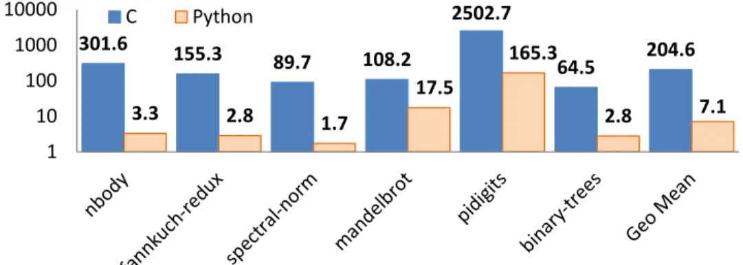
1.2 Slowdown of R on theshootoutbenchmarks relative to C and CPython.. . . 4
2.1 Three different R programming styles. . . 17
2.2 The GNU R VM. . . 18
2.3 Slowdown of R AST Interpreter of theshootout benchmarks relative to C and CPython. . . 19
2.4 R byte-code and symbol table representation. . . 20
2.5 Internal representation of R objects. . . 20
2.6 Local Frame Structure . . . 21
2.7 Matrix Structure . . . 22
2.8 R Copy-on-Write Mechanism. . . 23
3.1 Specialization in ORBIT VM . . . 28
3.2 An example of ORBIT specialization. . . 28
3.3 The ORBIT VM. . . 30
3.4 The type system of ORBIT. . . 33
3.5 The VM stack and type stack in ORBIT. . . 34
3.6 States of Unboxed Valued Cache . . . 35
3.7 Speedups on thescalarbenchmarks. . . 40
3.8 Speedups on theshootoutbenchmarks. . . 42
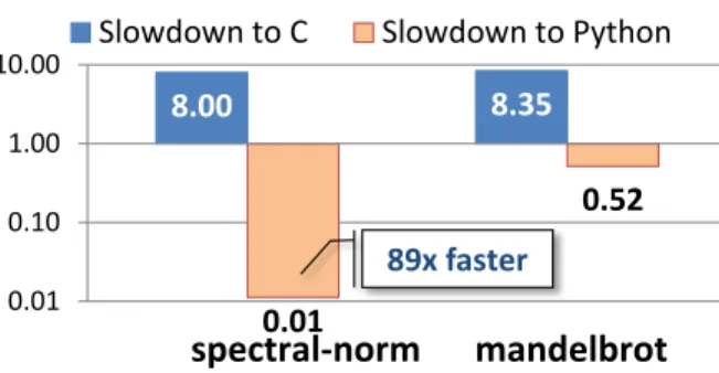
4.1 Slowdown of R on twoshootoutbenchmarks relative to C and CPython. . . 46
4.2 Function Vectorization Transformation . . . 51
4.3 Loop Distribution in Vectorization Transformation . . . 54
4.4 Three Tasks in the Full Vectorization Algorithm . . . 55
4.5 Data Access afterPERM DOWNTransformation . . . 56
4.6 Function Vectorization Transformation Example. . . 60
4.7 Speedup ofApplyoperation vectorization (Iterative benchmarks) . . . 69
4.8 Speedup ofApplyoperation vectorization (Direct benchmarks) . . . 69
4.9 Speedup of different levels’ Apply vectorization . . . 71
4.10 Speedup of different vector lengths (Base Input) . . . 73
4.11 Speedup of Different Tiling Sizes (Base Input). . . 73
5.2 Parallel Computing of R based on Distributed Runtime System . . . 80
5.3 SparkR Architecture and Object Storage . . . 82
5.4 RDD Data Vectorization . . . 86
5.5 Speedup of vectorization in SparkR . . . 93
5.6 Speedup of the vectorized LogitReg to the manually written vector LogitReg . . . 95
5.7 Speedup of SparkR to standalone R . . . 99
5.8 Speedup of vectorized SparkR to vectorized standalone R . . . 100
5.9 Absolute running time(second) of standalone R and SparkR. . . 101
6.1 Benchmarking Environment . . . 105
6.2 The Delta Approach in the Benchmarking . . . 107
List of Abbreviations
AOT Ahead of Time Compilation. AST Abstract Syntax Tree.
CFG Control Flow Graph.
CRAN the Comprehensive R Archive Network DSL Dynamic Scripting Language.
GPU Graphics Processing Unit. IR Intermediate Representation. JIT Just-In-Time Compilation.
SIMD Single Instruction, Multiple Data.
Chapter 1
Introduction
1.1
Overview
1.1.1
Dynamic Scripting Languages
Dynamic Scripting Languages are generally used to refer programming languages with features like dynamic evaluation (without Ahead-Of-Time compilation), high level abstraction and con-cepts, dynamic typing, and managed runtime. Examples of popular dynamic scripting languages include JavaScript, Python, PHP, Ruby, Matlab, R, etc.. These languages are becoming more important in the programming language spectrum recently years. About half of the top 10 most popular programming languages in both the TIOBE programming community index[30] and the IEEE Spectrum list[74] are dynamic scripting languages. Many dynamic scripting languages have been widely adopted including JavaScript for web client interface, PHP and Ruby for web front-end applications, Matlab for technical computing, R for statistic computing, and Python for a wide range of applications.
However, there is still one major problem that inhibits the pervasive usage of dynamic script-ing languages, the relatively low performance compared with their static language counterpart. The shootout benchmark[4] report shows that an implementation of some common algorithms in dynamic scripting languages is typically over 10x slower than the implementation in static lan-guages. There are mainly two reasons for the low performance. First, theinterpretation overhead
since most of the scripting languages are interpreted in a managed environment. Secondly, the
Many approaches have been proposed to reduce the two kinds of overheads in the past decades, such as Just in Time Compilation (JIT) and Specialization. These techniques greatly improved the performance of dynamic scripting languages although there are still many unsolved problems.
1.1.2
R Programming Language
Thanks to the advent of the age of big data, R[14] has become a rising star among the popular dynamic scripting languages. R is a tremendously important language today. According to the NY times [81]:
R is used by a growing number of data analysts inside corporations and academia. It is becoming their lingua franca partly because data mining has entered a golden age, whether being used to set ad prices, find new drugs more quickly or fine-tune financial models. Companies as diverse as Google, Pfizer, Merck, Bank of America, the InterContinental Hotels Group and Shell use it.
In other words, the reason for the growing importance of R is the emergence of big data. In the case of business, this emergence is leading to a revolution that shifts the focus of information pro-cessing from the back-office, where work was carried out by traditional data propro-cessing systems, to the front-office where marketing, analytics, and business intelligence [59] are having a growing impact on everyday operations.
One illustration of R’s popularity is that most of the competitors on Kaggle.com, the No.1 online website in solving business challenges through predictive analytics, use R as their tools to solve the contest problems[7]. In fact, the number of R users in Kaggle.com is significantly higher than the number of users of other languages, such as Matlab, SAS, SPSS or Stata, (see Figure1.1). R can be considered as the lingua franca for data analysis today, and is therefore of great interest. Today, there are more than two million users of R, mainly from the field of data analysis, a scientific discipline and industry that is rapidly expanding. According to [73]:
Figure 1.1: Software used in data analysis competitions in 2011[45]
Long gone are the days when R was regarded as a niche statistical computing tool mainly used for research and teaching. Today, R is viewed as a critical component of any data scientist’s toolbox, and has been adopted as a layer of the analytics infras-tructure at many organizations
The popularity of R is mainly due to the productivity benefits it brings to data analysis. R contributes to programmer productivity in several ways, including the following two: the avail-ability of extensive data analysis packages that can be easily incorporated into an R script and the interpreted environment that allows for interactive programming and easy debugging.
1.1.3
Performance Problems of R
The downside, and the justification for this thesis, is that R shares the limitations of many other interactive and dynamically typed languages: it has a slow implementation1. Unfortunately the
performance of R is not properly understood. Some reported orders of magnitude slowdowns of R compared to other languages. Figure 1.2 compares the performance of a set of common 1R language has only one official implementation GNU R. The performance of R in this thesis refers the perfor-mance of GNU R
algorithms [4] implemented in different languages. It shows that for the implementations of those algorithms, R is more than two orders of magnitude slower than C and twenty times slower than Python (also an interpreted scripting language). Not only is R slow, it also consumes a significant amount of memory. All user data in R and most internal data structures used by the R runtime are heap allocated and garbage collected. As reported in [61], R allocates several orders of magnitude more data than C. Memory consumption is both a performance problem (as memory management and data copying contribute to the runtime overhead) and a functional problem (as it limits the amount of data that can be processed in memory by R codes). To cope with the performance and memory issues of R, it is a common practice in the industry for data scientists to develop initial data models in R then have software developers convert R codes into Java or C++ for production runs. 301.6 155.3 89.7 108.2 2502.7 64.5 204.6 3.3 2.8 1.7 17.5 165.3 2.8 7.1 1 10 100 1000 10000 C Python
Figure 1.2: Slowdown of R on theshootoutbenchmarks relative to C and CPython.
In contrast, some users claimed that their R codes run as fast as any native code and are indeed used in production. Both claims are partially true since the performance or R codes depends on how the R codes are written.
R programs can be classified into three categories[84], Type I (looping over data), Type II (vector programming), and Type III (glue codes). The evaluation shows that the significant perfor-mance problems only appear in Type I R codes. The perforperfor-mance gap between R and C/Python showed in Figure1.2 are the result of the Type I programming. Type II codes are much more ef-ficient compared with Type I. These codes mainly suffer the performance problems of losing data
locality due to long vector computation. Finally, Type III codes’ performance is purely dependent on the back-end implementation (in C and FORTRAN) of the R library, and it belongs to the static language domain.
While many R users are forced to use the Type III style in production codes due to the heavy overhead of Type I and II codes, according to [61], a significant portion of R codes still spend most of the execution time in Type I and II codes. And it is a common practice that Type I and Type II R codes are rewritten using other languages for production environment due to the slowness and memory consumption of R codes. Clearly, there are great benefits in having a highly efficient implementation of R for Type I and II codes so that R can be a productive programming environment where glue codes and main computation can be implemented in a uniform fashion.
1.2
Contributions
This thesis studies the compilation and runtime techniques to improve the performance of dynamic scripting languages. It makes the following contributions to tackle the poor performance problems of R:
• Allocation removal and path length reduction via interpreter-level specialization
This thesis describes an optimized R byte-code interpreter, named ORBIT (Optimized R Byte-codeInterpreTer). ORBIT is an extension to the GNU R VM. It performs aggressive removal of object and reduction of instruction path lengths in the GNU R VM via profile-driven specialization techniques. The ORBIT VM is fully compatible with the R language and is purely based on interpreted execution. It uses a specialization JIT and runtime that focus on data representation specialization and operation specialization. For the benchmarks of Type I R codes, the current ORBIT is able to achieve an average of 3.5X speedups over the GNU R VM and outperforms on the average most other R optimization projects that are currently available.
• Vectorization of R Apply operations to reduce interpretation overhead
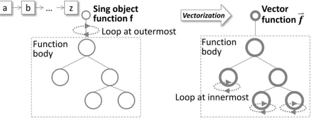
This thesis presents a lightweight approach that reduces the interpretation overhead of R through the vectorization of the widely usedApply class of operations in R. The normal implementation of Apply incurs in a large interpretation overhead resulting from itera-tively applying the input function to each element of the input data. The proposed approach combines data transformation and function vectorization to transform the looping-over-data execution into a code with mostly vector operations, which can significantly speedup the execution ofApplyoperations in R.
The vectorization transformation has been implemented as an R package that can be invoked by the standard GNU R interpreter. As such, the vectorization transformation does not re-quire any modification to the R interpreter itself. The package automatically vectorizes the
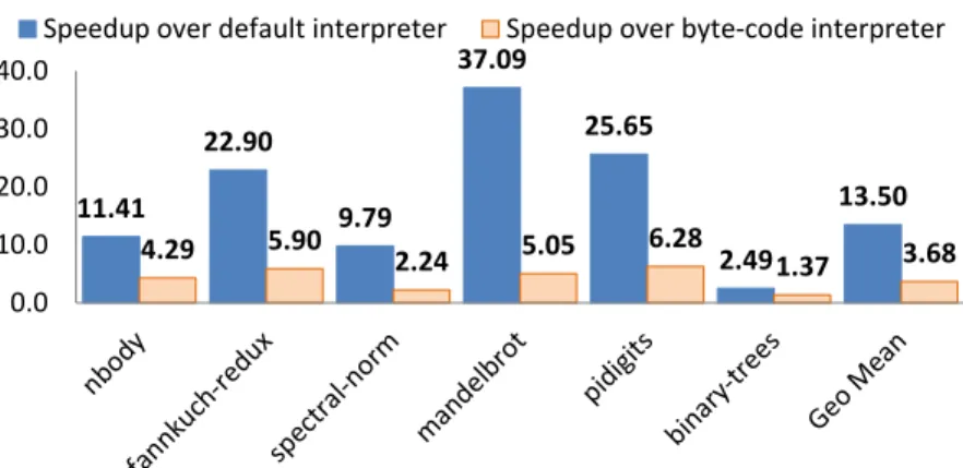
Applyclass of operations. The evaluation shows that the transformed code can achieve up to 22x speedup (and 7x on average) for a suite of data analytics benchmarks without any native code generation and still using only a single-thread of execution.
• Improving distributed R computing systems with operation vectorization
New compiler transformations are presented that improves the performance of SparkR[82], by extending the Apply vectorization technique just discussed into a two-level compiler transformation. The outer level is used to distribute data and computation while the inner level to reduce interpreter overhead. This transformation integrated with the SparkR inter-faces. A two-levelReduceschema is also used to get the correct result. With these trans-formations, the SparkR’s performance is doubled in the benchmark composed by a bunch of distributed algorithms.
• Portable R benchmark suite and benchmarking environment
A suite of micro-benchmarks was developed as well as an R benchmarking environment. One challenge we face in the study of strategies for improving R performance is the lack
of a proper performance benchmarks for R. Another problem is that different R language implementations have different interfaces which causes the comparison of different R opti-mization techniques hard to conduct. Based on the classification R programs into Type I, II, and III styles, a collection of different types of R applications was developed and standard-ized. This collection is expected to facilitate researchers in this domain to locate the proper optimization targets. Furthermore, a flexible R benchmarking environment is provided to enable different R implementations to be measured with the benchmarks in the same man-ner. The benchmarking environment can be extended by plugging in additional meters to measure performance metrics such as Operation System data and hardware performance counters. The benchmark suite and benchmarking environment can help researchers in this domain easily get deep understanding of R’s behaviors.
1.3
Thesis Organization
The remainder of the thesis is structured into chapters as follows:
• Chapter2: Discusses the high-level background of the implementation and common opti-mizations for dynamic scripting languages. Then it describes the GNU R Virtual Machine (VM) structure, analyzes the performance issues for better understanding the approaches proposed in this thesis.
• Chapter 3: Describes the new interpreter level specialization techniques, including byte-code specialization and object representation specialization, and the implementation of these techniques in ORBIT VM.
• Chapter4: Introduces the vectorization transformation ofApplyoperations in R, includ-ing the transformation framework, operation and data transformation algorithms, and the realization of the transformation in an R library.
• Chapter5: Describes the compiler transformations and runtime optimizations used in ap-plying vectorization into the SparkR distributed computing system.
• Chapter6: Introduces the R benchmark suites as well as the R benchmarking environment. • Chapter7: Discusses the related work in dynamic scripting language domain and
optimiza-tion work in R language area.
Chapter 2
Background
This chapter discusses the topics that help understand the remainder of the thesis. First, it describes the high level components that are required in implementing a dynamic scripting language. The typical performance problems and the common optimization techniques are introduced then. Sec-ondly it gives a brief introduction of the R language, and explains the the GNU R Virtual Machine (VM) structure, analyzes the performance issues, and the optimizations used in GNU R VM.
2.1
Dynamic Scripting Language
2.1.1
Implementation of a Dynamic Scripting Language
Like static languages such as C and Java, the basic structure of implementation a dynamic scripting language (DSL) is similar. The source code is translated into the executable control sequences that the underlying hardware can understand and execute. This requires the compiler path (lexer, parser, optimizer, etc.). A dynamic language also requires object descriptors to enable the identification of different types of objects. Furthermore, the language implementation needs other components to handle tasks such as code loading, interface with other languages, etc..
Furthermore, DSLs have many unique language features, which require special implementa-tions. The following section describes a few common components used in realizing a DSL.
Interpreter In many usage scenarios, the source code of a DSL program is input dynamically, which means an Ahead-Of-Time (AOT) compilation cannot be conducted. An interpreter is com-monly used to handle this situation. The interpreter accepts the source code’s representation in the
form of an Abstract Syntax Tree (AST) or byte-code program, and evaluates it.
There are two types of interpreters, AST interpreters and byte-code interpreters. An AST interpreter will traverse the AST top-down to trigger the evaluation of the current node’s child nodes, and merge the result bottom-up to get the final result. Like static languages, the AST of a DSL can also be translated into a sequence of instructions, called code. However, these byte-code program will not be executed by the bare hardware processor, but by a software implemented virtual machine(VM). The VM has implements the logic of each byte-code instruction, and it interprets the byte-code one instruction at a time, modifies the VM runtime environment, and finally gets the result in the memory or the VM stack.
Generic Object Representation Similar to static languages, dynamic scripting languages typ-ically have many different types, such as boolean, integer, string, etc. However, many of these languages have the feature that only values carrie the type, not the variable, which means a vari-able can be bound to different values with different types at different time. Because the type of a variable cannot be decided statically, a common implementation in dynamic scripting languages is to use generic representation to describe a value object (typically a class with one field to describe the type, and one field to store the real raw data). Because the size of the generic representation cannot be decided statically either, objects are dynamically allocated in the heap by most imple-mentations.
Furthermore, many dynamic languages contain extensible data types, for example a value in JavaScript can contain arbitrary numbers of fields, and a value in R can be set with arbitrary numbers of attributes. In order to represent these types, a map or a linked list structure is commonly used to implement these types.
Dynamic Dispatch Because the variable in dynamic languages does not carry type, the opera-tions on the variable cannot be decided statically. For example consider anadd operation in the JavaScript expression a+b. Ifa and bare both numbers, the addition will do number addition
(64bit floating point addition). But ifaandbare all strings, the addition will do string concatena-tion. And ifais a string whilebis a number, the addition operation will first promote the number into a string, then do string concatenation. The operation of the addition is dynamically decided according to the types of the input operands. The mechanism is similar to the implementation of polymorphic operation in object-oriented programming, and is also called dynamic dispatch here.
Dynamic Variable Lookup A variable in a DSL may be or not be defined at a specific point in the source code. So a common practice in the implementation is not to have static binding for a variable. As a result, unlike static languages, where a variable can be located through a fixed index offset, there is no fixed index to locate a variable in the corresponding context frame (a method’s local frame or the global frame). The common implementation is using the variable’s name to do a runtime lookup, and find the current bound location to get the value.
Dynamic Memory Management and Garbage Collection Because most of the objects and resources are allocated dynamically, there are far fewer memory regions allocated statically in a DSL. Most of the memory allocation requests are resolved as a heap allocation, and require the language’s runtime to handle the allocation and de-allocation. In order to reduce the burden of the programmer, Garbage Collection(GC) is typically used by a DSL, although this is not unique to DSLs. Many static languages also have Garbage Collection, such as Java.
2.1.2
Performance Problems of Dynamic Scripting Languages
As described in Chapter1, dynamic scripting languages have the benefit of providing interactive programming environment, high level abstraction and high productivity. The major limitation for pervasive of these languages is the low performance. According the data reported in the shootout benchmark website[4], the speed performance gap between dynamic scripting languages and static languages is typically 10x or higher. This is mainly due to their implementation as described in Section2.1.1.
Interpretation Overhead The interpreter is indeed a software simulated processor to execute the language’s instruction sequence. The byte-code interpreter is very similar to the hardware proces-sor, which performs the tasks of fetching a byte-code, decoding the byte-code, loading operands, performing the computation and storing the result back. Each step requires the execution of many real native instructions, which are all overhead compared with a pre-compiled native binary from a static language. The AST interpreter has even higher overhead since it has to traverse the AST through all kinds of pointers. This kind of traversing is tedious and lack of locality.
Memory Management Overhead Because of the generic object representation, most of the ob-ject types are expressed as a Boxed obob-ject. For example, a primitive integer is not just a 32bit memory cell in the stack or heap, but a class object that contains the header (type and size at-tributes) and the raw data. An additional pointer is required to refer the class object, and the object is commonly allocated in the heap. All of these incur memory usage overhead as well as the need to execute additional instructions to traverse the pointers and get the real type and value.
Dynamic Dispatch Overhead Due to the dynamic dispatch attribute, the logic to implement the dynamic dispatch either contains a large control flow to check the types and invoke the cor-responding routines, or a dispatch table lookup that still requires a table lookup and execution of comparison operations. This not only increase the native instruction path length but also slow down the hardware processor’s pipeline due to the complex control flows.
Variable Lookup Overhead Because there is no fixed index for a variable in a frame, a variable lookup requires a dynamic search in the runtime environment. The lookup operation is imple-mented either a hashmap search or a linear search. In either way, a string comparison is required, which has to use many native instructions to get the result. Considering variable read and write are the most frequent operations in the program, the overhead is very large.
Memory Management Overhead This overhead comes from the heap allocation of nearly all the dynamic resources as well as the garbage collection time for them.
2.1.3
Optimization Techniques for Dynamic Scripting Languages
There are many optimization techniques for dynamic scripting languages, starting from the early research on Smalltalk[40] and SELF [33][32]. The most common used approaches in the modern dynamic scripting languages are briefly described here.
Byte-Code Interpreter The easiest to build are the AST interpreters. However, due to the rea-sons explained in the previous section, AST interpreters have very poor performance. One com-mon optimization is to translate the program AST into a byte-code sequence, and let it be executed in a byte-code interpreter. The interpretation logic of each byte-code instruction is relatively simple and can be implemented efficiently. Furthermore the linear execution of the byte-code sequence has better locality compared with the tree traversal in the AST interpreter. As a result, a byte-code interpreter is typically much faster than an AST interpreter.
Threaded Code A simple byte-code interpreter uses a switchstatement to do the byte-code dispatch. This approach requires a large dispatch table and numerous comparisons, which cause poor hardware processor pipeline performance. Threaded code[26] is used to optimize the dis-patch. The basic idea is that each byte-code instruction has a field to store the interpretation code’s address for the next byte-code instruction. After interpreting the current instruction, there is no need to jump back to the big switch to do the dispatch, but directly jump to the next byte-code instruction’s interpretation logic. Depends on where the next byte-byte-code’s address is stored, where the operands of an instruction are stored, and how the byte-code execution logic is invoked, threaded code can be implemented as direct threading, in-direct threading, subroutine threading, token threading, etc..
Specialization Because of the dynamic type feature, the execution logic of one operation in a dynamic scripting language typically consists all the combinations of routines to process different types. The implementation has many type checks, branches, and unbox routines (to handle boxed object representations). Specializationis a general term to describe the approach that capture the behaviors of the real execution for a particular operand type combination with a special routine for each combination. The special routine have much simpler logic, less checks. On the negative side, they require a predicate to guard that the operands have the expected type. For example, if both
aandbin thea+b expression of Section2.1.1are integers, a special routine to do integer addi-tion is provided for better performance. Specializaaddi-tion is commonly based ontypesand contexts, where the types could be variable types or function types. As a result, specialization typically requires type analysis or type inference. The implementation of specialization may contain oper-ation side specializoper-ation (generating different instruction sequences), memory side specializoper-ation (define special object representations).
Inline Cache Inline Cache was introduced to optimize the polymorphic procedures invocations in Smalltalk[37]. It is also used to handle the dynamic dispatch in dynamic languages in a similar fashion[48]. It is based on the observation that the object type for a dynamic dispatch is relatively stable at a specific instruction location. So a cache could be allocated there to store last time’s invocation target. In the next execution at the same location, if the check proves the type is not changed, the execution can directly invoke last time’s target without the expensive dynamic lookup. Besides the dynamic dispatch, inline cache can also be used to accelerate the access of a object field in a dynamic shaped object. For example, accessing the fieldaof the variablevar1through
var1.b. The simple implementation of object var1 is a table or a map. Every field access requires a heavy name based lookup, comparing each entry in the table or map. If it finds one entry’s name isb, the value of that entry is returned. With the hidden class optimization support, the field access can be transformed as a integer offset based lookup, and use inline cache to cache last time’s offset.
Hidden Class Hidden Class was firstly used in SELF implementation[33] to accelerate the dy-namic object’s field access. If the language has the feature that one object can contain an arbitrary number of fields, the simple implementation is to use a table or a map to represent the object. Then the accessing a field would be is slow due to the need of table/map entry lookup. The fact that a piece of code has a relatively stable field access that enable the optimization described next. Consider a function with input argument arg, in which arg.a field is accessed first, and then thearg.b. If there is a class (like a class in a static language) to define the type of the variable
arg, the field access can be changed to a fixed index lookup in the class instance. Hidden class approach tries to abstract the class structure from the execution sequences. During the execution, a tree of classes are generated. The parent to children linkage is typically based on the field access sequence. Then the most precise class to describe a object is found, and the field access can be ac-cessed using a fixed offset in the class structure, and can be further optimized with the combination of Inline Cache.
JIT Just-In-Time compilation is commonly used in the optimization of dynamic scripting lan-guages. Based on the feedback from the interpreter, for example the code execution frequency, the type information traced or profiled, the code is then passed into a runtime compiler. The compiler applies code optimizations and generates more efficient code sequences for the next time’s execu-tion. The more efficient code sequence could be but not limited to native instructions. Other kinds of representation is possible, for example, JIT AST code into byte-code. Depends on the scope of the compiler transformation, JIT can be implemented as trace JIT (linear sequence of instructions, across method boundary), method level JIT, code block JIT (for example, only a loop region).
Native Code Generation Native code generation is also called machine code generation. It translates the code executed in the interpreter to native code sequence and runs it directly on the bare processor. It removes the interpretation overhead. However, if other optimizations are not applied during the native code generation, the runtime overhead is still there. Typically, native
code generation is the last step of dynamic scripting language optimization. It has the advantage of removing the interpretation overhead, but also has the limitation of architecture dependent.
2.2
R Programming Language
R language belongs to the dynamic scripting language domain. It is based on the S language [34] from Bell Labs, and originally developed by Ross Ihaka and Robert Gentleman, where the nameR
comes from. It is now developed and maintained by a small group of about twenty people around the world, which is called R core team. It is traditionally used in statistics domain, and has been becoming very popular recently years in data science and other domains.
[13] has describes the language in detail, and [61] gave a detail evaluation of the language from a programming language design perspective. This section only describes some important features and implementations of R regarding the thesis work.
2.2.1
Taxonomy of Different R Programs
R is not only a dynamic scripting language, but also a vector language. It has built-in vector, matrix and high-dimension array support. It also has many native languages (C and FORTRAN) implemented libraries wrapped as packages. Based on how programmer write R programs, there are three distinct R programming styles. Figure2.1shows the examples. Each exhibits a different performance trait and requires drastically different approaches to performance optimization:
• Type I: Looping over data. This programming style, as shown in Listing2.1, is the most natural programming style to most users but is also the worst performing among the three programming styles. This comes mainly from the overhead of operating on individual vector elements in R. The several orders of magnitude of performance gap shown in Figure 1.2 ensues from the fact that the codes in that figure are all of Type I.
1 # ATT bench: creation of Toeplitz matrix 2 for (j in 1:500) { 3 for (k in 1:500) { 4 jk<-j - k; 5 b[k,j] <- abs(jk) + 1 6 } 7 }
Listing 2.1: Type I: Looping Over Data
1 # Riposte bench: age and gender are long vectors
2 males_over_40 <- function(age, gender) {
3 age >= 40 & gender == 1
4 }
Listing 2.2: Type II: Vector programming
1 # ATT bench: FFT over 2 Million random values
2 a <- rnorm(2000000);
3 b <- fft(a)
Listing 2.3: Type III: Glue codes
Figure 2.1: Three different R programming styles.
• Type II: Vector programming.In this programming style one writes R codes using vector operations as shown in Listing2.2. When operating mainly on short vectors, Type II codes suffer similar performance problems as Type I codes (henceforce, Type I also refers short vector Type II). When applied to long vectors, Type II codes are much better performing, but may suffer from poor memory subsystem performance due to loss of temporal locality in a long vector programming style.
• Type III: Glue codes. In this case R is used as a glue to call different native implemented libraries. List 2.3shows such an example, wherernorm() andfft()are native library routines. The performance of Type III codes depends largely on the quality of native library implementations.
2.2.2
GNU R Implementation
There is only one official implementation of R language, the CRAN R project [14], and the R language itself is defined by this implementation. A brief introduction of GNU R virtual machine with its object representation is described below.
R Source Code Parser R AST Byte-code
Compiler R Byte-code
Pre-compiled packages
AST Interpreter Byte-code Interpreter
R Runtime Environment
(Local frames, global frames, built-in function objects)
Figure 2.2: The GNU R VM.
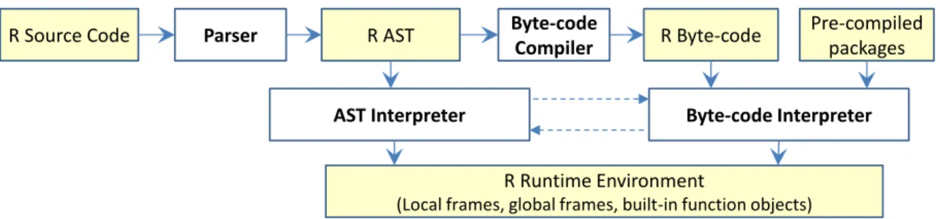
Figure 2.2 depicts the structure of the GNU R VM since version R-2.14.0 that includes a parser, two interpreters, and a runtime system that implements the object model, basic operations, and memory management of R.
AST Interpreter and Byte-code Interpreter
TheR AST interpreteris the default interpreter used by the GNU R VM. This interpreter operates on the Abstract Syntax Tree (AST) form of the input R program and is very slow. Figure2.3shows the R AST interpreter’s performance comparing to C and CPython. The slowdown is even larger than the number shown in Figure1.2, where the R byte-code interpreter is used. Since R version 2.14.0, a stack-basedR byte-code interpreter[77] was introduced as a better performing alternative to the AST interpreter. To enable the byte-code interpreter, the user has to explicitly invoke an interface to compile a region of R code into byte-codes for execution or set an environment variable to achieve the same goal. Since the two interpreters use the same object model and share most of the R runtime, it is possible to switch between the two interpreters at well-defined boundaries such as function calls.
801.3 603.5 392.4 794.2 10212.4 117.5 752.0 8.8 11.1 7.6 128.2 674.5 5.1 26.2 1 10 100 1000 10000
100000 Slowdown to C Slowdown to Python
Figure 2.3: Slowdown of R AST Interpreter of the shootout benchmarks relative to C and CPython.
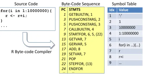
The byte-code interpreter has a simple ahead-of-time (AOT) compiler that translates ASTs generated by the parser to byte-codes. For each function, the R byte-code compiler produces two components, the symbol table and the byte-code. The symbol table records all the variable names, constant values and expressions in the source code. The byte-code instruction uses the symbol table to look for a value. Figure2.4shows an example byte-code sequence and the corresponding symbol table. The detail R byte-code compiler and byte-code format can be found at [78]. The AOT compiler also performs: simple peephole optimizations, inlining of internal functions, faster local variable lookup based on predetermined integer offset, and specialization of scalar math expressions. For Type I codes, the byte-code interpreter is several times faster than the AST interpreter. Starting from R-2.14.0, many basic R packages are compiled into byte-codes during installation and executed in the byte-code interpreter.
However, the compilation into byte-code is purely ahead of time, all the byte-codes are type generic, which still requires dynamic type checking and dispatching. Furthermore, the byte-code interpreter does not change the GNU R runtime implementation, and it still suffers the same issues from the runtime as the AST interpreter.
Idx Value 1 ‘:’ 2 1 3 10000000 4 1:10000000 5 i 6 for(i in …){…} 7 r 8 r+i 9 … STMTS GETBUILTIN, 1 PUSHCONSTARG, 2 PUSHCONSTARG, 3 CALLBUILTIN, 4 STARTFOR, 6, 5, (22) GETVAR, 7 GERVAR, 5 ADD, 8 SETVAR, 7 POP STEPFOR, (13) ENDFOR Byte-Code Sequence PC 1 3 5 7 9 13 15 17 19 21 22 24 ... ... Symbol Table Source Code for(i in 1:10000000){ r <- r+i; } ... R Byte-code Compiler
Figure 2.4: R byte-code and symbol table representation.
SEXPREC VECTOR_SEXPREC sxpinfo_struct sxpinfo SEXPREC* CAR SEXPREC* CDR SEXPREC* TAG SEXPREC* attrib SEXPREC* pre_node SEXPREC* next_node sxpinfo_struct sxpinfo SEXPREC* attrib SEXPREC* pre_node SEXPREC* next_node R_len_t length R_len_t truelength
Vector raw data
SE X PRE C_ H EA D ER
Figure 2.5: Internal representation of R objects.
R Object Model
The GNU R VM defines two basic meta object representations:SEXPREC(henceforth referred to asNodeobject for short) and VECTOR SEXPREC(henceforth referred to as VECTOR orVector
object for short). As shown in Figure 2.5, an object has an object header (SEXPREC HEADER) and a body. The object header is same for both SEXPREC and VECTOR. The header contains three pieces of information:
• sxpinfothat encodes the meta data of an object such as data type and object reference count • attribthat records object attributes as a linked list
• prev nodeandnext nodethat link all R objects for the garbage collector
The VECTORdata structure is used to represent vector and matrix objects in R. The body of theVECTORrecords vector length information and the data stored in the vector. Scalar values are represented as vectors of length one.
TheSEXPRECdata structure is used to represent all R data types not represented by VECTOR such as linked-list and internal R VM data structures such as the local frame. The body of SEX-PRECcontains three pointers toSEXPRECorVECTORobjects:CAR, CDR, and TAG. Using the three pointers, a linked-list can be easily implemented bySEXPRECin a LISP style.
Figure2.6shows a local frame represented as a linked list of entries where each entry contains pointers to a local variable name, the object assigned to the local variable, and the next entry in the the linked list. And an environment is composed by several local frames, where in each frame’s head node, one pointer points to the local frame linked list, one points to its parent frame, and the last one points to a hash table for fast object lookup.
Node
Node Node Node
Vector (string) Vector (double) Hashmap cache ‘r’ 1000 … … … Parent frame Current frame r <- 1000
Figure 2.6: Local Frame Structure
Figure2.7presents the structure a matrix is expressed with theNodeobject andVectorobject. A matrix uses a VECTOR object as the base, and the attrib field in the base object’s header points to a linked list, where a dim attribute binding is defined. The name of the binding is a length-three string vector (“dim”), and the value of the binding is a length-two integer vector ([3,4]), which is used to define the first dimension and the second dimension sizes of the matrix.
Although the LISP like data structure is flexible and can represent arbitrary R objects, it also causes serious performance issues. Thus, traversing the linked structure requires the execution of numerous instructions. And the big header consumes much space even for simple type objects,
Vector (double) Node Vector (string) Vector (integer) 1:12 … attrib ‘dim’ 3,4 matrix(1:12, 3, 4)
Figure 2.7: Matrix Structure
such as simple scalars and vectors. Furthermore, the SEXPREC node object are heavily used everywhere as the construction units for all other data type objects. As a result, the whole heap of R runtime is composed by huge amount of smallSEXPRECandVECTORobjects.
Memory Management
Memory Allocator The memory allocator of R VM pre-allocates pages ofSEXPREC. A request is satisfied just by getting one free node from a page. The memory allocator also pre-allocates some smallVECTORobjects in different page sizes to satisfy requests for small vectors. A large vector allocation request is performed through the system malloc.
Garbage Collector R VM does automatic garbage collection (GC) with a stop-world multi-generation based collector. The mark phase traverses all the objects through the link pointers in the object headers. Dead objects are then compacted to free pages. Dead large vectors are freed and returned to the operating system.
Copy-on-write Every named object in R is a value object (i.e., immutable). If a variable is assigned to another variable, the behavior specified by the semantics of R is that the value of one variable is copied and this copy is used as the value of the other variable. R implemented copy-on-write to reduce the number of copy operations, Figure2.8. There is anamedtag in the object header, with three possible values: 0, 1, and 2. Values 0 and 1 mean that only one variable points to the object (value 1 is used to handle a special intermediate state1). By default thenamedvalue
is 0. When the variable is assigned to another variable, which means more than one variable point to the same underlying object, the object’snamedtag is changed to 2.
VECTOR_SEXPREC named = 0 a VECTOR_SEXPREC named = 2 b a # copy b <- a # modify b[1] <- 100 VECTOR_SEXPREC named = 0 b VECTOR_SEXPREC named = 2 a
Figure 2.8: R Copy-on-Write Mechanism.
When an object is to be modified, the named tag is consulted. If the value is 2, the runtime first copies the object, and then modifies the newly copied object. Because the runtime cannot distinguish whether more than one variable point to the object, named remains 2 in the original object.
2.2.3
Performance of Type I Codes in R
Type I R programs suffer from many performance problems that have in common with other dy-namic scripting languages described in2.1.2, including
• Dynamic type checking and dispatch Most of the byte-code instructions and the runtime service functions are type generic. For example, the ADD instruction in Figure 2.4 is a type generic operation. It can supports boolean add, integer add, real number add, complex number add, and all the combinations of them. The implementations of this instruction have many checks and branches.
• Generic data representation As described in Section 2.2.2, GNU R uses the generic ob-ject representation, which requires complex traverse to get the real value and brings a big pressure to the memory management system.
• Expensive name-based variable lookup The local frame is implemented as a linked list as described in Section 2.2.2. Each variable lookup requires a linear search and many time
consuming string comparisons.
• Generic calling convention R’s calling convention can support arbitrary numbers of argu-ments passing. In order to support it, R uses heap-allocated variable-length argument list, which requires heap allocation as well as linear linked-list traversal.
On the other hand, R also introduces some unique performance issues that are specific to its semantics, such as
• Missing value NA number supportNot Available,NA, is very useful in statistic computing. But there is no NA implementation in the processor’s number system, such as IEEE 754 standard. GNU R usesINTEGER MINto representNA for integer, and uses a special NaN (lower word is set to value 1954) to represent NA for double precision float. In order to maintain the semantic of NA involed computation, special routines are always required in all the mathematics operations, which causes long instruction path length, and inhibit SIMD related optimizations.
• Out of bound handling There is no out of bound error. Accessing out of bound value just returns aNAvalue, and assigning out of bound value expands the vector, filling the missing value withNA.
• No reference, assign is copy, and pass-by-value in function callsIn the language semantic, even one element in a very long vector is modified, the whole vector is changed into a new value. In real implementation, this feature is optimized by copy-on-write support introduced in the previous section.
• Lazy evaluation R expression is by default a promise. And the promise is bound to the environment where it is defined. In order to force a promise in the future, a new interpreting context is created with the environment the promise bound to. Creating new interpretation context and maintaining all the environments for futures both cause many overhead.
A Motivating Example
For Type I R codes, the performance problems ultimately manifest in the form of long instruction path lengths and excessive memory consumption compared to other languages.
Metrics AST Interpreter Byte-code Interpreter Machine Instructions 26,080M 3,270M
SEXPREC Object 20M 20
VECTOR Scalar 10M 10M
VECTOR Non-scalar 1 2
Table 2.1: Number of machine instructions executed and object allocated for the example in Fig-ure2.4.
Consider the example shown in Figure2.4which accumulates a value over a loop of 10 million iterations. Table2.1shows the number of dynamic machine instructions executed and the number of objects allocated for the loop using R-2.14.1 running on an Intel Xeon processor. On average, each iteration of the accumulation loop takes over 2600 machine instructions if executed in the AST interpreter or 300 machine instructions if executed in the byte-code interpreter. The number of memory allocation requests is also high. For instance, the AST interpreter allocates twoSEXPREC
objects and oneVECTORobject for each iteration of the simple loop. The ephemeral objects also give a large pressure to the garbage collection component later.
Two main causes of excessive memory allocations are identified in this code. There are two variable bindings in each iteration, the loop variablei, and the new resultr. Each binding creates a new SEXPREC object to represent these variables in the local frame. The scalar VECTOR is the result of the addition (the interpreter does not create a newVECTORscalar object for the loop index variable). Because all R objects are heap allocated, even a scalar result requires a new heap object to hold it. The byte-code interpreter optimizes the local variables binding. But a scalar vector is still required for the addition. Furthermore, a very large non-scalar vector “1:10000000” is allocated to represent the loop space.
Chapter 3
Optimizing R via Interpreter-level
Specialization
3.1
Overview
The previous chapter has discussed the performance issues of Type I R codes, and revealed that the problem is mainly from the design and implementation of the GNU R VM. Many research work have tried to improve R’s performance through building a brand new R virtual machine. However, these approach all require design a new memory object model that causes these new VMs not compatible with the GNU R implementation. The compatibility is the most importance concern of improving R, because thousands of R libraries hosted on CRAN relies on the internal structure of GNU R memory object model. If the techniques to improve R will break the compatibility, the adoption of these techniques will be seriously inhibited.
In this chapter, a new interpreter-level specialization based approach will be described. The approach aims at improving the performance of Type I codes, while maintaining the full compati-bility with the GNU R VM. There have been many attempts in the past to improve performance of other scripting languages, such as Python and Ruby, while maintaining the compatibility. These attempts have had limited successes [31]. The approach proposed here offers a new approach to tackling the problem that combines JIT compilation and runtime techniques in a unique way:
• Object allocation removal.Chapter2has discussed that excessive memory allocation is the root cause of many performance problems of Type I R codes. As reported in [61], R allocates several orders of magnitude more data than C does. This results in both heavy computation overhead to allocate, access, and reclaim data and excessively large memory footprints. For certain type of programs such as those that loop over vector elements, more than 95% of
the allocated objects can be removed with optimizations. In order to significantly bridge the performance gap between R and other languages, the approach need to removemostof the object allocations in the GNU R VM not justsomeof them.
• Profile-directed specialization. Specialization is the process of converting generic opera-tions and representaopera-tions into more efficient forms based on context-sensitive information such as the data type of a variable at a program point.
When dealing with overhead in the runtime of a generic language, such as R’s, the profile-directed specialization is a more effective technique than using traditional data-flow based approaches. This is because program properties obtained by the latter are often too impre-cise to warrant the application of an optimization. For instance, traditional data-flow based allocation removal techniques, such as escape analysis, often cannot achieve the target of re-moving most allocation operations. Instead, the framework based on the proposed approach relies heavily on specialization and shifts many tasks of a static compiler to the runtime. For instance, the object representation specialization is simple yet more effective than traditional approach of unboxing optimization based on escape analysis.
• Interpretation of optimized codes. The approach operates entirely within the interpreted execution. The JIT compiles original type-generic codes into new type-specific codes; and the R code interpreter is extended to interpret these new specialized byte-codes.
The approach focuses on interpretation for two reasons. First, not having generate native codes in the initial prototype greatly simplifies the implementation without affecting the abil-ity to focus on the objectives: allocation removal and specialization. Secondly, the approach is a new solution space for scripting language runtime that delivers good performance while preserving the simplicity, portability and interactiveness of an interpreted environment. This approach has been implemented as ORBIT (Optimized R Byte-code InterpreTer), an extension to the GNU R VM. On Type I codes, ORBIT achieved an average speedup of 3.5 over
the GNU R byte-code interpreter and 13 over the GNU R AST interpreter, all without any native code generation.
3.2
ORBIT Specialization Example
The key optimization technique used in ORBIT is specialization. Considering the generic ob-ject representation of GNU R is one of the most important factor that impacts the performance, ORBIT’s specialization expands not only operation side specialization, but also memory represen-tation specialization. Figure3.1shows the high level idea.
R Code R Object
format
Byte-code compiler ORBIT
R Byte-code Specialized
Byte-Code Specialized Data format Figure 3.1: Specialization in ORBIT VM
A small specialization example is described here first to explain the key operations of the two kinds of specialization, and the next section will describe each components in ORBIT VM.
foo <- function(a) { b <- a + 1 } Idx Value 1 “a” 2 1 3 a+1 4 b STMTS GETVAR, 1 LDCONST, 2 ADD, 3 SETVAR, 4 INVISIBLE RETURN R Opt Engine If “a” is real scalar STMTS GETREALUNBOX, 1 LDCONSTREAL, 2 REALADD SETUNBOXVAR, 4 … Specialized byte-code Specialized data representation SEXPREC ptr real scalar real scalar Stack Function source Symbol Table Byte-Code PC 1 3 5 6 SEXPREC ptr Stack SEXPREC ptr SEXPREC ptr Original data representation VECTOR VECTOR a 1 PC 1 3 5 7 9 10
Generic Domain Specialized Domain
Figure 3.2 shows a small example of specialization. As described in Section2.2.2, the byte-code instructions are type generic. For example, GETVARlooks up the variable a in the local frame, and pushes the pointer to it into the stack. LDCONST first duplicates (creating a new
VECTOR) the value in the constant table, then pushes the pointer to the newly created vector into the stack. TheADDchecks the types of the two operands at the top of the stack, and dynamically chooses the addition routine according to the type of the two operands. A newVECTORis created during the addition to hold the result, and the pointer to it is pushed into the stack.
In order to do the specialization, ORBIT needs to know the type of a. The specialization component in ORBIT starts with a runtime type profiling. Then, it uses the profiled type to do a fast type inference. In this example, the type of the constant is known statically asreal. If the type of a is profiled asreal, too, the compiler will generate specialized code assuming that the ADD
operates onrealvalues. Furthermore, the compiler uses specialized data representation, unboxed real scalar in this case, to represent the values. The right hand side of Figure3.2is the specialized result. The compiler makes use of a new class of byte-code instructions and a new data format for the specialization. The specialized byte-code does not require the dynamic type checking and dispatching. The specialized data representation saves the copy of the constant value and the new heap object to store the result.
However, the type of the variableamay not bereal scalar the next time this code segment is executed. To handle this, the compiler adds a guard check in the instruction GETREALUNBOX. A guard failure translates the specialized data format into the original generic data representation, and rolls back to the original type generic byte-code.
This simple example illustrates the main characteristics of the proposed approach, including • Runtime type profiling and fast type inference
• Specialized byte-code and runtime function routines • Specialized data representation
• Guards to handle incorrect type speculation
3.3
ORBIT Components
R Byte Code Compiler R Byte-code Interpreter Specialized Byte-Code Execution Extension Runtime Profiling Component R Opt Byte-Code CompilerNative Code Generation
(future) Code Selection and Guard
Failure Roll Back
Runtime feedback Original Component New Component Byte-code Specialized byte-code
Figure 3.3: The ORBIT VM.
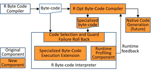
Figure 3.3 shows the diagram of the architecture of ORBIT VM. It is an extension to the GNU R interpreter. It does a lightweight type profiling the first time a function’s byte-code is executed. The second time the function is executed, ORBIT compiles the original byte-codes into specialized byte-codes with guards. Specialized byte-codes use the extended data representation and are interpreted in a more efficient way. If a guard detects a type speculation failure, the interpreter rolls back to the original data format and byte-code sequence, and uses the meet (union) of the types as a new profile type.
3.3.1
Runtime Type Profiling
Although type inference can be done without runtime type profiling, pure static type inference is complex and not sufficiently precise especially in the presence of dynamic attributes like those of R. By only instrumenting a few instructions, ORBIT simplifies the type inference and get a more precise result. The interpretation logic of a few instructions is modified to insert the profiling logic. Table3.1lists these instructions.
Table 3.1: Instrumented R Byte-code instructions in ORBIT
Category Instructions
Load GETVAR,DDVAL,GETVAR MISSOK,DDVAL MISSOK
Function Call CALL,CALLBUILTIN,CALLSPECIAL,ENDASSIGN
Vector Sub-elements Access DFLTSUBSET,DFLTC,DFLTSUBSET2,DOLLAR
The profiler first gets the type of the object on top of the interpreter stack after an instrumented instruction is interpreted, and stores the type into a profiling table indexed with the interpreter’s PC. The type information of a generic R object is stored in three places: thetypein the header, attrib
also in the header to specify the number of dimensions (there is no dim attribute if the number of dimensions is one, i.e. in the case of a vector), andlength in the body section to specify the vector length ofVECTOR. The profiler checks all these attributes, and combines them into a type (see next section) defined by ORBIT. If one instruction is profiled several times (in the same PC location), the final type is the meet of all the types profiled. Because of the R object structure, the type profiling is more complex than other dynamic languages. By carefully design the profiling component, the overhead of profiling is typically less than 10%.
3.3.2
R Optimization Byte-code Compiler and Type Specialized Byte-code
After the profiling information is captured, R optimization byte-code compiler (henceforth referred to as R Opt compiler) use the profiling information to translate the original type generic byte-code into a type specialized byte-code.
The compiler has the following passes
• Decode Translate the binary chunk of the codes into R Opt compiler’s internal byte-code representation.
• Build CFG and stackBuild the control flow graph, and analyze the stack shape before and after each instruction.
• Type inferenceAnalyze each object’s type, including objects in stack and variables defined in the symbol table.
• OptimizationsA few optimization passes that do the real code specialization and byte-code rewriting.
• Redundant cleanClean redundant instructions (Scalar Value Cache load/store, and invalida-tion).
• PC RecalculationCalculate the new PC value for each byte-code instruction. • Reset Jump PCSet the jump target values of the control flow related instructions.
• EncodeTranslate the R Opt compiler’s internal byte-code representation back into the binary format of the R byte-codes.
TheDecode,Build CFG and stack, PC Recalculation,Reset Jump PCandEncodepasses fol-low the standard algorithms described in [21]. The techniques used for other passes are described following.
The type specialized byte-codes include about 140 byte-codes as supplemental to the original R byte-code interpreter’s 90 type generic byte-codes. These byte-codes are formatted and encoded in the same way as the original byte-codes. The R Opt compiler just performs byte-code replace-ment. If the type is known, and an optimization is identified, the original type generic byte-code is replaced by the type specialized byte-code. Otherwise, the original byte-code is remained. This design leads to a fast transformation and the best possible compatibility to the original byte-code interpreter. A detail list of the type specialized byte-codes could be found in the ORBIT source code.
3.3.3
Type Inference
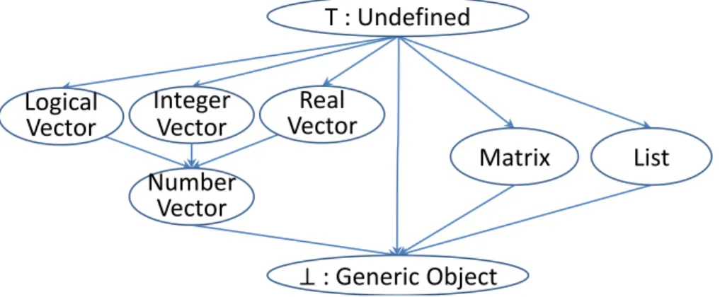
A new simple type lattice system of R is defined here for the type inference, shown in Figure3.4. All vector types have two components, base type (logical, integer, real, etc.) and the length.
The initial type information comes from the type profiling and the constant objects’ type. The initial type of a stack operand generated by a profiled instructions is set to the profiled type. If
T : Undefined
⊥ : Generic Object
Matrix List Logical
Vector Integer Vector Vector Real Number
Vector
Figure 3.4: The type system of ORBIT.
there is no profiling result (the path is not executed during the profiling run), the type is set to the bottom type, generic R object. The initial type of a stack operand generated by a load constant instruction is set to the type of the constant. All other types of stack operands and local frame variables are set to the undefined (top) type.
The type inference algorithm used here is the standard data flow based algorithm. The algo-rithm follows the byte-code interpretation order and uses each instruction’s semantics to compute types until all the types are stable. Different to the traditional type inference, all the types that rely on profiling are marked as speculated types. All the specialized instructions that use speculated types contain a guard to do the check.
3.3.4
Object Representation Specialization
In order to efficiently represent a typed R object, specialized data structures are used in the ORBIT VM, including 1) a specialized interpreter stack, and 2) the Unboxed Value Cache to hold values in the current local frame.
Stack with Boxed and Unboxed Values
The original R vector type object is always represented as R’s VECTOR object, even if a scalar object. In the specialized ORBIT runtime, scalar numbers (boolean, integer and real) are stored
![Figure 1.1: Software used in data analysis competitions in 2011[45]](https://thumb-us.123doks.com/thumbv2/123dok_us/10110107.2911557/16.918.268.620.125.392/figure-software-used-data-analysis-competitions.webp)