On Rates of Convergence for Stochastic
Optimization Problems Under Non-I.I.D.
Sampling
Tito Homem-de-Mello
Department of Industrial Engineering and Management Sciences
Northwestern University
Evanston, IL 60208-3119, U.S.A.
e-mail:
[email protected]
April 14, 2006
Abstract
In this paper we discuss the issue of solving stochastic optimization problems by means of sample average approximations. Our focus is on rates of convergence of esti-mators of optimal solutions and optimal values with respect to the sample size. This is a well studied problem in case the samples are independent and identically distrib-uted (i.e., when standard Monte Carlo is used); here, we study the case where that assumption is dropped. Broadly speaking, our results show that, under appropriate as-sumptions, the rates of convergence forpointwise estimators under a sampling scheme carry over to the optimization case, in the sense that convergence of approximating optimal solutions and optimal values to their true counterparts has the same rates as in pointwise estimation.
Our motivation for the study arises from two types of sampling methods that have been widely used in the Statistics literature. One is Latin Hypercube Sampling (LHS), a stratified sampling method originally proposed in the seventies by McKay, Beckman, and Conover (1979). The other is the class of quasi-Monte Carlo (QMC) methods, which have become popular especially after the work of Niederreiter (1992). The advantage of such methods is that they typically yield pointwise estimators which not only have lower variance than standard Monte Carlo but also possess better rates of convergence. Thus, it is important to study the use of these techniques in sampling-based optimization. The novelty of our work arises from the fact that, while there has been some work on the use of variance reduction techniques and QMC methods in stochastic optimization, none of the existing work — to the best of our knowledge — has provided a theoretical study on the effect of these techniques on rates of convergence for the optimization problem. We present numerical results for some two-stage stochastic programs from the literature to illustrate the discussed ideas.
Key words: Stochastic optimization, two-stage stochastic programming with recourse, Monte Carlo simulation, variance reduction techniques, quasi-Monte Carlo methods, Latin Hypercube sampling.
1
Introduction
In this paper we consider stochastic optimization problems of the form min
x∈X {g(x) := IE[G(x,ξ)]}, (1.1) whereX is a subset of Rn,ξ is a random vector inRs and G:Rn×Rs ½Ris a real valued measurable function. We refer to (1.1) as the “true” optimization problem. The class of problems falling into the framework of (1.1) is quite large, and includes two-stage stochastic programs as a particular instance.
Oftentimes the expectation in (1.1) cannot be calculated exactly, particularly when G
does not have a closed form. In those cases, approximations based on sampling are usually the alternative. One such approximation can be constructed as follows. Consider a family
{gˆN(·)}of random approximations of the function g(·), each ˆgN(·) being defined as ˆ gN(x) := 1 N N X j=1 G(x,ξj), (1.2)
where {ξ1, . . . ,ξN} is a sample from the distribution of ξ. When ξ1, . . . ,ξN — viewed as random variables — are independent and identically distributed (i.i.d.) the quantity ˆgN(x) is called a (standard) Monte Carlo estimator of g(x).
Given the family of estimators{gˆN(·)}defined in (1.2), one can construct the correspond-ing approximatcorrespond-ing program
min
x∈X ˆgN(x). (1.3)
Let ˆxN and ˆνN denote respectively an optimal solution and the optimal value of (1.3). Then, ˆ
xN and ˆνN provide approximations respectively to an optimal solution x∗ and the optimal value ν∗ of the true problem (1.1). Note that the optimization in (1.3) is performed for a fixed sample; for that reason, this is called anexternal sampling approach. When ˆgN(·) is a standard Monte Carlo estimator ofg(·), such an approach is found in the literature under the names of sample average approximation method, stochastic counterpart, and sample-path optimization, among others.
The external sampling approach with standard Monte Carlo has been implemented in various settings, see for instance G¨urkan, ¨Ozge, and Robinson (1999), Kleywegt, Shapiro, and Homem-de-Mello (2001), Plambeck, Fu, Robinson, and Suri (1996). One advantage of that approach lies in its nice convergence properties; for example, it is possible to show that, when
x∗ is the unique optimal solution, ˆx
N → x∗ and ˆνN → ν∗ under fairly general assumptions (see, e.g., Dupaˇcov´a and Wets, 1988, King and Rockafellar, 1993, Robinson, 1996, Shapiro, 1991, 1993). Two properties have proven particulary useful in terms of establishing rates of convergence: the first establish that, under proper conditions, P(|g(ˆxN)−g(x∗)| ≤ ε) and P(kxˆN −x∗k ≤ε) converge to oneexponentially fast in the sample size N for any fixed
ε >0 (Dai, Chen, and Birge, 2000, Kaniovski, King, and Wets, 1995). Under some further conditions one can say more, namely, thatP(ˆxN =x∗) converges to one exponentially fast in the sample size N (Shapiro and Homem-de-Mello, 2000). Exponential rates of convergence
have interesting consequences in terms of complexity of the underlying problems; see Shapiro (2006) for a discussion.
Another useful property establishes that the sequence of optimal values {νˆN} satisfies a certain kind of Central Limit Theorem (CLT). More specifically, one has
N1/2(ˆνN −ν∗) →d Normal(0, σ∗),
where “→d ” denotes convergence in distribution and σ∗ := Var[G(x∗)] (Shapiro, 1991). An immediate conclusion from the above result is that the rate of convergence of optimal values of (1.3) is of order N−1/2. A compilation of these and other related results can be found in Shapiro (2003).
It is no surprise that the sequence of approximating optimal values converges at rate
N−1/2. Indeed, consider the estimator ˆg
N defined in (1.2), and fix x ∈ X. Under mild conditions, it follows from the Central Limit Theorem that√N[ˆgN(x)−g(x)]/σ(x) converges in distribution to the standard Normal, where σ2(x) is the variance of G(x). This implies that the error ˆgN(x)−g(x) converges to zero at the rate N−1/2. That is, even the pointwise estimators converge at rate N−1/2. In many practical cases, the value of N necessary to obtain a reasonable small error under this scheme becomes prohibitively large, especially if evaluation of G(x,ξ) for a given ξ is computationally expensive. This motivates the use of variance reduction techniques that can yield estimators with smaller variance than the ones obtained with standard sampling. Consequently, the same error can be obtained with less computational effort, which is a crucial step for the use of sampling-based methods in large-scale problems.
Several variance reduction techniques have been developed in the Simulation and Statis-tics literature, notably importance sampling, control variates, stratified sampling, and others (see, e.g., Bratley, Fox, and Schrage, 1987, Fishman, 1997, Law and Kelton, 2000). How-ever, incorporation of these techniques into a stochastic optimization algorithm is still at an early stage. Existing work (Bailey, Jensen, and Morton, 1999, Dantzig and Glynn, 1990, Emsermann and Simon, 2000, Higle, 1998, Infanger, 1994, Shapiro and Homem-de-Mello, 1998) already shows that significant benefits can be gained by implementing some of these methods, but these papers only provide empirical evidence of the gain.
Another approach to obtain better pointwise estimators is to choose the sample points in an appropriate manner. Such is the case ofquasi-Monte Carlo methods (QMC); see Niederre-iter 1992 for a comprehensive discussion, and the brief review we provide in section 3.2. This class of methods has been gaining popularity in the past few years, as it has been observed that these techniques can provide rates of convergence for pointwise estimators superior to the N−1/2 obtained with standard Monte Carlo.
A few papers study the optimization problem minx∈XgˆN(x) under QMC: Kalagnanam and Diwekar (1997) provide empirical results for the use of Hammersley sequences (one form of QMC) in stochastic optimization problems; Koivu (2005), Pennanen and Koivu (2005) and Pennanen (2005) show that, under mild assumptions, the estimator function ˆgN con-structed with QMC pointsepiconverges to the true functiong, which guarantees convergence with probability one of optimal values and optimal solutions. Their numerical results also suggest considerable gains in terms of rates of convergence when using QMC methods. Pflug (2004) studies a different type of QMC whereby the sampling points are chosen in a way
to minimize the so-called Wasserstein distance between the original distribution and the empirical distribution generated by the points. Again, the numerical results in Pflug (2004) suggest considerable advantage over standard Monte Carlo.
The above discussion shows that, while there has been some work on the use of variance reduction techniques and QMC methods in stochastic optimization, none of these papers has provided a theoretical study on the effect of these techniques on rates of convergence. The reason is that, without the i.i.d. assumption, many of the classical results in probability theory cannot be applied. One exception is the work of Dai et al. (2000), who provide results on exponential rate of convergence of optimal solutions even without the i.i.d. assumption. However, that paper does not focus on any particular sampling technique; rather, they assume that certain conditions that allow for the application of the Gartner-Ellis Theorem in large deviations theory (see, e.g., Dembo and Zeitouni 1998) are satisfied.
In this paper we propose a study of rates of convergence for optimal solutions and optimal values of the approximating problem (1.3) without imposing that the sample be independent or identically distributed. Our basic requirement is that ˆgN(x)→g(x) with probability one for all x, although we shall impose other conditions as we proceed. More specifically, we show that (i) if the proposed sampling scheme yields exponential rate of convergence for
pointwise estimators, then the convergence ofoptimal solutions will also have an exponential rate, and (ii) if the proposed sampling scheme yields a CLT for pointwise estimators, then the convergence ofoptimal values will obey the CLT as well. The setting is fairly general — i.e. the decision space can be continuous or discrete, and the distributions of the underlying random variables can be continuous or discrete, although some the results will not be valid in some of these cases.
We illustrate the ideas for the particular cases of Latin Hypercube Sampling (LHS) and a specific variation of randomized QMC called scrambled (t, m, s)-nets. We show that, for a particular class of functions, the exponential feature of the rate of convergence is preserved under LHS for pointwise estimators and therefore for estimators of optimal solutions. We also use CLT-type results available for LHS and randomized QMC to illustrate the conver-gence results for estimators of optimal values. In particular, we show that, under LHS, the estimators ˆνN of optimal values converge at a rate of order N−1/2, the same as standard Monte Carlo; for QMC, under appropriate assumptions the sequence {νˆN} converges at a rate of order [(logbN)s−1/N3]1/2, which asymptotically is much better than N−1/2.
We then apply our results to two-stage stochastic linear programs, and discuss the validity of our assumptions in that context. Numerical results are presented for two problems from the literature to illustrate the ideas.
The remainder of the paper is organized as follows: in section 2 we describe our main results for rates of convergence of estimators of optimal solutions and optimal values. In section 3 we apply these results to Latin Hypercube Sampling and randomized quasi-Monte Carlo. We illustrate the ideas for two-stage stochastic programs in section 4 and present numerical results in section 5. Concluding remarks are presented in section 6.
2
Rates of convergence
We discuss separately the results on rates of convergence for optimal solutions and optimal values. Throughout this paper,S∗ and S
N denote the set of optimal solutions of respectively (1.1) and (1.3). Before we study the two cases, we shall make some general assumptions.
Assumption A1: For each x∈X, ˆgN(x)→g(x) with probability one (denoted w.p.1). Assumption A1 is very natural, as it requires the estimators to beconsistent. In the i.i.d. case, this is just the standard Strong Law of Large Numbers, which holds if IE[|gˆN(x)|]<∞ for each x∈X.
We make now an assumption on the integrandGviewed as a function of its first argument:
Assumption A2: The feasibility set X is compact and there exists a measurable function
L:Rs ½Rsuch thatL(ξ)>0 w.p.1, IE[L(ξ)]<∞and, for almost everyξand allx, y ∈X,
|G(x,ξ)−G(y,ξ)| ≤ L(ξ)kx−yk. (2.1) Clearly, Assumption A2 ensures that the functionG(·,ξ) is continuous for almost everyξ. Moreover, it implies that ˆgN(·) and g(·) are also Lipschitz continuous with constants respec-tively equal to ˆLN :=N−1
PN
j=1L(ξj) and IE[L(ξ)]. From (Hiriart-Urruty and Lemarechal, 1993, Theorem IV.3.1.2), we see that if (i) the feasibility setX is compact and contained in the relative interior of the domain ofG(·,ξ) for almost every ξ, and (ii) G(·,ξ) is convex for almost everyξ, then the existence of L(ξ) in Assumption A2 is assured, so in that case only finiteness of IE[L(ξ)] needs to be checked.
In some cases we will replace Assumption A2 with the following condition:
Assumption A3: Either (i) the feasibility set X is finite, or (ii) X is compact, convex and polyhedral, the functionG(·,ξ) is piecewise linear for every value of ξ, and the distribution of ξ has finite support.
It is worthwhile noticing that, under Assumptions A1 and A2, it is known that (see, e.g., Rubinstein and Shapiro 1993, p.67-70):
(i) ˆgN(x)→g(x) uniformly on X w.p.1.; (ii) ˆνN →ν∗ w.p.1;
(iii) dist(ˆxN, S∗)→0 w.p.1.
It is not difficult to see that the above holds under Assumptions A1 and A3 as well — in fact, in that case the result in (iii) is replaced with (iii)0: ˆx
N ∈S∗ w.p.1 forN large enough (cf. proof of Theorem 2.1).
2.1
Convergence of approximating solutions
We start by making the following probabilistic assumption on the estimators {ˆgN(x)}:
Assumption B1: For each x∈X, there exist a number Cx >0 and a function γx(·) such that γx(0) = 0,γx(z)>0 if z >0, and
That is, the probability that the deviation between ˆgN(x) and g(x) is bigger than δ goes to zero exponentially fast with N. Notice that (2.2) implies that ˆgN(x) converges in probability to g(x), which is also ensured by Assumption A1.
Instead of (2.2), we can impose the following weaker condition.
Assumption B10: For each x ∈ X, there exists a function γx(·) such that γx(0) = 0,
γx(z)>0 ifz >0, and lim sup
N→∞ 1
N logP (|ˆgN(x)−g(x)| ≥δ) ≤ −γx(δ) for all δ >0. (2.3)
Some of our results will be stated assuming B1 holds; alternatively, B10 can be used, though in such cases the corresponding result will be stated in asymptotic form as well.
We study now a sufficient condition for Assumption B1 to hold. The main concept behind it arises from the theory oflarge deviations, a well-studied field. For a thorough exposition of the theory, we refer to any of the classical texts in the area, e.g., Dembo and Zeitouni (1998). We present here a result from Drew and Homem-de-Mello (2005).
Proposition 2.1. Consider the sample ξ1, . . . ,ξN used in (1.2), and define the extended real-valued function φN(x, t) := 1 N log IE £ etNgˆN(x)¤. (2.4)
Suppose that for each x ∈ X these exists an extended real-valued function φ∗
x such that
φN(x,·)≤φ∗x(·) for all N, and assume that φ∗x satisfies the following conditions: (i)φ∗x(0) = 0; (ii) φ∗
x(·) is continuously differentiable and strictly convex on a neighborhood of zero;
and (iii) (φ∗
x)0(0) = g(x). Then, Assumption B1 holds, with the functions γx(·) given by
γx(δ) := min{Ix(g(x)+δ), Ix(g(x)−δ)}(where Ix(z) = supt∈R{tz−φ∗x(t)}) and the constants
Cx being all equal to 2.
A simple setting where the conditions of Proposition 2.1 are satisfied is when the functions
φN(x,·),N = 1,2, . . ., are bounded by the log-moment generating function of some random variable Wx (i.e., φ∗x(t) = log IE[etWx]) such that IE[Wx] =g(x). Clearly, condition (i) holds in that case. Moreover, if there exists a neighborhoodN of zero such that φ∗
x(·) is finite on
N, then it is well known that φ∗
x is infinitely differentiable on N and (iii) holds. In that case, Proposition 1 in Shapiro, Homem-de-Mello, and Kim (2002) ensures thatφ∗
x is strictly convex onN.
Note that when the samples {ξi}are i.i.d. we have
φN(x, t) = 1 N log(IE[e tNˆgN(x)]) = 1 N log({IE[e tG(x, )]}N) = log(IE[etG(x, )]) = logM x(t), where Mx(t) := IE[etG(x, )] is the moment generating function of G(x,ξ) evaluated at t. In that case, of course, we have φN(x, t) = φx∗(t) for all N, and the resulting function Ix in Proposition 2.1 is the rate function associated with G(x,ξ). Inequality (2.2) then yields the well-known Chernoff upper bounds on the deviation probabilities. It is also well-known
(Cram´er’s Theorem) that in that caseγx(δ) is anasymptotically exact rate, in the sense that (2.3) holds with equality.
One important consequence of the above developments is the following: Suppose that the function φ∗
x in Proposition 2.1 is dominated by the log-moment generating function of the random variable G(x,ξ), i.e., φ∗
x(t) ≤ φMCx (t) := log IE[etG(x, )]. This immediately implies that the rate function Ix dominates the rate function associated with the random variable
G(x,ξ), which as seen earlier is the asymptotically exact rate function obtained with i.i.d. (i.e., Monte Carlo) sampling. In other words, if one uses a sampling technique that yields functions φN(x,·) for which one can find φ∗x in Proposition 2.1 such that φ∗x(·) ≤ φMCx (·), then the pointwise convergence rate for this sampling technique — in the sense of (2.2) — is at least as good as the rate obtained with standard Monte Carlo. We will use this basic argument repeatedly in the course of this paper.
Under the above conditions, we have the following result. Recall that ˆxN is an optimal solution of (1.3) and S∗ is the set of optimal solutions of (1.1). Below, dist(z, A) denotes the usual Euclidean distance function between a point z and a set A, i.e., dist(z, A) := infy∈Akz−yk.
Theorem 2.1. Consider problem (1.3), and suppose that Assumptions A1 and B1 hold. 1. Suppose that Assumption A2 holds, and that the random variable L(ξ) in
Assump-tion A2 satisfies the large deviaAssump-tions condiAssump-tion in AssumpAssump-tion B1 with N−1PN
j=1L(ξj)
and IE[L(ξ)] in the role of respectively gˆN(x) and g(x).
Then, given ε >0, there exist constants K >0 and α >0 such that
P (dist(ˆxN, S∗)≥ε) ≤ Ke−αN for all N ≥1.
2. Suppose that Assumption A3 holds. Then, there exist constants K >0and α >0 such that
P (ˆxN 6∈S∗) ≤ Ke−αN for all N ≥1.
In either case, the constants K and α depend on the random sample used to generate
ˆ
gN(·) only through respectively the constants Cx and the exponent functions γx(·) in (2.2). The proof of Theorem 2.1 will be based on the following lemma:
Lemma 2.1. Suppose that Assumption B1 holds, and that either (i) the set X is finite, or (ii) the conditions in case 1 of Theorem 2.1 hold. Then, for any δ > 0 there exist positive constants A=A(δ) and α=α(δ) such that
P (|ˆgN(x)−g(x)| ≥δ) ≤ Ae−αN, for all x∈X and all N ≥1. (2.5)
Moreover, there exists a positive constant K (also dependent on δ) such that
Proof. When X is finite, we can set α := infx∈Xγx(δ) in (2.2) to show (2.5) (with A := supx∈XCx). But whenX is infinite, in principle we cannot guarantee that such quantity will be strictly positive, so we need a different argument. Letη:=δ/(3IE[L(ξ)] +δ), and denote byB(x, η) the open ball with centerxand radiusη. Let X ={x1, . . . , xr}be a collection of points in X such that X ⊂ ∪r
k=1B(xk, η). Notice that the existence of X is ensured by the compactness ofX.
Consider now an arbitrary pointx∈X. By construction, there exists some xk ∈ X such that kx−xkk< η. Thus, from (2.1) we have that
|gˆN(x)−gˆN(xk)| ≤ 1 N N X j=1 ¯ ¯G(x,ξj)−G(x k,ξj) ¯ ¯ < LˆNη = δ 3 ˆ LN IE[ÃL(ξ)] +δ/3 (2.7) |g(x)−g(xk)| ≤ IE [|G(x,ξ)−G(xk,ξ)|] < IE[ÃL(ξ)]η < δ/3. (2.8) Moreover, by Assumption B1 (applied to both ˆgN(xk) and ˆLN) we have that
P(|gˆN(xk)−g(xk)| ≥δ/3) ≤ Cxk e
−N γxk(δ/3) (2.9)
P(|LˆN −IE[L(ξ)]| ≥δ/3) ≤ CL e−N γL(δ/3), (2.10) whereCLand γL(·) are the quantities given by Assumption B1 when applied to ˆLN. Finally, since |ˆgN(x)−g(x)| ≤ |gˆN(x)−gˆN(xk)|+|ˆgN(xk)−g(xk)|+|g(x)−g(xk)|, it follows that {|ˆgN(x)−g(x)|< δ} ⊇ {|gˆN(x)−gˆN(xk)|< δ/3} ∩ {|gˆN(xk)−g(xk)|< δ/3} ∩ {|g(xk)−g(x)|< δ/3} ⊇ {|LˆN −IE[L(ξ)]|< δ/3} ∩ {|ˆgN(xk)−g(xk)|< δ/3} (2.11) and then from (2.9)-(2.10) we have that
P (|ˆgN(x)−g(x)| ≥δ) ≤ P (|gˆN(xk)−g(xk)| ≥δ/3) +P(|LˆN −IE[L(ξ)]| ≥δ/3) ≤ Cxk e −N γxk(δ/3)+C Le−N γL(δ/3). By taking α := min µ min k=1,... ,r{γxk(δ/3)}, γL(δ/3) ¶ and A:= 2 max µ max k=1,... ,r{Cxk}, CL ¶ , in-equality (2.5) follows.
To show (2.6), notice that from (2.11) we have
P(|ˆgN(x)−g(x)|< δ for all x∈X) ≥ P ³ {|gˆN(xk)−g(xk)|< δ/3, k= 1, . . . , r} ∩ {|LˆN −IE[L(ξ)]|< δ/3} ´ ≥ 1− r X k=1 P (|gˆN(xk)−g(xk)| ≥δ/3)−P(|LˆN −IE[L(ξ)]| ≥δ/3), (2.12)
where the last inequality stems from a direct application of Bonferroni’s inequality. It follows from (2.9), (2.10) and (2.12) that
P (|gˆN(x)−g(x)|< δ for all x∈X) ≥ 1−
r+ 1 2 Ae
−αN.
The proof of (2.6) whenX is finite follows a very similar argument and is therefore omitted. We return now to the proof of Theorem 2.1.
Proof. Consider first the setting of case 1 of the theorem. Let ε >0 be given. As mentioned earlier, Assumption A2 implies the existence of some δ > 0 such that dist(ˆxN, S∗) < ε whenever |ˆgN(x)−g(x)|< δ for all x∈X; see, e.g., (Rubinstein and Shapiro, 1993, p. 69) for a proof.
Next, suppose that X is finite. Let δ be defined as (1/2) minx∈X\S∗g(x) − ν∗. By
Assumption A1, it is clear that, if |gˆN(x)−g(x)| < δ for all x ∈ X, we have that ˆgN(x) < ˆ
gN(y) for all x ∈S∗ and all y ∈X\S∗, i.e., ˆxN ∈ S∗. Now suppose that the conditions in part (ii) of Assumption A3 hold. Then, from Lemma 2.4 in Shapiro and Homem-de-Mello (2000) we know that there exists a finite set of points {x1, . . . , x`} ∪ {y1, . . . , yq} such that
xi ∈S∗,yj ∈X\S∗ and, if ˆgN(xi)<gˆN(yj) for alli∈ {1, . . . , `}and allj ∈ {1, . . . , q}, then ˆ
xN ∈S∗ (in fact, the set SN forms a face of S∗). Therefore, we can use the same argument as in the case where X is finite. We remark that similar results were derived in Kleywegt et al. (2001) and Shapiro and Homem-de-Mello (2000) in the i.i.d. context.
In either case, by Lemma 2.1 the event {|gˆN(x)−g(x)| < δ for all x ∈ X} occurs with probability at least 1−Ke−αN (where both K and α depend on δ). It follows that in case 1 we have
P(dist(ˆxN, S∗)≥ε) ≤ Ke−αN whereas in case 2 we have
P (ˆxN 6∈S∗) ≤ Ke−αN,
as asserted. Notice that in either case δ does not depend on the particular approximation ˆ
gN(·); therefore, the constants K and α depend on ˆgN(·) only through respectively the constantsCx and the exponent functionsγx(·) in Assumption B1.
In essence, Theorem 2.1 says that the existence of an exponential rate of convergence forpointwise estimators is enough to ensure an exponential rate of convergence for optimal solutions of the corresponding approximating problems, regardless of the sampling scheme adopted. Although reasonably intuitive, such result had not — to the best of our knowledge — been stated or proved anywhere in the literature.
It is important to remark that the last assertion of Theorem 2.1 suggests that a better pointwise convergence rate leads to a better rate of convergence of optimal solutions. Indeed, suppose one has at hand two families of approximations, say, {g¯N(x)} and {g˜N(x)}, whose respective exponent functions ¯γx(·) and ˜γx(·) in (2.2) are such that ¯γx(·)≥˜γx(·) for allx∈X.
Then, the corresponding constants ¯α and ˜αwill be such that ¯α≥α˜, whichsuggests that the family{g¯N(·)} yields a better rate of convergence of ˆxN toS∗. Of course, Theorem 2.1 only gives an upper bound on the deviation probabilities P(ˆxN 6∈S∗) and P (dist(ˆxN, S∗)≥ε), so no definitive statements can be made.
Nevertheless, we shall see later specific situations where the pointwise rate of convergence yields an asymptotically exact rate of convergence for the optimization problem; in those cases, superiority of one sampling scheme over another can be established.
An analogous form of Theorem 2.1 can be derived in case Assumption B10 holds instead of B1. We state the result below for completeness; the proof follows very similar steps to the proof of Theorem 2.1 and is therefore omitted.
Theorem 2.2. Consider problem (1.3), and suppose that Assumptions A1 and B10 hold.
1. Suppose that Assumption A2 holds, and that the random variable L(ξ) in Assump-tion A2 satisfies the large deviaAssump-tions condiAssump-tion in AssumpAssump-tion B10 withN−1PN
j=1L(ξj)
and IE[L(ξ)] in the role of respectively gˆN(x) and g(x).
Then, given ε >0, there exist a constant α >0 such that
lim sup N→∞
1
N logP (dist(ˆxN, S
∗)≥ε) ≤ −α. (2.13)
2. Suppose that Assumption A3 holds. Then, there exists a constant α >0 such that
lim sup N→∞
1
N logP (ˆxN 6∈S
∗) ≤ −α. (2.14)
2.2
Convergence of approximating values
We consider now the convergence of the optimal value of (1.3). In the previous section we showed that a exponential rate of convergence for pointwise estimators leads to an expo-nential rete of convergence for solutions of (1.3); here, we will show that, in the context of Assumption A3, a Central Limit Theorem-type result for pointwise estimators leads to a Central Limit Theorem-type result for the optimal value of (1.3). Outside of the context of A3, however, one needs more than CLT for pointwise estimators.
We start by making the following probabilistic assumptions on the estimators {ˆgN(x)}:
Assumption B2: For each x∈S∗, the random variable W
N(x) defined as WN(x) := ˆ gN(x)−g(x) σN(x) , (2.15) where σ2
N(x) := Var[ˆgN(x)], is such that WN(x) converges in distribution to a standard Normal (denoted WN(x)→d Normal(0,1)).
Of course, Assumption B2 holds in case of i.i.d. sampling under very mild assump-tions — in that case it corresponds to the classical Central Limit Theorem (with σN(x) =
p
Var[G(x,ξ)]/N). However, as we shall see later, B2 holds in other contexts as well. Note that we impose Assumption B2 only on the setS∗ of optimal solutions to (1.1).
The lemma below states a property that will be used in the sequel. In the lemma, the statement “w.p.1 for N large enough” means that, with probability one, there exists anN0 such that, on each sample path of the underlying process, the condition holds for allN > N0. The value of such N0 depends on the particular sample path.
Lemma 2.2. Suppose Assumptions A1 and A3 hold. Then,
ˆ
gN(ˆxN)− min x∗∈S∗gˆN(x
∗) = 0 w.p.1 for N large enough.
Proof. We have already seen in the proof of Theorem 2.1 that, under Assumptions A1 and A3, we have that ˆxN ∈S∗ w.p.1 forN large enough. Consider now an arbitrary sample path where such a condition holds. Then, there existsN0 such that ˆxN ∈S∗ for allN > N0. That is, for each N > N0 there exists some point x∗(N)∈ S∗ such that ˆxN = x∗(N). It follows that
ˆ
gN(ˆxN)−ˆgN(x∗(N)) = 0 for all N > N0.
By definition, ˆxN minimizes ˆgN(·) over X. Together with above equality, this implies that ˆ gN(ˆxN) ≤ min x∗∈S∗gˆN(x ∗) ≤ gˆ N(x∗(N)) = ˆgN(ˆxN) for all N > N0 and hence ˆ gN(ˆxN)− min x∗∈S∗gˆN(x ∗) = 0 for all N > N 0. We then have the following result for rates of convergence:
Theorem 2.3. Consider problem (1.3), and suppose that Assumptions A1 and A3 hold. Suppose also that the estimators ˆgN(x) have the same variance on the set S∗ of optimal
solutions to (1.1), i.e., the function σ2
N(·) is constant on S∗, and let (σ∗N)2 denote that
common value. Then,
ˆ νN −ν∗ σ∗ N − min x∗∈S∗WN(x ∗) d → 0. (2.16)
If, in addition, Assumption B2 holds and problem (1.1) has a unique optimal solution (call it x∗), then ˆ νN −ν∗ σN(x∗) d → Normal(0,1). (2.17)
Proof. By Lemma 2.2 we have that ˆ gN(ˆxN)−ν∗ σ∗ N − minx∗∈S∗gˆN(x∗)−ν∗ σ∗ N
= 0 w.p.1 forN large enough. Since convergence w.p.1 implies convergence in distribution, it follows that
ˆ gN(ˆxN)−ν∗ σ∗ N − minx∗∈S∗gˆN(x ∗)−ν∗ σ∗ N d → 0,
and hence ˆ gN(ˆxN)−ν∗ σ∗ N − min x∗∈S∗ ˆ gN(x∗)−ν∗ σ∗ N d → 0.
Note that the term inside the min operation is actually WN(x∗). Moreover, by definition ˆ
gN(ˆxN) = ˆνN, which then shows (2.16).
Suppose now that B2 holds and that S∗ = {x∗}. Then, since W
N(x∗) →d Normal(0,1), using a classical result in convergence of distributions (see, e.g., Billingsley 1995, Theorem 25.4) we conclude that ˆ νN −ν∗ σN(x∗) d → Normal(0,1).
The above result can be slightly strengthened in case the set S∗ is finite (say, S∗ =
{x1, . . . , x`}) and a multivariate version of Assumption B2 holds — namely, that for some deterministic sequence {τN} such that τN → ∞ the multivariate process τN(ˆgN(x1) −
g(x1), . . . ,ˆg
N(x`) −g(x`)) converges in distribution to a random vector Y with Normal distribution with mean vector zero and covariance matrix Σ. In that case, using a very simi-lar argument to that used by Kleywegt et al. (2001), one can show directly thatτN(ˆνN−ν∗) converges in distribution to minx∗∈S∗Y(x∗). We chose to present our result in the above
form because it only requires a univariate CLT.
As mentioned earlier, outside the context of Assumption A3 stronger conditions are required. One possibility is to assume that Assumption A2 holds and that a version of Assumption B2 for functional spaces holds for the spaceC(X) of continuous functions defined onX. As discussed in Shapiro (1991), Assumption A2 suffices to ensure that eachG(·,ξ) is a random element of the spaceC(X), and hence ˆgN(·) :=N−1
PN
j=1G(·,ξ) is also a random element of C(X). The validity of a CLT in that functional space, in turn, implies that a convergence result such as (2.17) holds. This approach works well in the i.i.d. context, see Shapiro (1991) for a discussion. However, we are not aware of other contexts where a CLT in a functional space exists, so we do not elaborate further on this topic.
3
Applications
3.1
Latin Hypercube Sampling
Stratified sampling techniques have been used in Statistics and Simulation for years (see Bratley et al. (1987) and Fishman (1997) for references). Generally speaking, the idea is to partition the sample space and fix the number of samples on each partition, which should be proportional to the probability of the partition. This way we ensure that the number of sampled points on each region will be approximately equal to theexpected number of points to fall in that region. It is intuitive that such procedure yields better variance than crude Monte Carlo; for proofs, see e.g. Fishman (1997). Notice however that, though theoretically appealing, implementing such procedure is far from trivial, since the difficulty is to determine the partitions as well as to compute the corresponding probabilities.
There are many variants of this basic method, one of the most well-known being the so-called Latin Hypercube Sampling (LHS), introduced by McKay et al. (1979). The LHS method operates as follows: suppose we want to draw N samples from a random vector ξ
with s independent components ξ1, . . . , ξs, each of which has a Uniform(0,1) distribution. The algorithm consists repeating the two steps below for each dimensionj = 1, . . . , s:
1. Generate Y1 ∼U µ 0, 1 N ¶ , Y2 ∼U µ 1 N, 2 N ¶ , . . . , YN ∼U µ N −1 N ,1 ¶ ; 2. Let ξi
j :=Yπ(i), where π is a random permutation of 1, . . . , N. McKay et al. (1979) show that each sample ξi
j (viewed as a random variable) has the
same distribution asξj, which in turn implies the estimators generated by the LHS method are unbiased. In case of arbitrary distributions, the above procedure is easily modified by drawing the sample as before and applying the inversion method to generate the desired random variates.
McKay et al. (1979) also show that, under some conditions, the LHS method does indeed reduce the variance compared to crude Monte Carlo. Stein (1987) shows that, asymptotically (i.e. as the sample sizeN goes to infinity), LHS is never worse than crude Monte Carlo, even without the assumptions of McKay et al. (1979). More specifically, Owen (1998) shows that
VLHS ≤N/(N−1)VM C, where VLHS and VM C are respectively the variances under LHS and crude Monte Carlo.
3.1.1 Exponential rate of convergence
In what follows we assume that the components of the random vector ξ are independent. Suppose now the objective functiong(·) in (1.1) is approximated by a sample average calcu-lated using the LHS method, i.e., for eachi= 1, . . . , s,ξ1
i, . . . , ξiN are samples of ξi (the ith component of ξ) constructed using the LHS method. Call the resulting estimator in (1.2) ˆ
gLHS
N (x). To study convergence properties of the approximating problem in (1.3), we shall use the tools of section 2. Our goal is to show that the family{gˆLHS
N (·)}satisfies assumption B1, so that we can apply Theorem 2.1 to ensure exponential rate of convergence.
We shall restrict our attention to functions satisfying the following assumption.
Assumption C1: For each x ∈ X, the function G(x,·) is monotone in each component. That is, for eachi= 1, . . . , sand each δ >0 we have
either G(x, z+δei) ≥ G(x, z) for all z ∈Rs (3.1) or G(x, z+δei) ≤ G(x, z) for all z ∈Rs, (3.2) where as customaryei denotes the vector with 1 in the ith component and zeros otherwise.
An important case where such an assumption is satisfied is that of two-stage stochastic linear programs with fixed recourse. In section 4 we discuss that case in detail.
Assumption C10: For eachx∈X, the functionG(x,·) is separable in its components, i.e., there exist functions G1, . . . , Gs (all of them mapping Rn ×R to R) such that G(x,ξ) =
G1(x, ξ1) +. . .+Gs(x, ξs). Moreover, |IE[Gj(x, ξj)]|<∞,G(x,·) has at most a finite number of singularities, and the set of points at whichG(x,·) is discontinuous has Lebesgue measure zero.
The importance of Assumptions C1 and C10 in the present context is given by the results below:
Theorem 3.1. Suppose that (i)Assumption C1 holds, and (ii) for each x∈X, the moment generating function of G(x,ξ)(denoted φMC
x (t) := IE[etG(x, )]) is finite everywhere. Consider
the LHS estimators ˆgLHS
N (·) above defined and the corresponding problem minx∈XgˆNLHS(x).
Let xˆLHS
N denote an optimal solution of that problem. Then,
1. If Assumption A2 holds, then given ε >0there exists constants K >˜ 0and α >˜ 0 such that
P¡dist(ˆxLHS
N , S∗)≥ε
¢
≤ Ke˜ −αN˜ for all N ≥1. (3.3)
2. If Assumption A3 holds, then there exist a constant α >˜ 0 such that
P ¡xˆLHS
N 6∈S∗
¢
≤ Ke˜ −αN˜ for all N ≥1. (3.4)
Moreover, in either case the exponentα˜ is at least as large as the corresponding exponent obtained for standard Monte Carlo.
Proof. Note initially that condition (ii) implies that IE[G(x,ξ)2] < ∞ and hence Assump-tion A1 holds under LHS (see Loh 1996). Let φN(x, t) := N1 log IE
h
etNˆgLHS
N (x)
i
. If conditions (i) and (ii) above hold, then by Proposition 6 in Drew and Homem-de-Mello (2005) we have that φN(x, t) ≤ φMCx (t) for all x and all t and hence it follows from Proposition 2.1 that Assumption B1 holds for {gˆLHS
N (·)}. The two cases of the theorem then parallel the two cases of Theorem 2.1, which shows (3.3) and (3.4).
The last assertion of the theorem is a consequence of the remark following the proof of Theorem 2.1. Indeed, the arguments in the previous paragraph show that the constantsCx and the exponent functions γx(·) in (2.2) are the same for both LHS and standard Monte Carlo.
Although Theorem 3.1 only guarantees the same bounds for both LHS and standard Monte Carlo, a closer look at the proof of the inequality φN(x,·)≤ φMCx (·) shows that this inequality tends to be strict and hence LHS tends to behave better than Monte Carlo.
In case Assumption C10 holds instead of C1, we have the following stronger result:
Theorem 3.2. Suppose that the assumptions of Theorem 3.1 are satisfied, but Assumption C10 holds instead of C1. Then, the conclusions of Theorem 3.1 hold. In addition, we have
1. If Assumption A2 holds, then
lim N→∞ 1 N logP ¡ dist(ˆxLHS N , S∗)≥ε ¢ = −∞. (3.5)
2. If Assumption A3 holds, then lim N→∞ 1 N logP ¡ ˆ xLHSN 6∈S∗¢ = −∞. (3.6)
Proof. The proof of the first part of the theorem follows the same steps as the proof of Theorem 3.1 (except that Proposition 4 in Drew and Homem-de-Mello (2005) is invoked instead of Proposition 6).
To show the second part, consider the inverse of the cumulative distribution function Fj of ξj, defined as Fj−1(u) := inf{y ∈ Ξj : Fj(y) ≥ u}, where Ξj denotes the support of the distributionFj. Then, by writing each random variableξj asFj−1(Uj) (where Uj ∼U(0,1)), we have that conditions (i) and (ii) of Theorem 3.1 ensure that the assumptions of Theorem 2 in Drew and Homem-de-Mello (2005) are satisfied. The latter result, in turn, ensures that Assumption B10 holds with the function γ
x =∞everywhere except at zero, where it is equal to zero. Then, (3.5) and (3.6) follow from (2.13) and (2.14) in Theorem 2.2.
The strength of Theorem 3.2, of course, lies in the asymptotic results (3.5)-(3.6), which show that in the separable case the rate of convergence under LHS is superexponential.
3.1.2 Central Limit Theorem
We study now the convergence of optimal values of the approximating problem (1.3) under LHS. To do so we shall apply results of section 2.2. Before that, however, we need to review some results related to the ANOVA decomposition of a function.
Let U = (U1, . . . , Us) be an s-dimensional random vector with uniform distribution on [0,1]s, f : [0,1]s −→ R an arbitrary function and consider the problem of estimating
I := IE[f(U)]. Stein (1987) shows that, when IE[(f(U))2]<∞, f can be decomposed as
f(U) = IE[f(U)] + s
X
k=1
fk(Uk) +r(U), (3.7) where fk(Uk) = IE[f(U)|Uk] − IE[f(U)] and r(U) is the residual term, which satisfies IE[r(U)|Uj] = 0 for all j. Moreover, Stein (1987) also shows that the variance of the estimator ILHS (defined as ILHS := N−1
PN
i=1f(Ui), where U1, . . . , UN are samples drawn with LHS) satisfies σ2 N := Var[ILHS] = N−1IE £ (r(U))2¤+o(N−1) (3.8) asN goes to infinity.
Using the results in (3.7) and (3.8), Owen (1992) shows that, when f is bounded, a Central Limit Theorem holds for the estimatorILHSunder Latin Hypercube Sampling. More specifically, he shows that
N1/2(I
LHS−I) →d Normal(0, σ2), whereσ2 := IE[(r(U))2]. (3.9) Next, notice that from (3.8) we can write
ILHS−I σN = hN1/2(ILHS−I) σ2+o(N−1) N−1 i1/2.
Since N1/2(I
LHS −I) →d Normal(0, σ2) and the deterministic sequence {[σ2 + o(N
−1)
N−1 ]1/2}
converges toσ, it follows from a classical result in probability theory (see, e.g., Chung 1974, p. 93) that, whenσ >0, ILHS−I σN d → 1 σNormal(0, σ 2) = Normal(0,1). (3.10)
Notice that the condition IE[(f(U))2] < ∞ also implies that a Strong Law of Large Numbers holds for LHS, i.e.,
|ILHS−I| → 0 w.p.1; (3.11)
for a proof, see Loh (1996).
By applying (3.10) to our setting we see that Assumption B2 holds for LHS under some boundedness condition, provided that the ANOVA residual of G(x,·) is positive for all x ∈ S∗. Moreover, the same boundedness condition implies, via (3.11), that Assumption A1 holds. Thus, under additional assumptions we can apply Theorem 2.3. As before, we write
ξ = (F1−1(U1), . . . , Fs−1(Us)), where U1, . . . , Us are independent uniform random variables in [0,1]. We summarize the result in the theorem below.
Theorem 3.3. Consider the LHS estimators gˆLHS
N (·) above defined and the corresponding
problem minx∈XgˆNLHS(x). Let xˆLHSN and νˆNLHS denote respectively an optimal solution and the
optimal value of that problem.
1. If Assumption A2 holds, then dist(ˆxLHS
N , S∗)→0 w.p.1 and νˆNLHS→ν∗ w.p.1.
2. If Assumption A3 holds, then xˆLHS
N ∈ S∗ w.p.1 for N large enough and νˆNLHS → ν∗
w.p.1. In addition, suppose that for each x ∈ X the function G(x,·) is bounded and that the distribution of ξ has bounded support. If problem (1.1) has a unique optimal solution (call it x∗) and the function G(x∗,·) is not separable in its components, then
ˆ νN −ν∗ σN(x∗) d → Normal(0,1), where σ2
N(x∗)is the variance of ˆgNLHS(x∗). Moreover, there exists a positive constant C
such that
σ2
N(x∗) = N−1C+o(N−1) (3.12)
as N → ∞.
Theorem 3.3 shows that the rate of convergence of optimal values under LHS (under the conditions of Assumption A3) is N−1/2. Thus, compared to standard Monte Carlo we can see that, although LHS will likely reduce the variance of pointwise estimators, it cannot improve the rate of convergence unless the functionG(x∗,·) is separable in its components, since in that case the residual in the ANOVA decomposition of G(x∗,·) is equal to zero and so we expect the convergence rate to be much faster. Indeed, recall from Theorem 3.2 that, under the assumptions of that theorem (which include separability), convergence of optimal solutions is superexponential. Note also that, whenS∗ is finite (but not necessarily a singleton) andG(x∗,·) is not separable in its components for allx∗ ∈S∗, the stronger result discussed in the paragraph following the proof of Theorem 2.3 applies withτN =N1/2, since the aforementioned CLT result proved by Owen (1992) is also valid in a multivariate context.
3.2
Randomized Quasi Monte Carlo
For completeness, we provide in this section a brief review of quasi-Monte Carlo (QMC) techniques. We follow mostly Niederreiter (1992), which we refer to for comprehensive treatments of QMC concepts. Let U be an s-dimensional random vector with uniform distribution on [0,1]s, f : [0,1]s −→ R an arbitrary function and consider the problem of estimatingI := IE[f(U)].
The basic idea of QMC is to calculate a sample average estimate as in the standard Monte Carlo but, instead of drawing a random sample from the uniform distribution on [0,1]s, a certain set of pointsu1, . . . , uN on space [0,1]sis carefully chosen. The deterministic estimate
IQMC:= 1 N N X i=1 f(ui) (3.13)
is constructed. A key result is the so-called Koksma-Hlawka inequality which, roughly speak-ing, states that the quality of the approximation given byIQMCdepends on the quality of the chosen points (measured by the difference between the corresponding empirical measure and the uniform distribution, which is quantified by the so-calledstar-discrepancy) as well as on the nature of the function f (measured by its total variation). A great deal of the research on QMC methods aims at determining ways to construct low-discrepancy sequences, i.e., sequences of pointsu1, u2, . . . for which the star-discrepancy is small for allN. A particular type of sequence that has proven valuable is defined in terms of (t, m, s)-nets. We need some definitions before delving into more details, which we do next.
Let b ≥ 2 be an arbitrary integer, called the base. An elementary interval in base b (in dimension s) is a subinterval E of [0,1]s of the form
E = s Y j=1 · aj bdj, aj + 1 bdj ¸
for nonnegative integers {aj} and {dj} such that aj < bdj for all j. The volume of E is
b−Pjdj. Next, let t and m be nonnegative integers such that t ≤ m. A finite sequence of
bm points is a (t, m, s)-net in base b if every elementary interval in base b of volume bt−m contains exactlybt points of the sequence. A sequence of pointsu1, u2, . . . is a (t, s)-sequence in base b if, for all integersk ≥0 andm > t, the set of points consisting of the un such that
kbm ≤n <(k+ 1)bm is a (t, m, s)-net in baseb.
The advantage of (t, m, s)-nets becomes clear from a result due to (Niederreiter, 1992, Theorems 4.10 and 4.17), who shows that the error|IQMC−I| is: (i) of order (logN)s−1/N when IQMC is computed from a (t, m, s)-net in base b with m >0; (ii) of order (logN)s/N whenIQMC is computed from the first N ≥2 terms of a (t, s)-sequence in base b. Note that in case (i) N must be equal to bm, whereas in case (ii) N is arbitrary, which explains the weaker bound. In either case, it is clear that, asymptotically, the error is smaller thanN−1/2 given by standard Monte Carlo methods.
Despite the advantage of QMC with respect to error rates, the method has two major drawbacks:
(a) The bounds provided by the Koksma-Hlawka inequality involve difficult-to-compute quantities such as the total variation of f, i.e., they yield qualitative (rather than quantitative) results; hence, obtaining an exact estimate of the error may be difficult. (b) A comparison of the functions (logN)s/N and N−1/2 shows that even though asymp-totically the error from QMC is smaller than the error from standard Monte Carlo, such an advantage does not appear until N is very large, unless s is small.
These difficulties have long been realized by the QMC community, and various remedies have been proposed. A common way to overcome difficulty (a) above is to incorporate some ran-domness into the choice of QMC points. By doing so, errors can be estimated using standard methods, e.g., via multiple independent replications. This is the main idea of randomized
QMC methods (RQMC), see Fox (2000) and Owen (2000) for detailed discussions.
One particular technique we are interested in using relies on “scrambling” the decimal digits of each point of a (t, s)-sequence in a proper way. This idea was proposed by Owen (1995), and has gained popularity due to the nice properties of the randomized sequence. We shall use these properties below.
3.2.1 Using QMC in optimization
Consider again the family of estimators defined in (1.2), and assume thatN is of the form
bm for some positive integer m. Suppose that {ξi} is generated by a (t, m, s)-net, and call the resulting family {ˆgNQMC(x)}.
Let us fixx∈X for a moment. As discussed above, when{ξi}is generated by astandard (i.e., not scrambled) (t, m, s)-net we have
|gˆNQMC(x)−g(x)| = O µ (logbN)s−1 N ¶ , (3.14)
provided thatG(x,·) is of finite total variation (in the sense of Hardy and Krause). Clearly, this implies that ˆgNQMC(x) → g(x) as N → ∞. Now suppose that {ξi} is generated by a scrambled (t, m, s)-net, and call the corresponding estimator ˆgRQMCN . Owen (1997a) shows that scrambled (t, m, s)-nets are (t, m, s)-nets with probability one, which then implies that
ˆ
gNRQMC(x)→g(x) w.p.1. (3.15)
Moreover, ˆgRQMCN (x) is an unbiased estimator of g(x), i.e., IE[ˆgNRQMC(x)] =g(x). Notice that the term “with probability one” above refers to the probability space where the random permutations that are part of the scrambling algorithm lie. We assume that this probability space is the same where the random vectorsξ are defined.
For some of the results that follow we will need the following assumption.
Assumption D1: Suppose the following conditions hold for each x∈S∗:
¯ ¯ ¯ ¯ ∂ s ∂u1. . . ∂us G(x, F−1(u1, . . . us))− ∂s ∂u1. . . ∂us G(x, F−1(v1, . . . vs)) ¯ ¯ ¯ ¯ ≤ Bku−vkβ (3.16)
(for someB >0 and some β ∈(0,1]), and Z [0,1]s · ∂s ∂u1. . . ∂us G(x, F−1(u 1, . . . us)) ¸2 du > 0. (3.17) In the above, F−1 is a mapping from ∈ [0,1]s into Rs such that ξ = F−1(U) and U is a random vector uniformly distributed on [0,1]s.
A few remarks about cases where Assumption D1 is satisfied are now in order. Suppose that the components ξ1, . . . , ξs of ξ are mutually independent. As before, we can write
ξ= (F−1
1 (U1), . . . , Fs−1(Us)), whereU1, . . . , Us are independent uniform random variables in [0,1] andF−1
j is the inverse cdf ofξj. Suppose momentarily thatGis infinitely differentiable in the second argument and that eachFj−1 is differentiable as well. Then, we have that
∂ ∂u1 G(x, F−1 1 (u1), . . . , Fs−1(us)) = ∂ ∂ξ1 G(x, ξ1, F2−1(u2). . . , Fs−1(us)) ¯ ¯ ¯ ¯ ξ1=F1−1(u1) ∂ ∂u1 F−1 1 (u1) so by repeating the calculation for the higher-order mixed derivatives we obtain that
H(u1, . . . , us) := ∂s ∂u1. . . ∂us G(x, F−1 1 (u1), . . . , Fs−1(us)) = (3.18) = ∂ s ∂ξ1. . . ∂ξs G(x, ξ1, . . . , ξs) ¯ ¯ ¯ ¯ξj=Fj−1(uj) j=1,... ,s ∂ ∂u1 F−1 1 (u1). . . ∂ ∂us F−1 s (us). (3.19) It follows that, if the gradient of the function H defined in (3.18) is uniformly bounded for allu∈[0,1]s, thenH is Lipschitz (see, e.g, Bartle 1987, Corollary 40.6), i.e., (3.16) holds. A sufficient condition for uniform boundedness of ∇H(u) on [0,1]s is its continuity on [0,1]s. Equation (3.19) shows that continuous differentiability of G (up to order s+ 1) and F−1
j ,
j = 1, . . . , s(up to second order) on the closed set [0,1]ssuffice for that. Of course, imposing a continuous differentiability assumption on F−1
j restricts the type of distributions that can be used; we shall return to that issue shortly.
Condition (3.17) essentially says that interactions of order up tosare significant, at least on a set of positive probability. For example, (3.17) does not hold if G(x,·) is linear for
x∈S∗, since the mixed derivatives of any order bigger than 1 are equal to zero. Situations like that suggest that the effective dimension of the problem is less than s (Owen, 1997a) — indeed, in the linear case the effective dimension is 1. In that case, one should apply quasi-Monte Carlo only to the most significant variables, for which mutual interaction is significant.
Applying the above results on randomized QMC to the general context of section 2.2 we obtain the following:
Theorem 3.4. Consider the RQMC estimators gˆNRQMC(·)above defined and the correspond-ing problemminx∈XgˆRQMCN (x). LetxˆRQMCN andνˆNRQMCdenote respectively an optimal solution
and the optimal value of that problem.
1. If Assumption A2 holds, then dist(ˆxRQMCN , S∗)→0 w.p.1 and ˆνRQMC
2. If Assumption A3 holds, then xˆRQMCN ∈S∗ w.p.1 for N large enough and νˆRQMC
N →ν∗
w.p.1. If, in addition, Assumption D1 holds, problem (1.1) has a unique optimal solution (call it x∗) and the samples {ξi} are generated by a scrambled (0, m, s)-net
(i.e., t = 0), then ˆ νNRQMC−ν∗ σN(x∗) d → Normal(0,1), where σ2
N(x∗)is the variance of ˆgNRQMC(x∗). Moreover, whenN is of the form bm, there
exist positive constants cand C such that
c(logbN)s−1 N3 ≤ σ 2 N(x∗) ≤ C (logbN)s−1 N3 (3.20) as m→ ∞.
Proof. Let us fix x ∈ X. The assertion in case 1 and the first assertion in case 2 follow directly from (3.15) (which implies that Assumption A1 holds) and the remark following Assumption A3.
Consider now the random variable W(x) defined as
W(x) := gˆ RQMC N (x)−g(x) σN(x) , (3.21) where σ2
N(x) := Var[ˆgRQMCN (x)]. Here we resort to a key result on scrambled (t, m, s)-nets proved by Loh (2003) — building upon previous results by Owen (1997a,b) — that says that a Central Limit Theorem holds for pointwise estimators constructed with a scrambled (0, m, s )-net. Assumption D1 essentially translates the conditions in Loh (2003) into our notation. It follows that, under D1, W(x) converges in distribution to the standard normal for each
x∈S∗, i.e., Assumption B2 holds and hence the conclusion follows from Theorem 2.3. Theorem 3.4 shows the benefits of using randomized quasi-Monte Carlo methods in opti-mization. Essentially, it says that, in the setting of Assumption A3, the convergence rate of optimal values is of order [(logbN)s−1/N3]1/2, which asymptotically is much better than the
N−1/2 obtained with standard Monte Carlo. This suggests that RQMC methods can be very efficacious for stochastic optimization. Note however that, strictly speaking, the theorem applies only to the case whereX is finite, since the assumption of finite support of ξ in the second case of Assumption A3 conflicts with the smoothness condition in Assumption D1. We discuss the smoothness issue in more detail next.
Discussion of smoothness
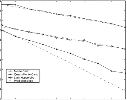
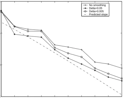
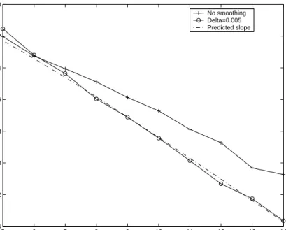
It must be noted that the assumptions of Theorem 3.4 are important to ensure that the convergence rate [(logbN)s−1/N3]1/2 is achieved. In particular, it is important that the smoothness condition required by Assumption D1 hold. Without smoothness, not even pointwise estimation yields such a rate. To illustrate this point, consider the estimation of IE[(Y1Y2Y3)2], where Y1, Y2, Y3 are independent random variables with discrete distribution
![Figure 1: Rates of convergence for pointwise estimation of IE[(Y 1 Y 2 Y 3 ) 2 ].](https://thumb-us.123doks.com/thumbv2/123dok_us/10063441.2906056/21.918.275.690.351.679/figure-rates-convergence-pointwise-estimation-y-y-y.webp)
![Figure 2: Values of the estimates of IE[(Y 1 Y 2 Y 3 ) 2 ].](https://thumb-us.123doks.com/thumbv2/123dok_us/10063441.2906056/22.918.281.692.113.435/figure-values-estimates-y-y-y.webp)