May 2007, Volume 20, Issue 9. http://www.jstatsoft.org/
Extended Rasch Modeling: The
eRm
Package for
the Application of IRT Models in
R
Patrick Mair
Wirtschaftsuniversit¨at Wien
Reinhold Hatzinger
Wirtschaftsuniversit¨at Wien
Abstract
Item response theory models (IRT) are increasingly becoming established in social science research, particularly in the analysis of performance or attitudinal data in psy-chology, education, medicine, marketing and other fields where testing is relevant. We propose theRpackageeRm(extended Rasch modeling) for computing Rasch models and several extensions.
A main characteristic of some IRT models, the Rasch model being the most prominent, concerns the separation of two kinds of parameters, one that describes qualities of the subject under investigation, and the other relates to qualities of the situation under which the response of a subject is observed. Using conditional maximum likelihood (CML) estimation both types of parameters may be estimated independently from each other. IRT models are well suited to cope with dichotomous and polytomous responses, where the response categories may be unordered as well as ordered. The incorporation of linear structures allows for modeling the effects of covariates and enables the analysis of repeated categorical measurements.
TheeRmpackage fits the following models: the Rasch model, the rating scale model (RSM), and the partial credit model (PCM) as well as linear reparameterizations through covariate structures like the linear logistic test model (LLTM), the linear rating scale model (LRSM), and the linear partial credit model (LPCM). We use an unitary, efficient CML approach to estimate the item parameters and their standard errors. Graphical and numeric tools for assessing goodness-of-fit are provided.
Keywords: Rasch model, LLTM, RSM, LRSM, PCM, LPCM, CML estimation.
1. Introduction
Rost (1999) claimed in his article that “even though the Rasch model has been existing for such a long time, 95% of the current tests in psychology are still constructed by using methods
from classical test theory” (p. 140). Basically, he quotes the following reasons why the Rasch model is being rarely used: The Rasch model in its original form (Rasch 1960), which was limited to dichotomous items, is arguably too restrictive for practical testing purposes. Thus, researchers should focus on extended Rasch models. In addition, Rost argues that there is a lack of user-friendly software for the computation of such models. Hence, there is a need for a comprehensive, user-friendly software routine. Corresponding recent discussions can be found inKubinger (2005) and Borsboom(2006).
The focus of this article is on the following Rasch model extensions that can be computed by means of theeRmpackage: the linear logistic test model (Scheiblechner 1972), the rating scale model (Andrich 1978), the linear rating scale model (Fischer and Parzer 1991), the partial credit model (Masters 1982), and the linear partial credit model (Glas and Verhelst 1989;Fischer and Ponocny 1994). These models and their main characteristics are presented in Section2.
Concerning parameter estimation, these models have an important feature in common: Sep-arability of item and person parameters. This implies that the item parameters β can be estimated without estimating the person parameters achieved by conditioning the likelihood on the sufficient person raw score. This conditional maximum likelihood (CML) approach is described in Section3.
Finally, in Section 4, the corresponding implementation in R (R Development Core Team 2006) is described by means of several examples. The eRm package uses a design matrix approach which allows to the user to impose repeated measurement designs as well as group contrasts. By combining these types of contrasts one allows that the item parameter may differ over time with respect to certain subgroups. At this point it is already noted that it is not possible to allow for group contrasts without repeated measurement points since this contradicts to Rasch’s claim for subgroup invariance. Note that it is certainly possible to impose any number of time contrasts time without regarding group differences in order to examine longitudinal hypotheses only. However, to illustrate the flexibility of the eRm package some examples are given to show how suitable design matrices can be constructed.
2. Extended Rasch models
2.1. General expressions
Briefly after the first publication of the basic Rasch Model (Rasch 1960), the author worked on polytomous generalizations which can be found inRasch(1961). Andersen(1995) derived the representations below which are based on Rasch’s general expression for polytomous data. The data matrix is denoted asXwith the persons in the rows and the items in the columns. In total there are v = 1, ..., n persons and i = 1, ..., k items. A single element in the data matrix X is indexed by xvi. Furthermore, each item Ii has a certain number of response categories, denoted by h = 0, ..., mi. The corresponding probability of response h on item i can be derived in terms of the following two expressions (Andersen 1995):
P(Xvi=h) =
exp[φh(θv+βi) +ωh]
Pmi
l=0exp[φl(θv+βi) +ωl]
or P(Xvi=h) = exp[φhθv+βih] Pmi l=0exp[φlθv+βil] . (2)
Here, φh are scoring functions for the item parameters, θv are the uni-dimensional person parameters, andβi are the item parameters. In Equation 1, ωh corresponds to category pa-rameters, whereas in Equation2βih are the item-category parameters. The meaning of these parameters will be discussed in detail below. Within the framework of these two equations, numerous models have been suggested that retain the basic properties of the Rasch model so that CML estimation can be applied.
2.2. Representation of extended Rasch models
For the ordinary Rasch model for dichotomous items, Equation1 reduces to
P(Xvi= 1) =
exp(θv−βi) 1 + exp(θv−βi)
. (3)
The main assumptions, which hold as well for the generalizations presented in this paper, are: uni-dimensionality of the latent trait, sufficiency of the raw score, local independence, and parallel item characteristic curves (ICCs). Corresponding explanations can be found, e.g., in
Fischer(1974) and mathematical derivations and proofs in Fischer(1995a).
For dichotomous items,Scheiblechner(1972) proposed the (even more restricted) linear logis-tic test model (LLTM), later formalized byFischer(1973), by splitting up the item parameters into the linear combination
βi = p
X
j=1
wijηj. (4)
Scheiblechner (1972) explained the dissolving process of items in a test for logics (“Mengen-rechentest”) by so-called “cognitive operations”ηj such as negation, disjunction, conjunction, sequence, intermediate result, permutation, and material. Note that the weightswij for itemi and operationjhave to be fixed a priori. Further elaborations about the cognitive operations can be found in Fischer (1974, p. 361ff.). Thus, from this perspective the LLTM is more parsimonous than the Rasch model.
Though, there exists another way to look at the LLTM: A generalization of the basic Rasch model in terms of repeated measures and group contrasts. It should be noted that both types of reparameterization also apply to the linear rating scale model (LRSM) and the linear partial credit model (LPCM) with respect to the basic rating scale model (RSM) and the partial credit model (PCM) presented below. Concerning the LLTM, the possibility to use it as a generalization of the Rasch model for repeated measurements was already introduced by Fischer (1974). Over the intervening years this suggestion has been further elaborated.
Fischer(1995b) discussed certain design matrices which will be presented in Section 2.3 and on the basis of examples in Section4.
At this point we will focus on a simple polytomous generalization of the Rasch model, the RSM (Andrich 1978), where each itemIimust have the same number of categories. Pertaining
to Equation1, φh may be set to h with h= 0, ..., m. Since in the RSM the number of item categories is constant,m is used instead of mi. Hence, it follows that
P(Xvi =h) =
exp[h(θv+βi) +ωh]
Pm
l=0exp[l(θv+βi) +ωl]
, (5)
withk item parametersβ1, ..., βk andm+ 1 category parametersω0, ..., ωm. This
parameter-ization causes a scoring of the response categories Ch which is constant over the single items. Again, the item parameters can be split up in a linear combination as in Equation 4. This leads to the LRSM proposed byFischer and Parzer(1991).
Finally, the PCM developed byMasters (1982) and its linear extension, the LPCM (Fischer and Ponocny 1994), are presented. The PCM assigns one parameter βih to each Ii ×Ch combination for h = 0, ..., mi. Thus, the constant scoring property must not hold over the items and in addition, the items can have different numbers of response categories denoted by
mi. Therefore, the PCM can be regarded as a generalization of the RSM and the probability for a response of personv on category h (itemi) is defined as
P(Xvih = 1) =
exp[hθv+βih]
Pmi
l=0exp[lθv+βil]
. (6)
It is obvious that (6) is a simplification of (2) in terms ofφh =h. As for the LLTM and the LRSM, the LPCM is defined by reparameterizing the item parameters of the basic model, i.e., βih= p X j=1 wihjηj. (7)
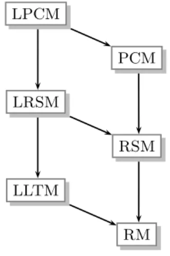
At this point it is important to point out the model hierarchy of these six models (Figure
1). This hierarchy is the base for a unified CML approach presented in the next section. It is outlined again that the linear extension models can be regarded either as generalizations or as more restrictive formulations pertaining to the underlying base model. The hierarchy for the basic model is straightforward: The RM allows only items with two categories, thus each item is represented by one parameterβi. The RSM allows for more than two (ordinal) categories each represented by a category parameter ωh. Due to identifiability issues,ω0 and
ω1 are restricted to 0. Hence, the RM can be seen as a special case of the RSM whereas, the
RSM in turn, is a special case of the PCM. The latter model assigns the parameter βih to each Ii×Ch combination.
To conclude, the most general model is the LPCM. All other models can be considered as simplifications of Equation6combined with Equation7. As a consequence, once an estimation procedure is established for the LPCM, this approach can be used for any of the remaining models. This is what we quote as unified CML approach. The corresponding likelihood equations follow in Section3.
2.3. The concept of virtual items
When operating with longitudinal models, the main research question is whether an individ-ual’s test performance changes over time. The most intuitive way would be to look at the
LPCM PCM LRSM RSM LLTM RM
Figure 1: Model hierarchy
shift in abilityθv across time points. Such models are presented e.g. inMislevy (1985),Glas (1992), and discussed byHoijtink(1995).
Yet there exists another look onto time dependent changes, as presented in Fischer (1995b, p 158ff.): The person parameters are fixed over time and instead of them the item parameters change. The basic idea is that one item Ii is presented at two different times to the same person Sv is regarded as a pair of virtual items. Within the framework of extended Rasch models, any change in θv occuring between the testing occasions can be described without loss of generality as a change of the item parameters, instead of describing change in terms of the person parameter. Thus, with only two measurement points, Ii with the corresponding parameterβi generates two virtual itemsIr and Is with associated item parameters βr∗ and
βs∗. For the first measurement pointβr∗ =βi, whereas for the secondβs∗=βi+τ. In this linear combination theβ∗-parameters are composed additively by means of the real item parameters
β and the treatment effects τ. This concept extends to an arbitrary number of time points or testing occasions.
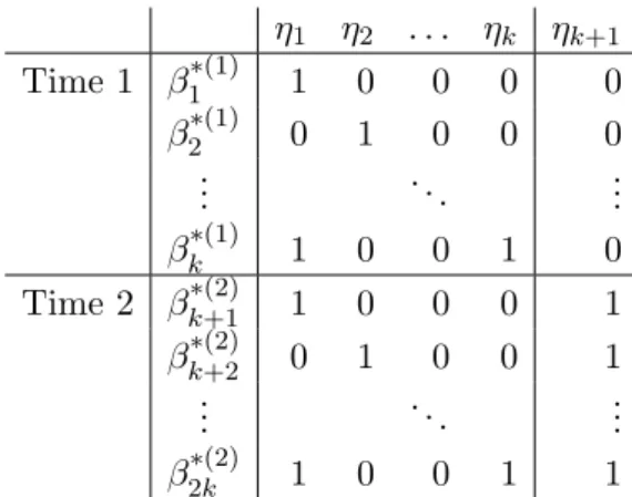
Correspondingly, for each measurement point t we have a vector of virtual item parameters β∗(t)of lengthk. These are linear reparameterizations of the originalβ(t), and thus the CML approach can be used for estimation. In general, for a simple LLTM with two measurement points the design matrix W is of the form as given in Table 1.
The parameter vector β∗(1) represents the item parameters for the first test occasion, β∗(2)
the parameters for the second occasion. It might be of interest whether these vectors differ. The corresponding trend contrast is ηk+1. Due to this contrast, the number of original β
-parameters is doubled by introducing the 2kvirtual item parameters. If we assume a constant shift for all item parameters, it is only necessary to estimate ηb
0
= (bη1, ...,ηbk+1) where ηbk+1
gives the amount of shift. Since according to (4), the vector βb ∗
is just a linear combination ofηb.
As mentioned in the former section, when using models with linear extensions it is possible to impose group contrasts. By doing this, one allows that the item difficulties are different across subgroups. However, this is possible only for models with repeated measurements and virtual items since otherwise the introduction of a group contrast leads to overparameterization and the group effect cannot be estimated by using CML.
η1 η2 . . . ηk ηk+1 Time 1 β1∗(1) 1 0 0 0 0 β2∗(1) 0 1 0 0 0 .. . . .. ... βk∗(1) 1 0 0 1 0 Time 2 βk∗(2)+1 1 0 0 0 1 βk∗(2)+2 0 1 0 0 1 .. . . .. ... β2∗k(2) 1 0 0 1 1
Table 1: A design matrix for an LLTM with two timepoints.
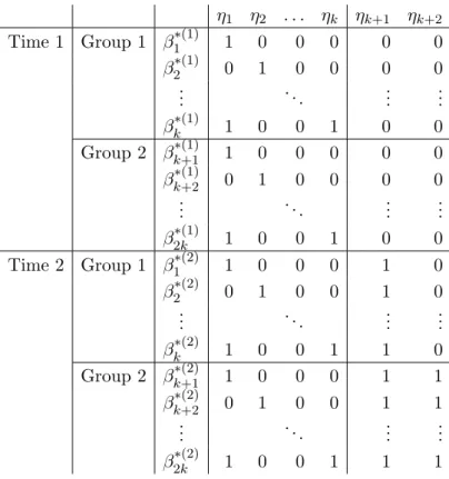
Table2 gives an example for a repeated measurement design where the effect of a treatment is to be evaluated by comparing item difficulties regarding a control and a treatment group. The number of virtual parameters is doubled compared to the model matrix given in Table
1.
Again,ηk+1is the parameter that refers to the time contrast, andηk+2is a group effect within
measurement point 2. More examples are given in Section4and further explanations can be found in Fischer (1995b), Fischer and Ponocny (1994), and in the software manual for the LPCM-Win program byFischer and Ponocny-Seliger (1998).
3. A unified CML approach and model testing
3.1. The likelihood expressionsGenerally, there are several approaches to estimate parameters in IRT models, see, e.g.,Baker and Kim (2004). For Rasch models, the commonly used approaches are either conditional maximum likelihood (CML) or marginal maximum likelihood (MML) estimation which are asymptotically equivalent and provide consistent estimators (Pfanzagl 1994). Using the MML approach, the user has to specify a density function for the person parameters, i.e. f(θ), and if this specification is wrong, MML is inferior to CML. However, there exist also some nonparametric approaches to specify f(θ) (de Leeuw and Verhelst 1986). Furthermore, a pseudo-ML estimation has been proposed as well (Anderson, Li, and Vermunt 2007).
In theeRmpackage, CML is used because, apart from the desirable properties of the estima-tors, it stays close to the concept of specific objectivity (Rasch 1960,1977; Fisher Jr. 1992), proposed by Rasch and well-founded from a epistemological point of view. Furthermore, using the CML approach,LR-tests can be carried out immediately.
The main idea behind the CML estimation is that the person’s raw scorerv = Pki=1xvi is a sufficient statistic. Thus, by conditioning the likelihood onto r0 = (r1, ..., rn), the person
parameters θ, which in this context are nuisance parameters, vanish from the likelihood equation, thus, leading to consistently estimated item parametersβb.
η1 η2 . . . ηk ηk+1 ηk+2 Time 1 Group 1 β1∗(1) 1 0 0 0 0 0 β2∗(1) 0 1 0 0 0 0 .. . . .. ... ... βk∗(1) 1 0 0 1 0 0 Group 2 βk∗(1)+1 1 0 0 0 0 0 βk∗(1)+2 0 1 0 0 0 0 .. . . .. ... ... β2∗(1)k 1 0 0 1 0 0 Time 2 Group 1 β1∗(2) 1 0 0 0 1 0 β2∗(2) 0 1 0 0 1 0 .. . . .. ... ... βk∗(2) 1 0 0 1 1 0 Group 2 βk∗(2)+1 1 0 0 0 1 1 βk∗(2)+2 0 1 0 0 1 1 .. . . .. ... ... β2∗(2)k 1 0 0 1 1 1
Table 2: Design matrix for a repeated measurements design with treatment and control group.
Some restrictions have to be imposed on the parameters to ensure identifiability. This can be achieved, e.g., by setting certain parameters to zero depending on the model. In the Rasch model one item parameter has to be fixed to 0. This parameter may be considered as baseline difficulty. In addition, in the RSM the category parameters ω0 and ω1 are also
constrained to 0. In the PCM all parameters representing the first category, i.e. βi0 with
i= 1, . . . , k, and one additional item-category parameter, e.g., β11 have to be fixed. For the
linear extensions it holds that theβ-parameters that are fixed within a certain condition (e.g. first measurement point, control group etc.) are also constrained in the other conditions (e.g. second measurement point, treatment group etc.).
At this point, for the LPCM the likelihood equations with corresponding first and second order derivatives are presented (i.e. unified CML equations). In the first version of the eRmpackage numerical approximations of the Hessian matrix are used. However, to ensure numerical accuracy and to speed up the estimation process, it is planned to implement the analytical solution as given below.
The conditional log-likelihood equation for the LPCM is
logLc = k X i=1 mi X h=1 x+ih p X j=1 wihjηj− rmax X r=1 nrlogγr. (8)
score is quoted asnr. Alternatively, by going down to an individual level, the last sum overr can be replaced byPn
v=1logγrv. It is straightforward to show that the LPCM as well as the
other extended Rasch models, define an exponential family (Andersen 1983). Thus, the raw scorerv is minimally sufficient forθv and the item totals x.ih are minimally sufficient for βih. Crucial expressions are theγ-terms which are known aselementary symmetric functions. An elaborated derivation of these terms for the ordinary RM can be found in Fischer (1974) and an overview of various computation algorithms is given in Liou(1994). However, in the eRmpackage the numerically stablesummation algorithm as suggested byAndersen(1972) is implemented. Fischer and Ponocny(1994) adopted this algorithm for the LPCM and devised also the first order derivative for computing the corresponding derivative of logLc:
∂logLc ∂ηa = k X i=1 mi X h=1 wiha x+ih−ih rmax X r=1 nr γr(i) γr ! . (9)
It is important to mention that for the CML-representation, the multiplicative Rasch ex-pression is used throughout equations 1 to 7, i.e., i = exp(−βi) for the person parameter. Therefore,ihcorresponds to the reparameterized item×category parameter whereasih>0. Furthermore,γr(i)are the first order derivatives of theγ-functions with respect to itemi. The indexainηa denotes the first derivative with respect to theath parameter.
For the second order derivative of logLc, two cases have to be distinguished: the derivatives for the off-diagonal elements and the derivatives for the main diagonal elements. The item categories with respect to the item index i are coded with hi, and those referring to item l with hl. The second order derivatives of the γ-functions with respect to items i and l are denoted byγr(i,l). The corresponding likelihood expressions are
∂logLc ∂ηaηb =− k X i=1 mi X hi=1 wihiawihibihi rmax X r=1 nr logγr−hi γr (10) − k X i=1 mi X hi=1 k X l=1 ml X hl=1 wihiawlhlb " ihilhl rmax X r=1 nr γr(i)γr(l) γ2 r − rmax X r=1 nr γr(i,l) γr !# fora6=b, and ∂logLc ∂η2 a =− k X i=1 mi X hi=1 w2ihiaihi rmax X r=1 nr logγr−hi γr (11) − k X i=1 mi X hi=1 k X l=1 ml X hl=1 wihiawlhlaihilhl rmax X r=1 nr γr(i−)h iγ (l) r−hl γ2 r fora=b.
To solve the likelihood equations with respect toηb, a Newton-Raphson algorithm is applied. The update within each iteration stepsis performed by
b
ηs=ηbs−1−Hs−−11δs−1. (12)
The starting values are ηb0 =0. H −1
s−1 is the inverse of the Hessian matrix composed by the
in Equation 9. The iteration stops if the likelihood difference logL
(s)
c −logL(cs−1) ≤ ϕ
whereϕ is a predefined (small) iteration limit. Note that in the current version (v0.3.2) H is approximated numerically by using the nlm Newton-type algorithm provided in the stats package. The analytical solution as given in Equation10 and 11 will be implemented in the subsequent version ofeRm.
3.2. Testing for goodness of fit
In the eRm package the likelihood ratio test statistic LR, initially proposed by Andersen
(1973) is computed for the RM, the RSM, and the PCM. For the models with linear extensions,
LRhas to be computed separately for each measurement point and subgroup.
LR= 2 G X g=1 logLc(ηbg;Xg)−logLc(ηb;X) (13)
The underlying principle of this test statistic is that ofsubgroup homogeneityin Rasch models: for arbitrary disjoint subgroupsg= 1, ..., Gthe parameter estimates ηbg have to be the same. LR is asymptotically χ2-distributed with df equal to the number of parameters estimated in the subgroups minus the number of parameters in the total data set. For the sake of computational efficiency, the eRm package performs a person raw score median split into two subgroups. In addition, a graphical model test (Rasch 1960) based on these estimates is produced by plotting βb1 against βb2. Thus, critical items (i.e. those fairly apart from the
diagonal) can be identified and eliminated. Further elaborations and additional test statistics for polytomous Rasch models can be found, e.g., in Glas and Verhelst(1995).
4. The eRm package and application examples
The underlying idea of theeRmpackage is to provide a user-friendly flexible tool to compute extended Rasch models. This implies, amongst others, an automatic generation of the design matrix W. However, in order to test specific hypotheses the user may specify W allowing the package to be flexible enough for computing IRT-models beyond their regular applica-tions. Note that the IRT package ltm(Rizopoulos 2006) focuses on different models such as Birnbaum models and Graded Response models by using MML. In the following subsections, three examples are provided pertaining to different model and design matrix scenarios. Due to intelligibility matters, the artificial data sets are kept rather small.
4.1. LLTM as a restricted RM
As mentioned in Section2.2, also the models with the linear extensions on the item parameters can be seen as special cases of their underlying basic model. In fact, the LLTM as presented below and following the original idea by Scheiblechner (1972), is a restricted RM, i.e. the number of item parameters is smaller. The data matrix X consists of n = 15 persons and
k= 5 items and is given by
R> data("lltmdat1")
R> lltmdat <- lltmdat1[, 1:5] R> head(lltmdat)
[,1] [,2] [,3] [,4] [,5] [1,] 0 0 0 0 0 [2,] 0 0 0 0 0 [3,] 0 0 0 0 0 [4,] 1 0 0 0 0 [5,] 1 0 0 0 0 [6,] 0 0 0 0 0
The design matrixW (user-defined) following Equation 4 with specific weight elements wij fixed a priori is R> W <- matrix(c(1, 2, 1, 3, 2, 2, 2, 1, 1, 1), ncol = 2) R> W [,1] [,2] [1,] 1 2 [2,] 2 2 [3,] 1 1 [4,] 3 1 [5,] 2 1
The corresponding parameter estimates, their standard errors, and the log-likelihood value (as provided by theprintmethod) are
R> reslltm <- LLTM(lltmdat, W) R> reslltm
Basic Parameters eta:
eta 1 eta 2 Estimate -0.8850021 0.6979582 Std.Err 0.1541266 0.2187687
In order to test for goodness-of-fit it is be necessary to test the fit of the regular RM on these data and furthermore, to test the restrictions on the item parameters graphically by plotting
b
βi(RM) againstβb
(LLT M)
i . First, the goodness-of-fit statistics for the Rasch model fit are:
R> resrm <- RM(lltmdat) R> summary(resrm) Results of RM fit: Log-likelihood: -130.6243 Number of iterations: 13 Number of parameters: 4 AIC: 269.2485
BIC: 279.6692 cAIC: 283.6692
Item Parameters (beta): Parameter Estimate 1 beta I1 1.53026 2 beta I2 -0.0578 3 beta I3 0.68916 4 beta I4 -0.76683 5 beta I5 -1.39478
R> lrres <- LRtest(resrm, splitcr = "mean") R> lrres
Andersen LR-test: LR-value: 1.304053 df: 4
p-value: 0.8606874
In the graphical model check in Figure2 which is produced by using the command
R> plotGOF(lrres)
the sample is split into two halves according to the mean. For both subsamples, the β -parameters are computed (normalized to sum-zero). In the case of a poor model fit this type of plot could be used to detect and consequently eliminate non-complying items.
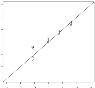
Thus, from theLR-test as well as from the graphical model check it is obvious that the data fit a simple Rasch model. Thus, the first condition for a LLTM fit is fulfilled. The subsequent graphical model test in Figure 3 shows that especially for the LLTM restrictions hold for all items. This plot can be produced with the following code:
R> x <- resrm$betapar
R> y <- scale(reslltm$betapar, scale = FALSE)
R> plot(x, y, main = "Graphical LLTM Model Test", xlab = "Beta RM", + ylab = "Beta LLTM", xlim = c(-3, 3), ylim = c(-3, 3), type = "p") R> text(x, y + 0.2, label = colnames(resrm$X))
R> abline(0, 1)
4.2. An ordinary RSM example
Again, we provide an artificial data set withn = 20 persons and k= 6 items; each of them withm+ 1 = 4 categories:
R> data("rsmdat") R> head(rsmdat)
● ● ● ● ● −3 −2 −1 0 1 2 3 −3 −2 −1 0 1 2 3
Graphical Model Check
Beta Group 1 Beta Group 2 I1 I2 I3 I4 I5
Figure 2: RM graphical model check
● ● ● ● ● −3 −2 −1 0 1 2 3 −3 −2 −1 0 1 2 3
Graphical LLTM Model Test
Beta RM Beta LLTM I1 I2 I3 I4 I5
[,1] [,2] [,3] [,4] [,5] [,6] [1,] 3 2 0 1 0 1 [2,] 1 1 1 1 0 3 [3,] 2 0 0 0 0 2 [4,] 0 2 0 0 1 0 [5,] 1 0 2 1 3 0 [6,] 1 2 2 1 0 0
The design matrixW is generated automatically which leads to
R> resrsm <- RSM(rsmdat) R> model.matrix(resrsm) [,1] [,2] [,3] [,4] [,5] [,6] [,7] [1,] 1 0 0 0 0 1 0 [2,] 2 0 0 0 0 0 1 [3,] 3 0 0 0 0 -1 -1 [4,] 0 1 0 0 0 1 0 [5,] 0 2 0 0 0 0 1 [6,] 0 3 0 0 0 -1 -1 [7,] 0 0 1 0 0 1 0 [8,] 0 0 2 0 0 0 1 [9,] 0 0 3 0 0 -1 -1 [10,] 0 0 0 1 0 1 0 [11,] 0 0 0 2 0 0 1 [12,] 0 0 0 3 0 -1 -1 [13,] 0 0 0 0 1 1 0 [14,] 0 0 0 0 2 0 1 [15,] 0 0 0 0 3 -1 -1 [16,] -1 -1 -1 -1 -1 1 0 [17,] -2 -2 -2 -2 -2 0 1 [18,] -3 -3 -3 -3 -3 -1 -1
The design matrixW consists ofk−1 = 5 item contrasts and (m+ 1)−2 = 2 item-category parameters. Thus, the vectorηbof the basic parameters estimated in the CML-routine consists
of 6 elements. The vectorβbrepresenting all estimable item×category parameters is the linear
combinationβb =Wηband has a total length of 18.
The summary method provides the log-likelihood value with corrsponding information criteria as well as theβ-estimates. TheLR-test, as described in Section3.2, is carried out using the
LRteststatement.
R> summary(resrsm)
Results of RSM fit:
Number of iterations: 16 Number of parameters: 7 AIC: 229.1236
BIC: 236.0938 cAIC: 243.0938
Item Parameters (beta): Parameter Estimate 1 beta I1.1 0.01903 2 beta I1.2 0.20546 3 beta I1.3 -0.08081 4 beta I2.1 -0.31007 5 beta I2.2 -0.45274 6 beta I2.3 -1.0681 7 beta I3.1 -0.26078 8 beta I3.2 -0.35416 9 beta I3.3 -0.92024 10 beta I4.1 -0.07223 11 beta I4.2 0.02295 12 beta I4.3 -0.35457 13 beta I5.1 0.15522 14 beta I5.2 0.47783 15 beta I5.3 0.32775 16 beta I6.1 0.43933 17 beta I6.2 1.04606 18 beta I6.3 1.18009
R> lrres <- LRtest(resrm, splitcr = "mean") R> lrres
Andersen LR-test: LR-value: 1.304053 df: 4
p-value: 0.8606874
The p-value of theLR-statistic suggests a satisfactory model fit.
4.3. An LPCM for repeated subgroups measures
The most complex example refers to an LPCM with two measurement points. In addition, the hypothesis is of interest whether the treatment has an effect. The corresponding contrast is the last column in W below.
First, the data matrix X is specified. We assume an artificial test consisting ofk = 3 items which was presented twice to the subjects. The first 3 columns inXcorrespond to the first test occasion, whereas the last 3 to the second occasion. Generally, the firstkcolumns correspond
to the first test occasion, the nextk columns for the second, etc. In total, there are n = 20 subjects. Among these, the first 10 persons belong to the first group (e.g., control), and the next 10 persons to the second group (e.g., treatment). This is specified by a group vector:
R> data("lpcmdat")
R> grouplpcm <- rep(1:2, each = 10)
Again, W is generated automatically. In general, for such designs the generation of W
consists first of the item contrasts, followed by the time contrasts and finally by the group main effects except for the first measurement point (due to identifiability issues, as already described).
R> reslpcm <- LPCM(lpcmdat, mpoints = 2, groupvec = grouplpcm, sum0 = FALSE) R> model.matrix(reslpcm) [,1] [,2] [,3] [,4] [,5] [,6] [,7] [,8] [,9] [,10] [1,] 0 0 0 0 0 0 0 0 0 0 [2,] 1 0 0 0 0 0 0 0 0 0 [3,] 0 1 0 0 0 0 0 0 0 0 [4,] 0 0 1 0 0 0 0 0 0 0 [5,] 0 0 0 1 0 0 0 0 0 0 [6,] 0 0 0 0 1 0 0 0 0 0 [7,] 0 0 0 0 0 1 0 0 0 0 [8,] 0 0 0 0 0 0 1 0 0 0 [9,] 0 0 0 0 0 0 0 1 0 0 [10,] 0 0 0 0 0 0 0 0 0 0 [11,] 1 0 0 0 0 0 0 0 0 0 [12,] 0 1 0 0 0 0 0 0 0 0 [13,] 0 0 1 0 0 0 0 0 0 0 [14,] 0 0 0 1 0 0 0 0 0 0 [15,] 0 0 0 0 1 0 0 0 0 0 [16,] 0 0 0 0 0 1 0 0 0 0 [17,] 0 0 0 0 0 0 1 0 0 0 [18,] 0 0 0 0 0 0 0 1 0 0 [19,] 0 0 0 0 0 0 0 0 1 0 [20,] 1 0 0 0 0 0 0 0 2 0 [21,] 0 1 0 0 0 0 0 0 3 0 [22,] 0 0 1 0 0 0 0 0 1 0 [23,] 0 0 0 1 0 0 0 0 2 0 [24,] 0 0 0 0 1 0 0 0 3 0 [25,] 0 0 0 0 0 1 0 0 1 0 [26,] 0 0 0 0 0 0 1 0 2 0 [27,] 0 0 0 0 0 0 0 1 3 0 [28,] 0 0 0 0 0 0 0 0 1 1 [29,] 1 0 0 0 0 0 0 0 2 2 [30,] 0 1 0 0 0 0 0 0 3 3 [31,] 0 0 1 0 0 0 0 0 1 1
[32,] 0 0 0 1 0 0 0 0 2 2
[33,] 0 0 0 0 1 0 0 0 3 3
[34,] 0 0 0 0 0 1 0 0 1 1
[35,] 0 0 0 0 0 0 1 0 2 2
[36,] 0 0 0 0 0 0 0 1 3 3
The parameter estimates are the following:
Basic Parameters eta:
eta 1 eta 2 eta 3 eta 4 eta 5 eta 6
Estimate -0.4615899 -1.609589 -0.5713665 -0.8388421 -1.739492 -0.7232787 Std.Err 0.7346631 1.194343 0.6232679 0.9854761 1.438194 0.6534217
eta 7 eta 8 eta 9 eta 10
Estimate -0.7096128 -1.209864 -0.2014868 1.0940434 Std.Err 0.9862337 1.414822 0.2608240 0.3870403
Testing whether the η-parameters equal 0 is mostly not of relevance for those parameters referring to the items (in this exampleη1, ..., η8). But for the remaining contrasts,H0 :η9 = 0
(implying no general time effect) can not be rejected (p=.44), whereas hypothesisH0 :η10=
0 has to be rejected (p=.004) when applying az-test. This suggests that there is a significant treatment effect over the measurement points. If a user wants to perform additional tests such as a Wald test for the equivalence of twoη-parameters, the vcov method can be applied to get the variance-covariance matrix.
5. Discussion and outlook
In this paper some theoretical as well as practical considerations have been presented with respect to the application of theeRmpackage. All the presented models fulfill the basic Rasch properties and are estimable by using a unified CML approach. If missing values occur in
X they are coded as NA. For each subgroup due to the NA structure, the likelihood value is computed separately. The corresponding theoretical treatment can be found inFischer and Ponocny(1994).
A further implication refers to the estimation of the person parameters. Due to the mentioned separability of item and person parameters, they do not need to be estimated simultaneously with the item parameters. If no assumptions are posed on the latent distribution f(θ),
Andersen(1995) gives a general formulation of the ML estimate ofθwithrv =r andθv =θ:
r− k X i=1 mi X h=1 hexp(hθ+βbih) Pmi l=0exp(hθv+βbil) = 0 (14)
The CML estimates forηbare inserted into Equation 7 in order to obtain the β-parameters.
Thus, considering all βbih to be known, Equation14 can be solved with respect to θ by using
the Newton-Raphson method. This is carried out by using the function person.parameter
In addition residuals and consequently, itemfit and personfit statistics are implemented as well as plot routines to visualize both empirical and estimated ICCs.
The last remark concerns additional models whose implementation in theeRmpackage could be an issue of future work. Thelinear logistic model with relaxed assumptions (Fischer 1977), abbreviated to LLRA, dispenses the uni-dimensionality requirement of the RM. The repa-rameterization θv −βi =: θvi leads to a generalization of the RM with θvi as independent
trait parameters. Applications of this model for the analysis of change as well as the formal equivalence of the LLRA and the LLTM (by introducing the concept if virtual persons) are described inFischer (1995b). Due to this equivalence, CML estimation can be applied. This estimation approach, in combination with the EM-algorithm, can also be used to estimate
mixed Rasch models (MIRA). The basic idea behind such models is that the extended Rasch model holds within subpopulations of individuals, but with different parameter values for each subgroup. Corresponding elaborations are given inRost and von Davier(1995).
To conclude, theeRmpackage is a tool to estimate extended Rasch models for unidimensional traits. The generalizations towards different numbers of item categories, linear extensions in terms of trend and group contrasts are important issues when examining item behavior and person performances in tests. This improves the feasibility of IRT models with respect to a wide variety of application areas.
References
Andersen EB (1972). “The Numerical Solution of a Set of Conditional Estimation Equations.”
Journal of the Royal Statistical Society, Series B,34, 42–54.
Andersen EB (1973). “A Goodness of Fit Test for the Rasch model.” Psychometrika, 38, 123–140.
Andersen EB (1983). “A General Latent Structure Model for Contingency Table Data.” In H Wainer, S Messik (eds.), “Principals of Modern Psychological Measurement,” pp. 117–138. Erlbaum, Hillsdale, NJ.
Andersen EB (1995). “Polytomous Rasch Models and their Estimation.” In G Fischer, I Mole-naar (eds.), “Rasch models: Foundations, Recent Developments, and Applications,” pp. 271–292. Springer, New York.
Anderson C, Li Z, Vermunt J (2007). “Estimation of Models in the Rasch Family for Poly-tomous Items and Multiple Latent Variables.”Journal of Statistical Software,20(6). URL
http://www.jstatsoft.org/v20/i06/.
Andrich D (1978). “A Rating Formulation for Ordered Response Categories.”Psychometrika, 43, 561–573.
Baker FB, Kim S (2004). Item Response Theory: Parameter Estimation Techniques. Dekker, New York, 2nd edition.
Borsboom D (2006). “The Attack of the Psychometricians.”Psychometrika,71, 425–440. de Leeuw J, Verhelst N (1986). “Maximum Likelihood Estimation in Generalized Rasch
Fischer GH (1973). “The Linear Logistic Test Model as an Instrument in Educational Re-search.”Acta Psychologica,37, 359–374.
Fischer GH (1974). Einf¨uhrung in die Theorie psychologischer Tests [Introduction to Mental Test Theory]. Huber, Bern.
Fischer GH (1977). “Linear Logistic Trait Models: Theory and Application.” In H Spada, WF Kempf (eds.), “Structural Models of Thinking and Learning,” pp. 203–225. Huber, Bern.
Fischer GH (1995a). “Derivations of the Rasch Model.” In G Fischer, I Molenaar (eds.), “Rasch Models: Foundations, Recent Developments, and Applications,” pp. 15–38. Springer, New York.
Fischer GH (1995b). “Linear Logistic Models for Change.” In G Fischer, I Molenaar (eds.), “Rasch Models: Foundations, Recent Developments, and Applications,” pp. 157– 180. Springer, New York.
Fischer GH, Parzer P (1991). “An Extension of the Rating Scale Model with an Application to the Measurement of Change.”Psychometrika,56, 637–651.
Fischer GH, Ponocny I (1994). “An Extension of the Partial Credit Model with an Application to the Measurement of Change.”Psychometrika,59, 177–192.
Fischer GH, Ponocny-Seliger E (1998). Structural Rasch Modeling: Handbook of the Usage of LPCM-WIN 1.0. ProGAMMA, Groningen.
Fisher Jr WP (1992). “Objectivity in Measurement: A Philosophical History of Rasch’s Separability Theorem.” In M Wilson (ed.), “Objective Measurement: Theory into Practice, Volume 1,” pp. 29–60. Ablex, Norwood, NJ.
Glas CAW (1992). “A Rasch Model with a Multivariate Distribution of Ability.” In M Wilson (ed.), “Objective Measurement: Theory into Practice, Volume 1,” pp. 236–258. Ablex, Norwood, NJ.
Glas CAW, Verhelst N (1989). “Extensions of the Partial Credit Model.”Psychometrika,54, 635–659.
Glas CAW, Verhelst N (1995). “Tests of Fit for Polytomous Rasch Models.” In G Fischer, I Molenaar (eds.), “Rasch Models: Foundations, Recent Developments, and Applications,” pp. 325–352. Springer, New York.
Hoijtink H (1995). “Linear and Repeated Measures Models for the Person Parameter.” In G Fischer, I Molenaar (eds.), “Rasch Models: Foundations, Recent Developments, and Applications,” pp. 203–214. Springer, New York.
Kubinger KD (2005). “Psychological Test Calibration Using the Rasch model - Some Critical Suggestions on Traditional Approaches.” International Journal of Testing,5, 377–394. Liou M (1994). “More on the Computation of Higher-Order Derivatives of the Elementary
Masters GN (1982). “A Rasch Model for Partial Credit Scoring.”Psychometrika,47, 149–174.
Mislevy RJ (1985). “Estimation of Latent Group Effects.”Journal of the American Statistical Association,80, 993–997.
Pfanzagl J (1994). “On Item Parameter Estimation in Certain Latent Trait Models.” In G Fischer, D Laming (eds.), “Contributions to Mathematical Psychology, Psychometrics, and Methodology,” pp. 249–263. Springer, New York.
R Development Core Team (2006). R: A Language and Environment for Statistical Comput-ing. R Foundation for Statistical Computing, Vienna, Austria. ISBN 3-900051-07-0, URL
http://www.R-project.org.
Rasch G (1960). Probabilistic Models for Some Intelligence and Attainment Tests. Danish Institute for Educational Research, Copenhagen.
Rasch G (1961). “On General Laws and the Meaning of Measurement in Psychology.” In “Proceedings of the IV. Berkeley Symposium on Mathematical Statistics and Probability,
Vol. IV,” pp. 321–333. University of California Press, Berkeley.
Rasch G (1977). “On Specific Objectivity: An Attempt at Formalising the Request for Generality and Validity of Scientific Statements.” Danish Yearbook of Philosophy, 14, 58–94.
Rizopoulos D (2006). “ltm: An R Package for Latent Variable Modeling and Item Re-sponse Theory Analyses.” Journal of Statistical Software, 17(5), 1–25. URL http: //www.jstatsoft.org/v17/i05/.
Rost J (1999). “Was ist aus dem Rasch-Modell geworden? [What Happened with the Rasch Model?].” Psychologische Rundschau,50, 140–156.
Rost J, von Davier M (1995). “Polytomous Mixed Rasch Models.” In G Fischer, I Molenaar (eds.), “Rasch Models: Foundations, Recent Developements, and Applications,” pp. 371– 382. Springer, New York.
Scheiblechner H (1972). “Das Lernen und L¨osen komplexer Denkaufgaben. [The Learning and Solving of Complex Reasoning Items.].” Zeitschrift f¨ur Experimentelle und Angewandte Psychologie,3, 456–506.
Affiliation:
Patrick Mair
Department f¨ur Statistik und Mathematik Wirtschaftsuniversit¨at Wien
A-1090 Wien, Austria
E-mail: [email protected]
URL:http://statmath.wu-wien.ac.at/~mair/
Journal of Statistical Software
http://www.jstatsoft.org/published by the American Statistical Association http://www.amstat.org/
Volume 20, Issue 9 Submitted: 2006-10-01