Traffic fundamentals for A22 Brenner freeway by microsimulation models.

(1)

Department of Civil, Environmental, Aerospace, Materials Engineering

PhD IN CIVIL AND ENVIRONMENTAL ENGINEERING Transportation Infrastructures Engineering and Geomatics

CICLE XXVI – S.S.D. ICAR/04 PhD THESIS

Traffic fundamentals for A22 Brenner freeway by microsimulation models.

PhD Candidate Coordinator

Ing. Sandro Chiappone Prof. Eng. Orazio Giuffrè

Supervisors

Prof. Eng. Anna Granà Prof. Eng. Raffaele Mauro

(2)

Department of Civil, Environmental, Aerospace, Materials Engineering

PhD IN CIVIL AND ENVIRONMENTAL ENGINEERING Transportation Infrastructures Engineering and Geomatics

CICLE XXVI – S.S.D. ICAR/04 PhD THESIS

Traffic fundamentals for A22 Brenner freeway by microsimulation models.

PhD Candidate Coordinator

Ing. Sandro Chiappone Prof. Eng. Orazio Giuffrè

Supervisors

Prof. Eng. Anna Granà Prof. Eng. Raffaele Mauro

(3)

iii

ACKNOWLEDGEMENT

I am very much thankful to my tutors Professor Anna Granà and Professor Raffaele Mauro for their interest and encouragement during my PhD period.

I also express my gratitude to Professor Ana Bastos Silva for her humane and academic support during my foreign stay in University of Coimbra.

I express deep and sincere gratitude to Professor Orazio Giuffrè whose guidance, encouragement and fundamental suggestion have contributed to the evolution of my ideas on the project.

I am also thankful to Dr. Eng. Daniela Condino for her important suggestions and advices.

I would like to express my gratitude to Fabiola for her constant support during the difficult moments of my PhD.

I am extremely thankful to my family for her constant encouragement throughout my research period.

(4)

I. FOREWORD

I.1 GENERALITIES

Road traffic microsimulation models are one of the latest generation of available traffic models and became very popular for the development and evaluation of a broad range of road traffic management and control systems. They model the movements of individual vehicles, traveling around road networks by using car following, lane changing and gap acceptance rules; hence, traffic microsimulation models try to replicate the behavior of individual drivers. However, the "realism" sought by the representation of individual drivers introduces a level of complexity into the modeling process which must be taken into account from the stage of model calibration. Traffic microsimulation models typically include a very large number of parameters, representing various characteristics of travelers, vehicles and road system, that must be calibrated before the model is applied as a prediction tool of traffic performances (Hollander and Liu, 2008).

Microsimulation models are the ones closer to reality in the reproduction of the traffic system opening a wide range of traffic scenarios in which

(8)

precise descriptions of traffic control and traffic management schemes can be explicitly included.

Microsimulation traffic models can produce visual outputs by which lay and technical people can discuss the respective merits of traffic and transport proposals. The models can represent road and transport networks and their operation and the behaviour of vehicles and travelers in more detail, and broaden the range of applications. The visual representation of problems and solutions in a format understandable to lay people, project managers and modellers is a useful way to gain more widespread acceptance of complex strategies.

I.2 THE AIMS OF THIS PHD THESIS

In this work of PhD Thesis a methodology to find fundamentals diagrams by microsimulations will be presented.

As it is know from scientific literature, the fundamental diagram relates two of the three variables: average speed (v), flow (q) and density (k) to each other. If two of these variables are known, the third can be derived using the relation q = kv. Therefore, if only one variable is known, and the fundamental diagram is known, the traffic state can be determined. The fundamental relationship is largely used in road infrastructure engineering, e.g. in the level-of-service evaluation of basic freeway or multilane segments.

(9)

3 The present work of PhD thesis starts by introducing the fundamental diagram using Edie’s definitions and the use of speed- density diagrams. Another objective will be to analyzed a method that include an automated technique based on genetic algorithm (GA) for automating the process of calibration of the parameters in order to reproduce the fundamentals diagrams of the A22 Brenner freeway.

A further important objective will be to evaluate the impact of heavy vehicle on the quality of flow of the A22 Brenner freeway by calculating the Passenger Car Equivalents Factor (PCEs) between heavy vehicles and cars based on the results obtained in microsimulation. The calculation of PCE (Passenger Car Equivalents) will be done in general terms in order to compare the results with those published in the Highway Capacity Manual (HCM, 2010) resulting from experimental studies.

I.3 ORGANIZATION OF THE THESIS

The present PhD thesis consists of four chapters that illustrate the work of study and research that has been developed during the PhD course. The chapter one is a background that describes the traffic modeling techniques available in the scientific literature with particular attention to microscopic simulation models. In particular it will be explained the benefit and the advantage of using Traffic Microsimulation Models for freeways.

(10)

In the second chapter a statistical approach based on observed and simulated speed-density relationships will be applied in the calibration process to measure the closeness between empirical data and simulation outputs. The comparison established between the lnS-D2_linear

regressions (where S is for Speed and D is for density) for all simulated values and the corresponding linear regressions for the empirical data will allow to evaluate the quality of the calibration of the traffic microsimulation model. Furthermore, a statistical approach including hypothesis testing using t-test and confidence intervals will be used.

In the third chapter, the most important models for the analytical calculation of PCEs (Passenger Car Equivalents) will be presented and the Aimsun software performance will be tested. After that, the results of microsimulations in Aimsun will be evaluated in order to obtain the relevant parameters for the estimation of the PCEs and their comparison with those proposed by HCM.

Finally, the last chapter will show the first results obtained by applying a genetic algorithm in the microsimulation traffic model calibration process. The calibration will be formulated as an optimization problem in which the objective function was defined to minimize the differences of the simulated measurements from those observed in the speed-density diagram.

(11)

5

I. TRAFFIC SIMULATION MODELS

Simulation is a process based on building a computer model that suitably represents a real or proposed system which enables the extraction of valid inferences on the behavior of the modeled system, from the outcomes of the computer experiments conducted on its model. Simulation has become, in recent years, one of the most used and powerful tools for systems analysis and design, by its proven ability to answer "what if" questions helping the system designer to find solutions for building new systems, or assess the impact of proposed changes on an already existing system. A simulation model is always a simplified representation of a system that addresses specifically those aspects of the studied system relevant for the purposes of the analysis from the point of view of the system analyst. A simulation model is therefore specific, both for the problem and for whoever tries to use the model for finding solutions to

(12)

the problem. A simulation study has usually the objective of helping to achieve a better understanding on how a system behaves, evaluating the impact of changes in the system, or in values of the parameters governing the system, or of decisions on the policies controlling the system.

Mathematical modelling of traffic flow behaviour is a prerequisite for a number of important tasks including transportation planning, traffic surveillance and monitoring, incident detection, systematic control strategy design, simulation, forecasting and, last but not least, more recently in evaluating energy consumed by transportation systems, environmental impacts due to transportation systems, and in assessing vehicle guidance systems (Barce1ò et al., 1995a, 1995b).

Furthermore, traffic modelling plays an important part in the assessment of a range of traffic schemes, whether these are new road schemes, junction improvements, changes to traffic signal timings or the impact of transport telematics. There is a wide range of alternative modelling approaches now available based on macro- or micro-simulation methods. Micro-simulation models differ significantly from traditional transport models in terms of their methodology and supporting algorithms.

The management of a road network often requires the forecasting of the impacts of implementing various traffic management measures. These measures include, for example, signal coordination, high occupancy vehicle (HOV) lanes, one-way systems, different types of intersection control (priority sign, signal or roundabout), signal priority, driver

(13)

7 information systems and incident management. Apart from road vehicles, trams, light rails, pedestrians and cyclists can also be simulated

Traffic modelling techniques can be broadly classified into the following four types:

a) Analytical modelling – this technique relates directly to traffic flow theory and is often a set of equations governing driver behaviour such as gap acceptance, lane changing, car– following, or platoon dispersion. The combination of analytical models can constitute a more complex analytical model for traffic analysis. Individual sets of analytical equations can also act as sub-models in other modelling techniques. Analytical modelling is sometimes also known as microscopic modelling.

b) Microscopic Simulation - the movement of a vehicle in a microscopic simulation is traced through a road network over time at a small time increment of a fraction of a second. A detailed simulation of vehicle-road interaction under the influence of a control measure is therefore possible. This technique is useful for a wide range of applications but requires more computational resources. Random number generators are involved and the calibration of these models requires more effort, and it is difficult to optimise model parameters.

(14)

c) Macroscopic Simulation - vehicles in a macroscopic simulation are no longer simulated individually. Vehicle movements are often simulated as packets or bunches in a network with a time step of one or several seconds. An analytical model such as the platoon dispersion model is used to govern the movement of a vehicle platoon along a road link. A macroscopic simulation is deterministic by nature and is useful for network design and optimization.

d) Mesoscopic simulation – this technique combines a detailed microscopic simulation of some key components of a model (e.g. intersection operations) with analytical models (e.g. speedflow relationships for traffic assignment). This technique is sometimes known as mesoscopic simulation and provides more detail to what is normally an assignment only model. It is also possible to interface a microsimulation model with a real-time signal control system such as SCATS - an area of active research and development at RTA NSW (Millar et al. 2006).

In recent years, Intelligent Transport System (ITS) measures such as adaptive signal control algorithms, incident management strategies, active bus/tram priority and driver information systems have been introduced to freeways and arterial roads. These are complex traffic processes and traffic flow theories are often unable to accurately predict the impacts in terms of delay, queue length, travel times, fuel

(15)

9 consumption and pollutant emissions. Computer models equipped with advanced graphical facilities have been developed in recent years to meet the needs of a road manager.

Computer software has long been developed to simulate traffic management processes amongst road authorities in Australia (e.g. Cotterill et al. 1984; Tudge 1988). Past research also includes the development of car-following and lane changing algorithms for microsimulation (Gipps 1981 and 1986), the review of eight small area traffic management models, and the comparison of macroscopic and microscopic simulations (Luk and Stewart 1984; Ting et al. 2004). More recent research includes the assessment and further development of car-following and lane changing algorithms (Hidas 2005; Panwai and Dia 2004). A key finding is that microscopic simulation models require careful calibration to produce meaningful results, especially in the lane changing behaviour in congested conditions.

I.1 BENEFITS OF MICROSCOPIC TRAFFIC SIMULATION MODELS

Micro-simulation models have the ability to model each individual vehicle within a network. In theory, such models should provide a better representation of actual driver behavior and network performance, particularly when networks are approaching capacity and vehicle interactions become far more important in determining the outturn

(16)

operational performance. They are the only modelling tools available with the capacity to examine certain complex traffic problems (e.g. junctions, shockwaves, effects of incidents, interaction with pedestrian traffic etc.). In addition, there is the appeal to users of the powerful graphics offered by most micro-simulation packages. Whilst this can provide decision makers and consultee’s graphical representation of the performance of a scheme it should never be the only reason for using micro-simulation.

Microsimulation can potentially offer benefits over traditional traffic analysis techniques in three areas: clarity, accuracy and flexibility as follows:

 Clarity - a comprehensive real-time visual display and graphical user interface illustrate traffic operations in a readily understandable manner. The animated outputs of microsimulation modelling are easy to understand and simplify checking that the network is operating as expected, and whether driver behaviour is being modelled sensibly. With microsimulation, what you see is what you get. If a microsimulation model does not look right, then it probably is not right, and vice versa;

 Accuracy - by modelling individual vehicles through congested networks, the potential exists for more accurate modelling of traffic operations at complex and simple intersections or merges. Individual drivers of vehicles make their own decision on speed,

(17)

11 lane changing and route choice, which could better represent the real world than other modelling techniques. For examples, analytical and macrosimulation models often use fixed value of saturation flows and all vehicles are assumed to behave in the same manner. In contrast, microsimulation models represent individual vehicles and detailed networks. A parameter such as the saturation flow can actually be an output of the model;

 Flexibility - a greater range of problems and solutions can be assessed than with conventional methods, e.g. vehicle-activated signals, demand dependent pedestrian facilities, queue management, public transport priorities, incidents, toll booths, road works, signalised roundabouts, shock waves, incidents or flow breakdown, or slip road merges.

Dowling et al. (2002) lists the following as study conditions where micro simulation models are desirable:

 Conditions that violate one or more basic assumptions of independence required by HCM models

o Queues spill back from one intersection to another o Queues overflow turn pockets

o Queues from city streets back up onto freeways o Queues from ramp meters back up onto city streets

(18)

 Conditions not covered well by available HCM models o Queue spill-back

o Multi-lane with traffic signals or stop signs o Truck climbing lanes

o Short through lane adds or drops at a signal

o Boundary points between different signal systems operating at different cycle lengths

o Signal pre-emption (e.g., railroad crossings and fire stations)

o HOV lane entry options or design options for starting or ending an HOV lane

o Two lanes turning left (however, currently no commercially available micro simulation software can model this)

o Roundabouts

o Tight diamond interchanges

o Incident management options (Because HCM and macroscopic models assume a steady-state condition within each analysis period, they are not well suited to accurately track the build-up and dissipation of congestion related to random transitory conditions caused by incidents.)

(19)

13 In this regard, Transport of London (2003) lists the following issues as being suitable for microscopic simulation models:

 Complex traffic operation schemes (e.g., bus priority, advanced signal control, incident management, different modes of toll collection);

 Significant conflicts among different road users (e.g., pedestrians, cyclists, buses);

 Major traffic movement restrictions (e.g., lane closures, one-way system, toll plazas);

 Politically sensitive projects that could benefit from visualization;  Planning and design of high-value projects with potential large

savings if detailed microscopic simulation models are prepared;  Emulation of the operation of a dynamic signal control system,

with a simulated network driven directly by the control system and with significant saving in signal timing preparation and optimization;

 Town center studies;

 Tram and light rail operations.

However, there are some limitations to consider in microsimulation models. In this respect, it is always beneficial to restate Dr. May’s observations regarding the use of micro simulation (May 1990):

(20)

 There may be easier ways to solve the problem; consider all possible alternatives;

 Micro simulation can be time-consuming and expensive; do not underestimate time and cost;

 Micro simulation packages require considerable input characteristics and data, which may be difficult or impossible to obtain;

 Micro simulation applications or models require calibration, validation and verification, or auditing, which if overlooked could make the model useless;

 Development of simulation models requires knowledge in a variety of disciplines, including traffic flow theory, computer programming and operation, probability, decision-making, and statistical analysis;

 Micro simulation is difficult unless the model developer fully understands the software platform;

 The micro simulation package may be difficult for non-developers to use because of lack of documentation or unique computer facilities;

 Some users may apply micro simulation packages and treat them as black boxes and really do not understand what they represent;  Some users may apply simulation models and not know or

(21)

15 The scale of application of microsimulation models depends on the size of the computer memory and on the computer power available. Models that have not been built to run simulations on large networks but rather to achieve highly specific objectives have a small scale of application, typically less than one hundred vehicles. The scale of application ranges tipically varies from about 20 km, 50 nodes, and one thousand vehicles, to a large application of 200 nodes and many thousands of vehicles. With the increasing application of micro-simulation models, there is a need for advice on their development and application, particularly in the context of the motorway and trunk road network. Key issues to be addressed include how well and under what conditions or constraints micro-simulation works and offer the greatest benefits. The calibration, validation and subsequent performance of any model are fundamental and, sometimes, contentious issues. The variables that are taken into account in micro-simulation models have lead to questions as to the validity of the results obtained and the degree to which confidence can be placed on the modelling.

I.2 IMPROVING DECISION-MAKING BY USING MICROSIMULATION MODELS

In reality, there are a large number of situations where micro simulation led to better investment decisions and more effective designs. There are likely to be situations where simulation models provided faulty

(22)

predictions, but these projects were not included in the web survey. It is probably safe to assume, however, that a properly calibrated and validated microscopic simulation model will more often than not lead to more effective designs and investment decisions because it can more closely replicate what is likely to occur in the real world.

Suggesting that a design is better or more effective is either a subjective opinion or it requires some basis of comparison. In most of the cases reported in the web survey, the assessment was based on a comparison to prior studies using traditional models or HCM calculations. For example, an intersection designed as an all-way stop using traditional traffic engineering calculations did not perform as expected in the real world. A microscopic simulation was then used to confirm the observed behavior and develop a more effective design for the intersection. The evaluation led to the decision that traffic would be better served if the intersection was configured as a round-about.

Micro simulation modeling has also proved useful in situations that are outside the bounds of traditional techniques. These can include odd or complex intersection configurations or heavily congested arterials. For example, a heavily congested arterial with two cross streets 120 feet apart could not be designed using traditional stop sign or signalization calculations. A round-about option was modeled using micro simulation with the software providing guidance on the appropriate diameter for the round-about, whether it required a single or dual lane circle, and how

(23)

17 queuing on minor approaches would be eliminated. In addition, the model was able to show that driveways for existing businesses around the proposed round-about would be too close to the traffic circulating. The tool provided the data needed to relocate the driveways a safe distance from the round-about. In fact, there are a large number of studies and real cases that show the benefits of micro simulation for improved decision-making.

I.3 TRAFFIC SIMULATION WITH AIMSUN

Aimsun by Ferrer and Barcelò (1993) is a software tool able to reproduce the real traffic conditions on an urban network which may include both expressways and arterial routes. It is based on a microscopic simulation approach. The behavior of each single vehicle which is present in the network is continuously modeled throughout the simulation time period, according to several driver behavior models (car following, lane changing, gap acceptance). Having outgrown the stated aim of the original Aimsun acronym ‘advanced interactive microscopic simulator for urban and non-urban networks’ (Ferrer and Barceló, 1993; Barceló et al., 1994, 1998a), the software now includes macroscopic, mesoscopic and microscopic models and is simply known as ‘Aimsun’ (Aimsun, 2008). Expanding in response to practitioners’ requirements, Aimsun has come to encompass a collection of dynamic modelling tools. Specifically,

(24)

these include mesoscopic and microscopic simulators and dynamic traffic assignment models based on either user equilibrium or stochastic route choice. From a practitioner’s standpoint, macroscopic modelling plays an increasingly important role in the area of demand data preparation. The primary areas of application for Aimsun are offline traffic engineering and, more recently, online (real-time) traffic management decision support. In either case, the use of Aimsun, or Aimsun Online, aims to provide solutions to short and medium term planning and operational problems for which the dynamic and disaggregate models described in this chapter are extremely well suited. Strategic planning is an adjacent realm for which more aggregate and/or static models continue to be very suitable. There are important interfaces between those two realms at the level of methodology (effect on demand of lasting changes to the effective capacity) and technology (importing from and exporting data to strategic planning software) and these will be commented upon further in the following sections.

I.3.1 MODEL BUILDING PRINCIPLES IN AIMSUN

Building a transport simulation model with Aimsun is an iterative procedure that comprises three steps:

 Model building, that is, the procedure of gathering and processing the inputs to create the model;

(25)

19  Verification, calibration and validation, that is the process

of confirming that implementation of the model logic is correct; setting appropriate values for the parameters and comparing the outputs of the model to correspond with realworld measurements in order to test its validity;

 Output analysis, explores the outputs of model in line with the overall objectives of the modelling study.

In the next section, some key elements of the Aimsun Traffic Microsimulation model will be focused upon.

I.3.2 MODEL VERIFICATION, CALIBRATION AND

VALIDATION

Before starting to modify the model parameters in order to calibrate the model, the user must be sure that there are no specification errors that affect the model logic and therefore simulation results. Verification consists in assuring that the model has been correctly edited in Aimsun, checking network geometry, control plans, management strategies and traffic demand, and verifying that the model description corresponds to the objectives of the study. Aimsun provides a tool that can automatically detect errors in supply definition, such as a section where not all the lanes at the beginning or at the end are connected or an OD pair with trips but

(26)

no feasible path. Verification of traffic demand is carried out through a manual comparison with traffic counts wherever possible; for example the total trips generated and attracted by a zone must be compared with the counts of the sections to which the corresponding centroid is connected. An important check is to verify that the model is suitable for the objectives of the study; the model must include all the area that might be influenced by future changes being modelled; the boundaries must be free of congestion; if rerouting strategies are simulated, then alternative paths must be possible in the network being modelled; OD matrices should be time sliced so as to reproduce traffic demand dynamics correctly and the study time frame must extend beyond (earlier than) the peak hour to avoid starting the simulation in an oversaturated condition. Calibration is an iterative process that consists of changing model parameters and comparing model outputs with a set of real data until a predefined level of agreement between the two data sets is achieved. Which output needs to be generated depends on the type of model (macro, meso or micro), the objective of the study and the type of network. The most significant measures for a highway model are the relationship between speed/flow/density, lane utilization and congestion propagation.

(27)

21 I.3.3 AIMSUN CORE MODEL: CAR FOLLOWING AND LANE

CHANGING

The core models in Aimsun deal with individual vehicles, each vehicle/driver having behavioral attributes assigned to them when they enter the system; those attributes remain constant during the whole trip. The difference between the core models at the mesoscopic and microscopic levels relates to the level of abstraction and to the process employed to update each vehicle’s status. Accordingly, in what follows, two sets of fundamental core models: microscopic behavioral models and mesoscopic behavioral models are described separately.

In the Aimsun micro-simulator, during a vehicle’s journey along a route in the network, its position is updated according to two driver behavior models termed ‘car following’ and ‘lane changing’.

The premise behind the models is that drivers tend to travel at their desired speed in each road section but the environment (i.e. preceding vehicle, adjacent vehicles, traffic signals, signs, blockages, etc.) conditions their behavior. Simulation time is split into small time intervals called simulation cycles or simulation steps. At each simulation step, the position and speed of every vehicle in the system is updated according to the algorithm of the lane changing and car following model. Once all vehicles have been updated for the current simulation step, vehicles scheduled to arrive during this cycle are introduced into the system and the next vehicle arrival times are generated.

(28)

I.3.4 MICROSCOPIC CAR FOLLOWING MODEL

The car-following model implemented in Aimsun is based on the model proposed by Gipps (Gipps, 1986). It can actually be considered an evolution of this empirical model, in which the model parameters are not global but determined by the influence of local parameters depending on the type of driver (speed limit acceptance of the vehicle), the road characteristics (speed limit on the section, speed limits on turnings, etc.), the influence of vehicles on adjacent lanes, etc. The model consists of two components: acceleration and deceleration. The first represents the intention of a vehicle to achieve a certain desired speed, while the second reproduces the limitations imposed by the preceding vehicle when trying to drive at the desired speed.

This model states that the maximum speed to which a vehicle (n) can accelerate during a time period (t, t+T) is given as:

) n ( * V ) t , n ( V 025 , 0 ) n ( * V ) t , n ( V 1 T ) n ( a 5 , 2 ) t , n ( V ) T t , n ( V_a _              where:

 V(n,t) is the speed of the vehicle n at time t;

 a(n) is the maximum acceleration for the vehicle n;

 T is the reaction time;

(29)

23 On the other hand, the maximum speed that the same vehicle (n) can reach during the same time interval (t, t+ T), according to its own characteristics and the limitations imposed by the presence of the lead vehicle (n−1), is:





} 1) (n d' t) 1, (n V T t) V(n, t) x(n, 1) s(n t) 1, x(n d(n){2 T (n) d T d(n) T) t (n, V 2 2 2 b                 Where:

 d(n) is the maximum deceleration desired by vehicle n;

 x(n, t) is the position of the vehicle n at time t;

 x(n–1, t) is the position of the preceding vehicle (n−1) at time t;

 s(n–1, t) is the effective length of the vehicle (n−1);

 d(n–1) is an estimate of the vehicle (n−1) desired deceleration. The speed of the vehicle (n) during time interval (t, t+T) is the minimum of the two expressions above:



V (n,t T);V (n,t T)



min

T) t

V(n,   _a  _b 

Then, the position of the vehicle n inside the current lane is updated taking this speed into the movement equation:

(30)

T T) t V(n, t) x(n, T) t x(n,     

The car-following model is such that a leading vehicle, i.e. a vehicle driving freely without any vehicle affecting its behavior, would try to drive at its maximum desired speed. Three parameters are used to calculate the maximum desired speed of a vehicle while driving on a particular section or turning; of these, two are related to the vehicle and one to the section or turning. Specifically:

 Maximum desired speed of the vehicle i: vmax(i)  Speed acceptance of the vehicle i: θ(i)

 Speed limit of the section or turning s: Slimit(s)

The speed limit for a vehicle i on a section or a turning s, slimit(i, s), is

calculated as follows: ) ( S (i) ) (i, S_limit s   _limit s

Then, the maximum desired speed of the vehicle i on a section or a turning s, vmax(i, s), is calculated as follows:



S (i, );V (i)



min

) (i,

V_max s  _limit s _max

This maximum desired speed vmax(i, s) is the same as that referred to

above, in the Gipps’ car-following model, as V∗(n).

The car-following model proposed by Gipps is a one-dimensional model that considers only the vehicle and its leader. However, the implementation of the car following model in Aimsun also considers the

(31)

25 influence of adjacent lanes. When a vehicle is driving along a section, we consider the influence that a certain number of vehicles driving slower in the adjacent right-side lane – or left-side lane when driving on the left – may have on the vehicle. The model determines a new maximum desired speed of a vehicle in the section, which will be used in the car following model, considering the mean speed of vehicles driving downstream of the vehicle in the adjacent slower lane and allowing a maximum difference of speed.

I.3.5 LANE CHANGING MODEL

The lane-changing model can also be considered as a development of the Gipps lane-changing model (Gipps, 1986). Lane change is modelled as a decision process, analysing the necessity of the lane change (such as for turning manoeuvres determined by the route), the desirability of the lane change (to reach the desired speed when the leader vehicle is slower, for example), and the feasibility conditions for the lane change that are also local, depending on the location of the vehicle in the road network. The lane-changing model is a decision model that approximates the driver’s behaviour in the following manner: each time a vehicle has to be updated, we ask the following question: Is it necessary or desirable to change lanes? The answer to this question will depend on the distance to the next turning and the traffic conditions in the current lane. The traffic conditions are measured in terms of speed and queue lengths. When a driver is going slower than he wishes, he tries to overtake the preceding

(32)

vehicle. On the other hand, when he is travelling fast enough, he tends to go back into the slower lane. If we answer the previous question in the affirmative, to successfully change lanes, we must first answer two further questions:

 “Is there benefit to changing lane?” Check whether there will be any improvement in the traffic conditions for the driver as a result of lane changing. This improvement is measured in terms of speed and distance. If the speed in the future lane is fast enough compared to the current lane, or if the queue is short enough, then it is beneficial to change lanes;

 “Is it feasible to change lanes?” Verify that there is sufficient gap to make the lane change with complete safety. For this purpose, we calculate both the braking imposed by the future downstream vehicle to the changing vehicle and the braking imposed by the changing vehicle to the future upstream vehicle. If both braking ratios are acceptable, then the lane change is possible.

In order to achieve a more accurate representation of the driver’s behaviour in the lane-changing decision process, three different zones inside a section are considered, each one corresponding to a different lane-changing motivation. These zones are characterized by the distance up to the end of the section, i.e., the next point of turning (see Fig. 1.1).

(33)

27 conditions of the lanes involved. The necessity of a future turning movement is not yet taken into account. To measure the improvement that the driver will achieve by changing lanes, we consider several parameters: desired speed of driver, speed and distance of current preceding vehicle, speed and distance of future preceding vehicle in the destination lane;

 Zone 2: This is the intermediate zone. It is mainly the desired turning lane that affects the lane-changing decision. Vehicles not driving in valid lanes (i.e. lanes where the desired turning movement can be made) tend to get closer to the correct side of the road from which the turn is allowed. Vehicles looking for a gap may try to adapt to it but do not yet affect the behaviour of vehicles in the adjacent lanes.

 Zone 3: This is the shortest distance to the next turning point. Vehicles are forced to reach their desired turning lanes, reducing speed if necessary, and even come to a complete stop (gap forcing) in order to make the change possible. Within this zone, vehicles in the adjacent lane may also modify their behaviour (courtesy yielding) in order to provide a gap big enough for the vehicle to succeed in changing lanes.

(34)

Figure 1.1 Lane-changing zones

The lane changing of each vehicle i at section s could be summarized with the following elements:

 Lane Changing zone distance calculation;

 Target Lanes calculation;

 Vehicle behaviour considering the target lanes;

 Gap Acceptance model;

 Target Gap and Cooperation.

The “Lane changing zones” are defined by two parameters, at level of turning, Distance to Zone 1 and Distance to Zone 2. These parameters are defined in time (seconds) or distance (metres), depending on the user preferences. When these parameters are defined in time, the conversion to physical distance is calculated as:

(35)

29 Where:

Dm: Distance in metres;

DT : Distance in seconds;

Slim it : Speed limit of the section s.

The perception of Distance to Zone 1 and Distance to Zone 3 for each vehicle could be varied using the Distance Zone Variability defined at level of Experiment.

The “Target Lane calculation” implies that once each vehicle has a perception of all distance zones, the lane changing process starts calculating the valid target lanes according to the traffic conditions of the current position and including the traffic conditions and the feasible lanes for reaching the turning movements determined in its path plan and all possible obstacles. The output of this process is a set of valid lanes for zone 3 (TL3) and a set of valid lanes for zone 2 (TL2).

Receiving as input the valid target lane per zone (TL2 and TL3), the vehicle computes the type of behaviour according its current lane as:

 If the vehicle’s current lane is not within the subset of valid lanes determined by Zone 3, the vehicle’s behaviour is determined by Zone 3;

 If the vehicle’s current lane is within the subset of valid lanes determined by Zone 3 but outside of the subset of valid lanes

(36)

determined by Zone 2, the vehicle’s behaviour is determined by Zone 2;

 If the vehicle’s current lane is within the subsets of valid lanes of both Zone 3 and 2, the vehicle’s behaviour is determined by Zone 1.

The main idea is every vehicle tries to reach the set of valid lanes defined by zone 2 and 3, and once the current lane of a vehicle is inside of the set of valid lanes then the behavior is determined by Zone 1, that means overtaking maneuvers inside zone 2 and zone 3.

When the current lane of a vehicle is in the a valid lane determined by zone 2 and 3, in general the behavior is modeled as Zone 1, but there is an exception when its leaders is affected by an obstacle (turning movement, incident, lane closure, etc.) that is closer than its obstacle, then there is the evaluation to overtake the leader using a lane that can be outside of the subset of lanes given by Zone 2.

The “Gap acceptance model for lane changing” used in version 8 of Aimsun has been revisited and there is a full consistency with the car following model, in order to avoid artificial break down situations:





} d ) t ( V T ) t ( V s s ) t ( x ) t ( x 2 { d ) T d ( T d ) T t ( V l 2 l n n l n l n 2 n n n _ _ _            

(37)

31



  



  xl(t) xn(t) sl sn ) t ( Gap



0,5 V (t) V (t T)



T d 2 ) T t ( V d 2 ) t ( V n n n 2 n l 2 l          

The Gipps car following model is stable (i.e. does not require the use of decelerations above the maximum desired deceleration (where dn is an

estimation of vehicle leader desired deceleration, and a is a parameter of

aggressiveness set to 1 as a default and takes the value defined inside the vehicle type as “Sensitivity for Imprudence Lane Changing” if there is a Imprudence Lane Changing) when:



0; V (t) d T



max ) T t ( V_n   _n  _n 

This is achieved when:

      0,5 V (t) T d 2 ) t ( V ) t ( Gap _n l 2 l                       (1 0,5 ) d T (1 ) V (t) T d 2 ) t ( V max 2 _n n n 2 n

The Gipps car following model is crash free when the Gap remains positive throughout the deceleration process. This gives an additional constrain:          0,5 V (t) T d 2 ) t ( V ; 0 max ) t ( Gap _n l 2 l

(38)

         _ _ __ ___ _ _ __ _ _    (1 0,5 ) d T (1 ) V (t) T d 2 ) t ( V max 2 _n n n 2 n

This condition must be fulfilled to apply the Gipps car following model with a new leader when a vehicle changes lane (i.e. selection of possible leader and gap acceptance).

It is possible to evaluate the speed and position of all vehicles at time t+dt if the vehicle changes lane:

 For the vehicles that are already updated, we take their current speed and position;

 For the others, we compute the speed and position assuming that the vehicle changes lane at time t+dt;

In particular, the Gap is acceptable if the physical quantities at time t+dt fulfill the three following requirements:

 the gaps are positive;

 the computed speeds are positive;

 the decelerations imposed are smaller than a*DecelMaxDeseada. Using the previous equations this can be achieved with one condition at time t that needs to be fulfilled for both the upstream and downstream gaps.

(39)

33          0,5 V (t) T d 2 ) t ( V ; 0 max ) t ( Gap _lc dw 2 dw dw                          (1 0,5 ) d T (1 ) V (t) T d 2 ) t ( V ; 0 max 2 _lc _lc lc lc lc lc 2 lc          0,5 V (t) T d 2 ) t ( V ; 0 max ) t ( Gap _up lc 2 lc up                             (1 0,5 ) d T (1 ) V (t) T d 2 ) t ( V ; 0 max up up 2 up up up up 2 up

Furthermore, it is possible modifying the acceptance of the gap in the lane changing model by defining the following parameters:

 Percentage for Imprudent Lane Changing Cases: This parameter defines the probability to one vehicle apply a lane changing with a non-safe gap (reducing the gap until the length of the vehicle);  Sensitivity for Imprudent Lane Changing Cases: This parameter

determines the deceleration of the upstream vehicle in order to estimate the gap necessary to apply an Imprudent Lane Changing. If this parameter is greater than 1, it overestimates the deceleration of the vehicle upstream assuming a non-realistic gap.

(40)

II. STATISTICAL

APPROACH

FOR

CALIBRATING THE MICROSIMULATION

MODEL FOR A22 FREEWAY

As already discussed in the previous chapter, simulation is a sampling experiment on the real system through its model (Pidd, 1992). This means that the evolution over time of the system model should be able to imitate properly the evolution over time of the modeled system, and conclusions on the system behavior can be drawn by examining samples of the observational variables of interest through statistical analysis techniques. Thus a traffic simulation model has to represent the system behavior with sufficient accuracy so that the model can be used as a substitute for the actual system for experimental purposes. Road traffic microsimulation models, first commercially introduced in the 1990s, are one of the latest generation of available traffic models and became very

(41)

popular for the development and evaluation of a broad range of road traffic management and control systems. They model the movements of individual vehicles, traveling around road networks by using car following, lane changing and gap acceptance rules; hence, traffic microsimulation models try to replicate the behavior of individual drivers. However, the "realism" sought by the representation of individual drivers introduces a level of complexity into the modeling process which must be taken into account from the stage of model calibration. Traffic microsimulation models typically include a very large number of parameters, representing various characteristics of travelers, vehicles and road network, that must be calibrated before the model is applied as a prediction tool of traffic performances (Hollander and Liu, 2008). Calibration of a traffic microsimulation model is an iterative process that consists of changing and adjusting numerous model parameters and comparing model outputs with a set of empirical data until a predefined level of agreement between the two data sets is achieved (Barcelo, 2011). Since no single model can be equally accurate for all possible traffic conditions or can include the whole universe of variables affecting real-world traffic conditions, every microsimulation software has a set of user-adjustable parameters which enable the analyst to calibrate the model to match locally observed conditions.

In order to reproduce the mechanism of a single decision made by an individual driver (e.g. the decision to change lane or to use a gap in the opposing stream to enter an intersection), every traffic microsimulation

(42)

model consists of several sub-models each of which includes several parameters. Direct measurement of these parameters is complex, because many of them represent features difficult to isolate, or extensive data collection is required. Thus, in the calibration process, aggregate data, which do not describe the behavior of individual drivers, are often used; however, when a model is calibrated using aggregate data, the result can limit behavioral power (see Hollander and Liu, 2008). Another question concerns which parameters have to be considered in the model calibration process. Some studies focus on the calibration of driver behavior parameters only, while assuming the others are given (see e.g. Hourdakis et al., 2003; Kim and Rilett, 2003); other studies introduce driving behavior in a broader problem, including the calibration of a route choice model and/or an o-d matrix (see e.g. Dowling et al. 2004a). There are also differences among calibration studies in terms of variation in the number of parameters that must be calibrated before the model can be used as a tool for prediction. In the case of a small number of parameters, the calibration process can be developed through a manual procedure; thus some parameters are calibrated often through multiple retries (Toledo et al., 2003). In the case of a longer number of parameter subsets, the calibration process normally uses automated algorithms, which should allow a closer approach to the optimal solution; anyway automated procedure makes it harder to follow changes in the value of each parameter (Menneni et al., 2008). However, the selection of

(43)

calibration parameters is often considered in relation to the purpose of the calibration problem. The achievement of calibration targets, i.e. when the model outputs are similar to empirical data, can be influenced by the simplification of which microsimulation models are fixed. This concerns some technical characteristics of micro-simulation models such us the transport system update mechanism, the representation of randomness, traffic generation, allocating driver/vehicle characteristics, vehicle interactions, etc. A further question concerning microsimulation is whether this process produces a valid model for the system in general, or the model gives only a representation of the specific set of input data. In this regard it should be noted that to gain a valid model, two independent data sets are necessary: the first set of data should be used for the calibration of the model parameters; the second set should be used for the running of the calibrated model so that the resulting model output data can be compared to the second set of system output data. The comparison part is referred to as the validation of the calibrated model; it represents the process of checking to what extent the model built replicates reality (see e.g. Toledo and Koutsopoulos, 2004). The objective of this chapter is to present a methodology which uses speed-density relationships in the microsimulation calibration process, stated that they represent the traffic flow phenomenon in a wide range of operational conditions and they well summarize all the information that may be collected in the field (or following a run of the microsimulation model) on two of the three key variables of traffic flow. The matching of speed-density relationships

(44)

from the field with the simulation was evaluated using statistical analysis as technique of pattern recognition. A freeway segment under uncongested traffic conditions was selected as case study and reference will be made to it in the following. Based on traffic data observed at A22 Brenner Freeway, Italy, statistical regressions between the variables of traffic flow were investigated. Analogous relationships were obtained using the Aimsun microscopic traffic simulator software, reproducing the in field conditions and varying some selected parameters until a good matching between field and simulation was achieved.

II.1 THE A22 BRENNER FREEWAY

The Brennero Freeway (A22) connects Italy to Central Europe inside the European freeway corridor E45 (Göteborg-Gela). At present it features two lanes in each direction, starting from the Brennero Austrian border (A13 – Innsbrück-Brennero – interchange) and passes through the Bolzano, Trento, Verona, Mantova and Reggio Emilia provinces with an overall length of 314 km. There are 21 toll-houses, at an average distance of 15 km, while the junctions are with the A4 (Milano-Venezia) and the A1 (Milano-Roma), at Verona Nord and Campogalliano. For its function and geographical position, the Brenner freeway is continuosly occupied, along its whole route, by heavy traffic flows and dominated by intense seasonal tourist flows. These tourist flows are predominantly directed to Lake Garda, Trentino and Alto Adige resorts and to the Adriatic Riviera.

(45)

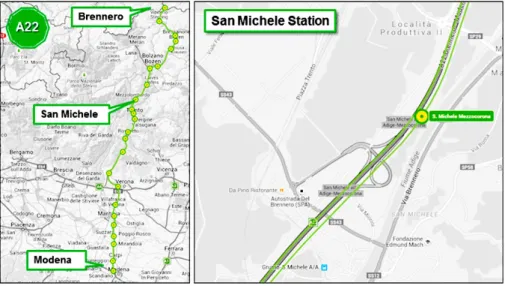
The most severe operating conditions of the infrastructure are related to the tourist flow peaks and so during these periods poor level of service or oversaturation conditions can be recorded. Together with these characteristics, we notice that A22 traffic is, in all its components, systematically growing consistent with the national freeway network trend. The Fig. 2.1 shows the S. Michele section of the A22 Freeway studied in this research.

(46)

Fig. 2.2. Analyzed section “S. Michele” at A22 Brenner Freeway

A22 Freeway sections ↓km↓ ↑km↑ City

Modena Nord 0 315

MO Campogalliano – Modena 3 311

Area Servizio "Campogalliano" 5 309 Carpi 11 303

Reggiolo 28 286 RE Pegognaga 37 277

MN Area Servizio “Po” 47 267

Mantova Sud 49 265 Mantova Nord 57 257

(47)

Area Servizio “Povegliano” 74 240 Verona Sud 86 228 Verona Nord 88 226 Area Servizio “Garda” 97 208 Affi – Lago di Garda Sud 98 207 Area Servizio “Adige” 119 186 Ala – Avio 135 179

TN Rovereto Sud – Lago di Garda Nord 147 167

Area Servizio “Nogaredo” 154 160 Rovereto Nord 156 158 Trento Sud 174 140 Trento Nord 182 132 Area Servizio “Paganella” 185 129 San Michele dell’Adige – Mezzocorona 193 121 Egna – Ora 212 102

BZ Area Servizio “Laimburg Ovest” - 99

Area Servizio “Laimburg Est” 218 - Bolzano Sud 229 85 Bolzano Nord 237 77 Area Servizio “Sciliar Ovest” - 69 Area Servizio “Isarco Est” 250 -

Chiusa – Val Gardena 261 53 Bressanone – Zona Industriale 266 48 Area Servizio “Plose” 272 42 Bressanone – Val Pusteria 276 38 Area Servizio “Trens” 294 20 Vipiteno – Barriera del Brennero 298 16

(48)

Area Servizio “Autoporto Sadobre” 298 16 Ponticolo - 7 Terme di Brennero - 5

Innsbruck – Confine di Stato – Austria 315 0 -

Table 2.1. Sections of the A22 Freeway

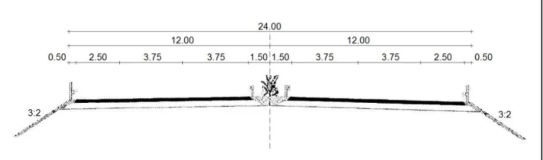
The infrastructure has a total length of about 313 km, has 2 lanes for each direction, each of a width of 3.75 m, hard shoulders of 2.50 m. The figure 2.3 below shows the road section of the A22 Freeway.

Fig. 2.3. Road section of A22 freeway.

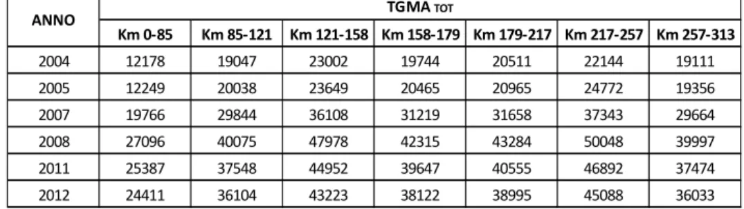
The most severe operating conditions experiencing low Service Levels or congested situations. Table 2.2 illustrates the traffic for the A22 wich exhibits systematic growth in accordance with the trend of the national highways.

(49)

The Average Annual Daily Traffic AADT (in Italian TGMA- Traffico Giornaliero Medio Annuo) is defined as the ratio between the number of vehicles traveling in a year and the number of days of the same.

Tab. 2.2. TGMAtot of A22 Freeway Northbound (Modena- Brennero)

Tab. 2.3. TGMAtot of A22 Freeway Southbound (Brennero- Modena) Km 0‐57 Km 57‐98 Km 98‐135 Km 135‐156 Km 156‐193 Km 193‐229 Km 229‐313 2004 19541 23277 20678 19988 23117 19775 11565 2005 19845 24985 21069 20657 23692 20139 12040 2007 30371 38237 32244 31617 36258 30821 18426 2008 40894 51485 43415 42566 48821 41499 24811 2011 38315 48238 40678 39882 45742 38882 23246 2012 36841 46383 39113 38348 43983 37387 22352 TGMA TOT ANNO Km 0‐85 Km 85‐121 Km 121‐158 Km 158‐179 Km 179‐217 Km 217‐257 Km 257‐313 2004 12178 19047 23002 19744 20511 22144 19111 2005 12249 20038 23649 20465 20965 24772 19356 2007 19766 29844 36108 31219 31658 37343 29664 2008 27096 40075 47978 42315 43284 50048 39997 2011 25387 37548 44952 39647 40555 46892 37474 2012 24411 36104 43223 38122 38995 45088 36033

(50)

Fig.2.4. TGMAtot of A22 Freeway Northbound (Modena- Brennero)

Fig. 2.5. TGMAtot of A22 Freeway Southbound (Brennero- Modena) 0 10000 20000 30000 40000 50000 60000 2004 ₂₀₀₅ 2007 ₂₀₀₈ 2011 ₂₀₁₂ TGMA TOT Year Km 0‐57 Km 57‐98 Km 98‐135 Km 135‐156 Km 156‐193 Km 193‐229 Km 229‐313 0 10000 20000 30000 40000 50000 60000 2004 ₂₀₀₅ 2007 ₂₀₀₈ 2011 2012 TGMA TOT Year Km 0‐85 Km 85‐121 Km 121‐158 Km 158‐179 Km 179‐217 Km 217‐257 Km 257‐313

(51)

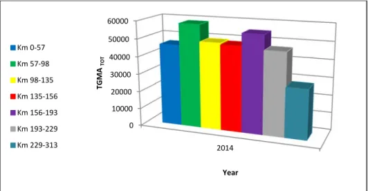
In addition, forecast of the traffic in the year 2014 was estimated (Tab. 2.4, 2.5 and Fig. 2.6).

Tab. 2.4. Prevision of TGMATOT in the year 2014 (Modena- Brennero)

Tab. 2.5. Prevision of TGMATOT in the year 2014 (Brennero- Modena)

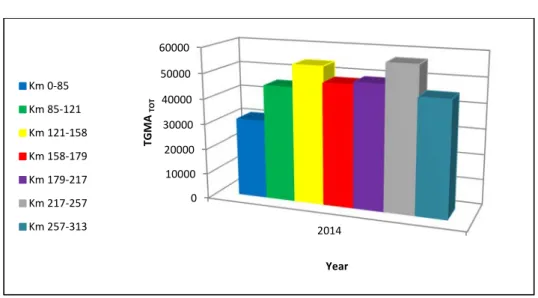
Fig. 2.6. Prevision of TGMATOT in the year 2014 (Modena- Brennero) Km 0‐57 Km 57‐98 Km 98‐135 Km 135‐156 Km 156‐193 Km 193‐229 Km 229‐313 2014 46157 58507 49024 48150 55168 46857 28091 TGMA TOT ANNO Km 0‐85 Km 85‐121 Km 121‐158 Km 158‐179 Km 179‐217 Km 217‐257 Km 257‐313 2014 30949 45165 54096 47902 48882 56943 45151

ANNO TGMA TOT

0 10000 20000 30000 40000 50000 60000 2014 TGMA TOT Year Km 0‐57 Km 57‐98 Km 98‐135 Km 135‐156 Km 156‐193 Km 193‐229 Km 229‐313

(52)

Fig. 2.7. Prevision of TGMATOT in the year 2014 (Brennero- Modena)

II.2 OVERWIEW OF THE CALIBRATION METHODOLOGIES

Before discussing in detail the recommended approach to the calibration and validation of micro-simulation models it is useful to state what exactly comprises “calibration” and “validation”:

 Model calibration is the process of tuning and refining the input data and parameters within the model in order to agree with real observed data, and thus provide a tool which is reliable for forecasting; 0 10000 20000 30000 40000 50000 60000 2014 TGMA TOT Year Km 0‐85 Km 85‐121 Km 121‐158 Km 158‐179 Km 179‐217 Km 217‐257 Km 257‐313

(53)

 Model validation is a process of comparing the results of the model with independent observed data.

In the transportation literature various methodologies for calibrating and validating traffic microsimulation models have been discussed in several publications (Barceló et al. (2010); Kim et al. (2005); Ma and Abdulhai (2002); Toledo et al. (2004); Park and Qi (2005); Abdalhaq and Baker (2014)).

Kim and Rilett (2003) applied a methodology that used a single measure, whereas other authors used more than one measure by executing sequences of calibration sub-processes, each one of which included different traffic measures for calibrating separate groups of parameters. Dowling et al. (2004b) proposed a three step methodology structured as follows: i) the calibration of the driving behavior parameters, performed by comparing capacities; ii) the calibration of the route choice parameters, performed by comparing flows; iii) and finally calibration completed by comparing travel times and queue lengths. Hourdakis et al. (2003) compared simulated and observed flows to calibrate global parameters such as maximum acceleration and other vehicle characteristics; then they compared simulated and observed speeds to calibrate local parameters and, finally, they proposed an optional calibration stage by comparing any measure chosen by the user. In order to find a set of model parameters that make the

(54)

model outputs as close as possible to the field-measured capacities, Dowling et al. (2004a) proposed that the capacity calibration was one of the steps in microsimulation calibration process. The calibration of the model to capacity consisted of the global calibration phase, performed to identify the appropriate network-wide value of the capacity parameters best reproducing on-field conditions, and the fine-tuning phase, performed so that the link-specific capacity parameters were adjusted to match more accurately the capacity measurements at each bottleneck. Queue discharge flow rate can be also used for the estimation of a numerical value for capacity, but loss of information can derive since the capacity should be expressed by a distribution of capacity values and not by a single numerical value only. In this regard, Brilon et al. (2007) introduced the stochastic approach for highway capacity analysis; thus, the capacity of a highway facility was regarded as a random variable instead of a constant value.

However, basing the capacity calibration process on a single numerical value, matching the means of the capacity distribution could not give very certain results, since other important properties of a distribution, or other traffic parameters characterizing capacity as speed or density, could be neglected (Menneni et al. (2008)). In any case, it should be noted that in the

(55)

calibration process, the main target should be to maximize the information suitable for replicating real system performances. Generalized relationships among speed, density, and flow rate can allow us to determine the required capacity information; these relationships can also provide information regarding free-flow and congested regions which cannot be gained from a single numerical value or a distribution of capacities. Based on speed-flow, speed-density, or flow-density relationships which provide information about the free-flow, congested, and queue discharge regions, a calibration procedure could replicate the whole range of traffic behavior and not just the peak period. For model calibration purposes, only a proportion of one of the three graphs mentioned above, instead of the entire graph, could be used (Menneni et al. (2008)). In any case, the amount of information available in fitting empirical/simulated data is very important, and more information can be obtained by using flow, speed-density, or flow-density graphs; as a consequence, a higher number of parameters can be submitted to the calibration process, resulting in a better fine-tuned simulation model. The calibration through speed-flow, speed density, or flow-density graphs could be considered as the first step, necessarily followed by route-choice and the system performance calibration. Despite the potential benefits in the calibration process, the use of the fundamental relationships of traffic flow in the microsimulation

(56)

calibration process remains still marginal. Wiedemann (1991) replicated field speed-flow relationships and used them to demonstrate closeness of field and simulated data; Fellendorf and Vortisch (2001) demonstrated the ability of a simulation model to replicate speed-flow graphs from real-world freeways. Menneni et al (2008) developed an objective function based on minimizing the dissimilarity between speed-flow graphs. Thus the dissimilarity of two graphs by calculating the amount of area that is not covered by the other was measured. Since speed and flow measurements were represented as point sets, discretization to convert point information to area was necessary. Moreover, considering that the information derived from the field and simulation was often just partial and not a complete speed-flow graph, the comparison was only made over the space occupied by the field graph. Differently from the approaches mentioned above, Mauro et al. (2014) developed the calibration methodology based on speed-density relationships in the microsimulation calibration process, stated that they represent the traffic-flow phenomenon in a wide range of operational conditions and well summarize all the information that may be collected in field (or following a run of the microsimulation model) on two of the three key variables of traffic flow. The matching of speed-density relationships from field and simulation

(57)

was evaluated using statistical analysis as a technique of pattern recognition.

II.3 THE FUNDAMENTAL DIAGRAM OF TRAFFIC FLOW

FOR THE A22 FREEWAY

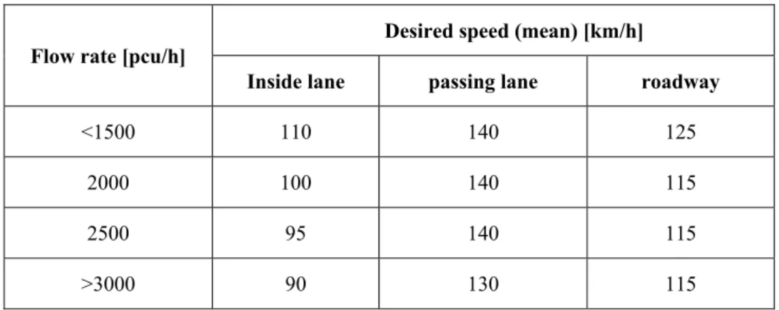
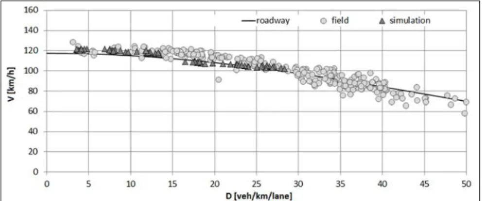
Experimental surveys carried out at observation sections on the A22 Brenner Freeway, Italy, have allowed the relationships between the fundamental variables of traffic flow (namely the speed-flow-density relationships) to be modelled for a traffic flow of cars only (Mauro 2003, 2005, 2007). Data were collected over different locations and multiple days and combined to show a complete graph between the pairs of traffic flow variables. The aforesaid relationships between flow and density, speed and density, speed and flow were developed for the right lane, the passing lane and the roadway, through the treatment and the processing of traffic data measured at specific observation sections (San Michele, Rovereto and Adige) on the A22 Freeway (Mauro 2003, 2005, 2007). A procedure for the estimation of the passenger car equivalent factors was also developed and reported in (Mauro 2003, 2005, 2007). For the same reference framework, under uninterrupted flow conditions an exploratory study proposed a criterion for predicting the reliability of freeway traffic flow by observing speed stochastic processes (see Mauro et al., 2013). First the relationship between speed and density was searched. This choice was motivated by the following: considering the real traffic flow phenomenon, the speed-density relationship is a monotonically