Asymptotic posterior approximation and efficient MCMC sampling for Generalized Linear Mixed Models

(1)

UC Irvine

UC Irvine Electronic Theses and Dissertations

Title

Asymptotic posterior approximation and efficient MCMC sampling for Generalized Linear Mixed Models Permalink https://escholarship.org/uc/item/03x8h0rt Author Berman, Brandon Publication Date 2019 License CC BY 4.0 Peer reviewed|Thesis/dissertation

(2)

UNIVERSITY OF CALIFORNIA, IRVINE

Asymptotic posterior approximation and efficient MCMC sampling for Generalized Linear Mixed Models

DISSERTATION

submitted in partial satisfaction of the requirements for the degree of

DOCTOR OF PHILOSOPHY in Statistics

by

Brandon Berman

Dissertation Committee: Wesley Johnson, Co-Chair Weining Shen, Co-Chair Michele Guindani

(3)

c

(4)

DEDICATION

To my family: My parents for their love and support from afar and over the years. My loving and supportive wife for all her help and patience over time.

(5)

LIST OF FIGURES

Page

2.1 History Plot for HDP Example . . . 22

2.2 MPSRF Plot for HDP Example . . . 23

2.3 Posterior Densities of Parameters in HDP Example . . . 26

2.4 Fitted Probabilities in HDP Example . . . 29

2.5 Posterior Densities for 90th percentiles in HDP Example . . . 31

2.6 Posterior Densities of Parameters whennp >2 . . . 34

2.9 Implementation of ARS Example . . . 43

2.10 Posterior Densities of Parameters for “Perfect” Data when (k, λ) = (300,25) 47 2.11 Posterior Densities of Parameters for “Perfect” Data when (k, λ) = (300,35) 47 2.12 Posterior Densities of Parameters for “Perfect” Data when (k, λ) = (300,50) 48 2.13 Posterior Densities of Parameters for “Perfect” Data when (k, λ) = (300,80) 48 2.14 Posterior Densities of Parameters for “Perfect” Data when (k, λ) = (300,100) 49 2.15 Posterior Densities of Parameters for “Perfect” Data when (k, λ) = (300,150) 49 2.16 Posterior Densities of Parameters for “Perfect” Data when (k, λ) = (300,200) 50 2.17 Posterior Densities of Parameters for “Perfect” Data when (k, λ) = (300,300) 50 2.18 Empirical CDF of nmin(p,1−p) values . . . 52

2.19 Posterior Densities of Parameters for Perfect Data when λ = 25 . . . 54

2.27 Example of Posterior Output with Standard Simulated Data . . . 61

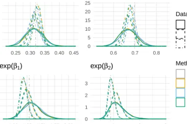
2.28 Posterior Densities for logit−1(β0) with Standard Simulated Data . . . 62

2.29 Posterior Densities for logit−1(β0 + 1.28σ) with Standard Simulated Data . . 63

2.30 Posterior Densities for exp(β1) with Standard Simulated Data . . . 64

2.31 Posterior Densities for exp(β2) with Standard Simulated Data . . . 64

2.32 Computation Analysis for Standard Simulated Data . . . 74

(9)

3.2 Covariates per hospital in HDP example . . . 99

3.3 History Plot for Extended HDP Example . . . 105

3.4 Posterior Densities of Parameters in Extended HDP Example . . . 107

3.5 Posterior Densities of Parameters in Extended HDP Example . . . 109

3.6 Posterior Densities of Parameters with Simulated Data . . . 133

4.1 Abortions per Herd . . . 163

4.2 Covariate Summaries in Cow Data . . . 164

4.3 MCMC History for Cow Abortion Example . . . 166

(10)

LIST OF TABLES

Page

2.1 Summary of HDP Data . . . 18

2.2 Posterior Results for HDP Example . . . 25

2.3 Fitted Probabilities Summary in HDP Example . . . 29

2.4 Results from HDP example . . . 31

2.5 Summary of Results with Standard Simulated Data, part 1 . . . 66

2.6 Summary of Results with Standard Simulated Data, part 2 . . . 67

2.7 Wall Time for “Perfect” Data . . . 72

2.8 Wall Time for Standard Simulated Data . . . 73

2.9 Average Wall Time, over k, for “Perfect” Data . . . 74

2.10 Average Wall Time, over λ, for “Perfect” Data . . . 75

2.11 Average Wall Time, over k, for Standard Simulated Data . . . 75

2.12 Average Wall Time, over λ, for Standard Simulated Data . . . 75

3.1 Summary of Covariates for HDP Example, expanded to include hospital level covariates (Chapter 3) . . . 97

3.2 Parameter Estimates and Quantities using HDP Data . . . 113

3.3 Summary of Results with Simulated Data . . . 143

3.4 Summary of Results with Simulated Data, part 2 . . . 144

(11)

List of Algorithms

Page 1 Pseudo Perfect Simulation Data . . . 40 2 Standard Simulated Data . . . 60 3 Data Simulation Mechanism . . . 132

(12)

ACKNOWLEDGMENTS

I would like to thank my colleagues, the faculty and staff in the statistics department at UC Irvine for the opportunity to learn and grow with them. I am especially thankful for professors Wes Johnson and Weining Shen for going above and beyond, and teaching me so much.

(13)

CURRICULUM VITAE

Brandon Berman

EDUCATION

Doctor of Philosophy in Statistics 2019

University of California, Irvine Irvine, CA

Bachelor of Arts in Mathematics 2010

California State University, Sacramento Sacramento, CA

Masters of Science in Civil Engineering 2005

University of California, Berkeley Berkeley, CA

Bachelor of Science in Structural Engineering 2004

University of California, San Diego La Jolla, CA

RESEARCH EXPERIENCE

Graduate Research Assistant 2018

TEACHING EXPERIENCE

Teaching Associate 2018

Teaching Assistant 2011–2018

PROFESSIONAL LICENSES

(14)

ABSTRACT OF THE DISSERTATION

Asymptotic posterior approximation and efficient MCMC sampling for Generalized Linear Mixed Models

By

Brandon Berman

Doctor of Philosophy in Statistics University of California, Irvine, 2019

Wesley Johnson, Co-Chair Weining Shen, Co-Chair

Generalized linear mixed models (GLMMs) provide statisticians, scientists, and analysts great flexibility to model data in a variety of situations. However, GLMMs frequently produce unrecognizable conditional distributions when attempting to analyze them in the Bayesian framework with Gibbs sampling. Traditionally, complex sampling schemes are used to ob-tain samples from these distributions. Our focus is to obob-tain asymptotic normal for these distributions and apply the theoretical results to speed up the process of MCMC.

(15)

Chapter 1 Introduction

Generalized linear mixed models (GLMMs) are among the most common tools used through-out statistics. They provide statisticians, scientists and analysts a unified modeling procedure to analyze a wide variety of scientific scenarios. GLMMs are complex despite their flexibility. They require complicated techniques to analyze. Throughout this thesis we demonstrate a methodology of how we can obtain inferences from using GLMM in an accurate and com-putationally efficient way.

In the first chapter we define generalized linear mixed models, discuss a common inferential technique in Bayesian methodology, and identify the problem we will discuss. In the following chapters we generalize to broader settings.

1.1 Generalized Linear Mixed Models

Generalized linear mixed models constitute a class of models. More importantly it is a class that is built upon the class of generalized linear models (GLMs).

(16)

1.1.1 Extending GLMs into GLMMs

To accurately describe a generalized linear mixed model one must first start with a general-ized linear model (GLM). According to McCullagh and Nelder [9], a GLM consists of three components:

1. A random component where the response variable is distributed as any member of the exponential family (more on this in a future section).

2. A systematic component where the (transformed) mean is modeled as a linear combi-nation of covariates.

3. A link function which connects the systematic and random components.

In addition to the three components GLMs make one major assumption: independence among the responses. This assumption is one of the principal shortcomings of the GLM. In longitudinal studies, the same observational unit is measured repeatedly across time leading to dependence in the observations. It is easy to imagine other situations where the independence assumption fails such as a familial study where all the observational units are people from the same family. Extending from the GLM class to the GLMM class is one way to eliminate independence assumption while keeping a similar structure.

The actual extension to GLMMs from GLMs is achieved by adding a random term within the systematic component. Typically the addition is done in a hierarchical fashion, that is, if Xiβ were the original systematic component then we would simply add a ui where ui

follows some distribution (though commonly assumed to be normally distributed) and the new systematic component would be Xijβ+ui. The change to the subscripts, adding j to i, is necessary to keep track of which observations belong to which clustering component. We typically use the convention that Xij is the covariate information for thejth observation

(17)

within theith_{cluster. Using this definition it is easy to recognize that the covariance between}

any two observations within the same cluster is not zero.

1.1.2 The Exponential Family

The exponential family, according to Casella and Berger [4], is a class of distributions where the pdf (or pmf) ofY can be expressed as:

f(y|θ) =h(x) exp η(θ)0T(y)−A(θ)

where θ is the vector of parameters and η, T are (possibly vector valued) functions, while A is the log-partitioning function. McCullagh and Nelder simplified this definition by rec-ommending that the parameters, θ, be transformed into their a canonical form so that η becomes the identity function and that the statistic T becomes the natural statistic. Under this parameterization, the pdf is expressible as:

f(y|θ) =h(y, φ) exp θy−b(θ) d(φ) .

Their version additionally introducesφ, the dispersion parameter, which may or may not be a constant.

One of the properties of the exponential family is that the results can be aggregated. Inde-pendent members of the exponential family with the same parameters are jointly distributed so their pdf, using the parameterization of McCullagh and Nelder, follows the following:

f(y|θ) = exp N X i=1 θyi−b(θ) d(φ) ! × N Y i=1 h(yi, φ).

Since the mean of the marginal distribution is ˙b(θ) (the derivative of b with respect to θ, evaluated atθ) then when aggregated, the estimator of the mean is the average,N−1PN

(18)

Under common assumptionsN−1PN

i=1yi is almost surely convergent to the mean ˙b(θ). Thus

when aggregated, there is a strongly consistent estimator for the canonical parameter.

Some members of the exponential family are already aggregated by definition. For exam-ple, the binomial distribution is the aggregated version of the Bernoulli distribution and the Gamma distribution, where the shape parameter is an integer, is the aggregation of exponen-tial distributions. In Chapters 2 and 3, we assume Bernoulli responses without information at the observational unit level. This makes it possible to use the aggregated version, i.e. the binomial distribution, to analyze the model. In Chapter 4, however, the response will remain Bernoulli, but with data at the observational unit level. This means we will not automatically have the built in strongly consistent estimator and additional justification will be needed.

1.2 Bayesian Analysis of GLMMs

In the previous section we discussed the details of generalized linear mixed models, but made no mention of how to go about carrying out inference on such a model. To this end, letYij be

the response of thejth _{observation in the} _ith_cluster,_X

ij the corresponding explanatory data

andui the random variable representing the effect of theith cluster. SinceYij is a member of

the exponential family, we let θ be the canonical parameter, but since it is a function of the systematic component, then we instead use θ(Xijβ+ui) to denote the response conditioned

upon the parameters. Thus the pdf is

f(yij|β, ui) = exp yijθ(Xijβ+ui)−b(θ(Xijβ+ui)) d(φij) h(yij, φij).

In the frequentist setting, the most common inferential method of inference is to maximize the likelihood function. However, when modeling a GLMM, the conditional pdf above is conditioned upon ui. We require an augmented data likelihood since ui is not observable.

(19)

The augmented likelihood is based on pretending that we were able to observe the random effect. We assume that the random effectuihas its own distribution with pdf g(ui|α). Then

the augmented likelihood is

L(β, u)≡ k Y i=1 ni Y j=1 f(yij|β, ui)×g(ui|α) = exp   X i,j yijθ(Xijβ+ui)−b(θ(Xijβ+ui)) d(φij)   " Y i g(ui|α) # Y i,j h(yij, φij)

Then we maximize the likelihood function with respect to both β and u.

Contrasting the frequentist approach, is the Bayesian approach. While there are much deeper philosophical connotations with both approaches, we note that the Bayesian approach assumes randomness about every quantity, but allows us to invoke Bayes theorem. In is most basic form Bayes theorem states:

P(B|A) = P(A|B)P(B)

P(A) .

Translating thisP(A|B) becomes the likelihood andp(B) the prior distribution andP(B|A) is the posterior distribution. Inferential quantities are based on posterior distributions. Let p(α, β) be the prior distribution forα and β. The posterior distribution in the GLMM case is: f(α, β,u|y) = Q i,jf(yij|β, ui)×g(ui|α)×p(α, β) R R Q i R Q jf(yij|β, ui)×g(ui|α)×p(α, β)duidα dβ

Since the integration in the denominator only produces a constant relative to the posterior density the denominator is ignored and the posterior is known only up to a constant.

f(α, β,u|y)∝Y

i,j

(20)

1.2.1 Gibbs Sampling

In order to draw inferences in the Bayesian setting requires full utilization the posterior distribution. However, since we do not typically carry out the integration in the denominator the posterior is only known up to a constant. The most common way to obtain estimates is with Monte Carlo techniques. Simply put, Monte Carlo techniques involve using a large sample from the posterior distribution, applying the inferential function to the samples and averaging the output. Now the issue is how to draw the samples.

The most common way to draw samples from an distribution that is known only up to a constant is with a Markov chain. We omit much of the technical definition of what a Markov chain is, but for this purpose, a Markov chain is a sequence of samples where the current sample depends only on the preceding one. To actually obtain a realization of a Markov chain an algorithm is needed. One of the most common choices for this is Gibbs sampling.

The Gibbs sampling algorithm is based on first obtaining the conditional distributions for each stochastic variable. Thus the critical step when using Gibbs sampling to carry out MCMC techniques using GLMMs is successfully obtaining these so called full conditional distributions. Full conditional densities are each proportional to the posterior density. Typ-ically, the conditional distributions are obtained by examining the posterior, isolating the terms that relate to the variable in question, and recognizing the result as a well known kernel. When the result is not a well known kernel then advanced techniques are needed such as slice sampling.

With GLMMs many of the conditional distributions are not recognizable; eg. when the kernel is not recognizable. Our methods asymptotics to approximate the portions of the resulting conditional density so that each conditional distribution is recognizable. This will result in a decrease in time necessary to construct the Markov chain and will make inferences easier to obtain.

(21)

1.3 Outline of the Thesis

The principal goal of the thesis is to first develop and then demonstrate our methods to a wider class of models as the thesis continues. In Chapter 2, we develop the methods and demonstrate the results for a GLMM model where the response is Bernoulli and the only explanatory information is within the cluster.

With a Bernoulli response there are two ways for the model to grow, either by an additional clustering level, or incorporating information for each observation. Both approaches present unique challenges for our methodologies that can be incorporated in future work. In Chapter 3, we focus on adding a layer to the model. In Chapter 4, we focus on the case when information is available for each response.

(22)

Chapter 2 Approximation to Binomial

Regression

2.1 Introduction

Generalized linear models (GLM) provide statisticians, scientists, and analysts great flexibil-ity to model data in a variety of situations. Perhaps the best argument in favor of generalized linear models is that they provide a universal framework for analyzing many different types of data. They allow a person with sufficient statistical knowledge the ability to model a multitude of continuous outcomes while using the same skill set to model a multitude of categorical outcomes. However, one of the limits of GLMs is that the original description of them provided by Nelder and Wedderburn (1972) [11] assumed independence among out-comes. That is to say GLMs are generally not able to accommodate longitudinal or repeated outcome data. An easy and common way to accommodate this situation is to expand the class of generalized linear models to generalized linear mixed models (GLMM) [10].

(23)

multiple observations per person or maybe several of the people are from the same familial group. In those scenarios there is a definite correlation among observations and the assump-tion of independence fails to hold. The advantage of the GLMM is that it maintains the universality of the generalized linear model but allows for correlation. This is accomplished by modeling in the GLMM setting the mean of the response variable as a linear combination of fixed and random effects. Including random effects creates a hierarchical aspect to the model and it allows for a correlation structure for repeated response or clustered data.

The additional hierarchical levels make fitting the model more complex. While there are models that allow for flexible distributions for random effects. Random effects are usually modeled with normal distributions for simplicity. We propose using large sample tech-niques, in conjunction with the normally distributed random effects to effectively approxi-mate GLMMs in a Bayesian setting, thus making it faster and more computationally efficient while maintaining accuracy.

In this chapter we focus on how to approximate a specific type of GLMM, namely binomial regression. We first derive the approximation in the first sections of this chapter. Later, we present an example of its use followed by simulations, which are used not only to illustrate the effectiveness and accuracy of the approximation, but also to show scenarios where our method breaks down. Following that we propose a solution that can further speed up our method.

2.2 Statistical Model, Priors, and Full Joint Posterior

We begin by discussing binomial regression where each observation contains its own random effect. Denote the data asY ={Yi: i= 1,2, . . . , k}and assume the model isYi

⊥

∼Bin(ni, pi)

(24)

independent and normally distributed with mean Xiβ and variance τ−1. The covariate

vector Xi is a row vector with the first entry 1 and with the remaining columns containing

the relevant covariates;βis a column vector of lengthprepresenting the fixed effect regression coefficients. Together these assumptions implyui

⊥

∼N(Xiβ, τ−1). Then the augmented data

likelihood is equal to k Y i=1 ni yi pyi i (1−pi)ni−yi r τ 2π exp −τ(ui−Xiβ) 2 2 ∝τk/2exp ( _k X i=1 yilogit(pi) +nilog(1−pi)− τ(ui−Xiβ)2 2 ) ∝τk/2exp ( _k X i=1 [yilogit(pi) +nilog(1−pi)]− τ(u−Xβ)0(u−Xβ) 2 ) (2.1) where u= (u1, u2, . . . , uk)0 and X = (X10, X 0 2, . . . , X 0 k) 0_.

In the Bayesian framework we assign prior probabilities toβand τ. One way to do that is to assume knowledge aboutβandτ can be reflected by the independent prior distributions,β ∼ Np(B0, C) and τ ∼ Gamma(a/2, b/2) where B0, C, a, b are hyper-parameters determined

by a priori knowledge. Consequently, the joint posterior for (β, u, τ) given the data is proportional to ∝τ(a+k)/2−1exp (" _k X i=1 [yiui−nilog(1 + exp(ui))] # − 1 2[τ(u−Xβ) 0 (u−Xβ) +(β−B0)0C−1(β−B0) +bτ ) (2.2)

The posterior in this case, like in many situations, is not recognizable so to make inferences requires Markov Chain Monte Carlo (MCMC) methods. MCMC methods are used to draw samples from the unknown joint posterior distribution, and thus are used to make inferences. Gibbs sampling is the typical method for implementation of MCMC techniques with GLMMs. Gibbs sampling requires the full conditional distributions for each block of parameters,u,β,

(25)

and τ. Subsequent repeated sequential sampling of these results in an MCMC sample from the joint posterior.

2.3 Full Conditional Distributions

To obtain these distributions we need to examine the joint posterior, Equation 2.2, with respect to each block while assuming the other blocks are fixed. The conditional distribution for u given everything else is

f(u|β, τ, y, X)∝exp ( _k X i=1 [yiui−nilog(1 + exp(ui))]− τ(u−Xβ)0(u−Xβ) 2 ) ∝exp ( _k X i=1 ni[˜πiui−log(1 + exp(ui))]− τ(ui−Xiβ)2 2 ) ∝ k Y i=1

exp{ni[˜πiui −log(1 + exp(ui))]}exp − τ 2 k X i=1 (ui −Xiβ)2 ! (2.3)

where ˜πi = yi/ni for all i. Observe that the ui’s are mutually independent, so we only

need to sample the marginal conditional distributions of the ui’s. Nonetheless, the density

function in Equation 2.3 is not recognizable. To sample from it requires advanced sampling techniques such as adaptive-rejection sampling or slice sampling, but such sampling increases the computational expense.

Examining Equation 2.2 we obtain the full conditional distribution for β

f(β|u, τ, y, X)∝exp −1 2 τ(u−Xβ)0(u−Xβ) + (β−B0)0C−1(β−B0) ∝exp −1 2 h τ(u−Xβ+Xβˆ−Xβˆ)0(u−Xβ+Xβˆ−Xβˆ) + (β−B0)0C−1(β−B0) i

(26)

where ˆβ = (X0X)−1_X0_u_{, assuming} _X0_X _{is non-singular. The purpose of introducing ˆ}_β _not

only facilitated the use of the complete the square formula, but it will in the future allow us a further simplification and ultimately a way to minimize computational time. In order to achieve this we recognize that

(u−Xβ)0(u−Xβ) = (u−Xβˆ+Xβˆ−Xβ)0(u−Xβˆ+Xβˆ−Xβ) =(u−Xβˆ) +X( ˆβ−β)

0

(u−Xβˆ) +X( ˆβ−β)

= (u−Xβˆ)0(u−Xβˆ) + ( ˆβ−β)0X0X( ˆβ−β) (2.4)

because the cross product term of (u−Xβˆ)0X( ˆβ−β) = 0. Continuing the derivation of the full conditional distribution for β, means that,

f(β|u, τ, y, X)∝exp n −τ 2(u−X ˆ β)0(u−Xβˆ)− τ 2(β− ˆ β)0X0X(β−βˆ) − 1 2(β−B0) 0 C−1(β−B0)

The preceding density is with respect to β, however, the term (u−Xβˆ)0(u−Xβˆ) does not involve β, thus, f(β|u, τ, y, X)∝exp −τ 2(β− ˆ β)0X0X(β−βˆ)− 1 2(β−B0) 0 C−1(β−B0) .

Utilizing the complete the square formula (see Section A.2) we simplify the density function,

f(β|u, τ, y, X)∝exp −1 2 β−(τ X0X+C−1)−1(X0uτ +C−1B0) 0 (τ X0X+C−1) × β−(τ X0X+C−1)−1(X0uτ +C−1B0) .

(27)

The preceding equation is the kernel of a multivariate normal density. Thus,

β|u, τ, y, X ∼ Np β∗,(τ X0X+C−1)−1

(2.5)

where β∗ = (τ X0X+C−1)−1(X0uτ +C−1B0). Similarly, the conditional distribution for τ

given everything else is

f(τ|β, u, y, X)∝τ(a+k)/2−1expn−τ

2[b+ (u−Xβ)

0

(u−Xβ)]o.

The preceding is the kernel of a Gamma density where the rate parameter is 0.5(a+k) and the shape parameter is 0.5[b+ (u−Xβ)0(u−Xβ)]. For the conditional distribution of β we introduced ˆβ and utilizing Equation 2.4 allows us to further simplify the shape parameter,

(u−Xβ)0(u−Xβ) = (u−Xβˆ)0(u−Xβˆ) + ( ˆβ−β)0X0X( ˆβ−β)

= (u−X(X0X)−1X0u)0(u−X(X0X)−1X0u) + ( ˆβ−β)0X0X( ˆβ−β) =u0(Ik−X(X0X)−1X0)u+ ( ˆβ−β)0X0X( ˆβ−β)

Hence, the full conditional for τ can be written as

τ|u, β, y, X ∼ Gamma a+k 2 , b+u0(Ik−X(X0X)−1X0)u+ (β−βˆ)0X0X(β−βˆ) 2 ! (2.6)

Thus, with Gibbs sampling and an additional advanced sampling technique we may utilize the conditional densities in Equations 2.3, 2.5, and 2.6 to obtain an MCMC sample.

2.4 Normal Approximation

As mentioned in the introduction of this chapter, the untapped benefit we are seeking is to combine the normal random effects distribution and a large sample theory result in order to

(28)

approximate the data augmented likelihood. Equations 2.1 and 2.3 are equivalent, however, one is the augmented data likelihood (2.1) wherein the later case, the formula is regarded as a function ofuwith the other parameters are fixed (2.3). Equation 2.3 along with Equations 2.5 and 2.6 are the full conditional distributions necessary for implementing a Gibbs sampler. As mentioned in Section 2.3, the conditional distribution in Equation 2.3 is not recognizable and would require additional techniques to sample from it. However if we give a normal approximation to Equation 2.3 then we should be able to save some computational effort without sacrificing much accuracy.

We propose to approximate the conditional distribution for u|β, τ, y, X, Equation 2.3, by using a Taylor series expansion. To that end, let hi: R → R where hi(ui) = ˜πiui −log(1 +

exp(ui)) for i = 1,2, . . . , k and ˜πi = yi/ni. To create second order Taylor series expansion

for hi we need the first and second derivatives ofhi

˙ hi(ui) = ˜πi− exp(ui) 1 + exp(ui) and ¨hi(ui) = − exp(ui) (1 + exp(ui))2 .

The “second order Taylor series expansion” forhi, centered at ˜ui, as defined by Ferguson [6],

is hi(ui) =hi(˜ui) + ˙hi(˜ui)(ui−u˜i) + (ui−u˜i)2 Z 1 0 Z 1 0 s¨hi(˜ui+rs(ui −u˜i))dr ds.

If we let ˜ui = logit(˜πi) then ˙hi(˜ui) = 0. Summing over i k X i=1 nihi(ui) = k X i=1 ni[˜πiui−log(1 + exp(ui))] = k X i=1 ni hi(˜ui) + (ui−u˜i)2 Z 1 0 Z 1 0 sh¨i(˜ui+rs(ui−u˜i))dr ds .

However, since ¨hi is a continuous function and ˜πi a.s.

−→ pi as ni → ∞ for each i then by the

continuous mapping theorem ˜ui a.s.

(29)

Recall that by definition ui = logit(pi) and so ˜ui−ui a.s.

−→ 0 and ˜ui+rs(ui−u˜i) a.s −→ ui =

logit(pi) as ni → ∞, for any r, s∈[0,1]. Note that ¨hi is always non-negative and bounded

by 0.25, so the integral is subject to the Dominated Convergence Theorem, DCT, that is,

Z 1 0 Z 1 0 s¨hi(˜ui+rs(ui−u˜i))dr ds a.s. −→ 1 2 ¨ hi(logit(pi)) =− pi(1−pi) 2

as ni → ∞. The difference is o(1) almost surely. Moreover,

Z 1 0 Z 1 0 s¨hi(˜ui+rs(ui−u˜i))dr ds+ ˜ πi(1−π˜i) 2 =op(1) since ˜πi a.s. −→pi. Thus, since √ n(˜ui−ui) = Op(1) then ni(ui−u˜i)2 Z 1 0 Z 1 0 s¨hi(˜ui+rs(ui−u˜i))dr ds+ ˜ πi(1−π˜i) 2 =Op(1)·op(1) =op(1)

Returning to the summation over i, then since ˜πi a.s. −→pi (asni → ∞), k X i=1 nihi(ui) = k X i=1 ni hi(˜ui) + (ui−u˜i)2 Z 1 0 Z 1 0 sh¨(˜ui+rs(ui−u˜i))dr ds − (ui−u˜i) 2_π_˜ i(1−π˜i) 2 + (ui−u˜i)2π˜i(1−π˜i) 2 = k X i=1 nihi(˜ui)− k X i=1 ni(ui−u˜i)2π˜i(1−π˜i) 2 + k X i=1 ni(ui−u˜i)2 Z 1 0 Z 1 0 s¨h(˜ui+rs(ui−u˜i))dr ds+ ˜ πi(1−π˜i) 2 = k X i=1 nihi(˜ui)− k X i=1 ni(ui−u˜i)2 ˜ πi(1−π˜) 2 +op(1)

(30)

by Slutsky’s theorem. Thus we approximate Equation 2.3 with f(u|β, τ, y, X)∝exp ( −1 2 k X i=1 (ui−u˜i)2niπ˜i(1−π˜i) +τ(ui−Xiβ)2 ) (2.7)

Equation 2.7 is useful since the complete the square formula could be used to combine the two quadratic terms involving ui. A cleaner approach would be to state the equation in

a multivariate form and then complete the square. Since we already defined u equal to (u1, u2, . . . , uk)0 then we can similarly define ˜u = (˜u1,u˜2, . . . ,u˜k)0. Let Dnπ˜(1−π˜) be a k×k

diagonal matrix where Dnπ˜(1−π˜) = diag{niπ˜i(1−π˜i) : i = 1,2, . . . , k}. Then equation 2.7

becomes approximately f(u|β, τ, y, X)∝exp −1 2 (u−u˜)0Dnπ˜(1−π˜)(u−u˜) +τ(u−Xβ)0(u−Xβ)

Completing the square using formula (see A.2) gives

f(u|β, τ, y, X)∝exp −1 2 u−(Dnπ˜(1−π˜)+τ Ik)−1(Dnπ˜(1−π˜)u˜+τ Xβ) 0 ×(Dnπ˜(1−π˜)+τ Ik) u−(Dn˜π(1−˜π)+τ Ik)−1(Dn˜π(1−π˜)u˜+τ Xβ)

which is the kernel of ak dimensional multivariate normal density. Hence

u|β, τ, y, X ∼· Nk (Dnπ˜(1−π˜)+τ Ik)−1(Dnπ˜(1−π˜)u˜+τ Xβ),(Dnπ˜(1−π˜)+τ Ik)−1

(2.8)

2.5 Data Analysis

At this point, we can sample from the approximate joint posterior distribution using Gibbs sampling. Sampling the conditional distributions presented in Equations 2.3, 2.5, and 2.6 gives an exact Gibbs sampler, but 2.3 is not a known density and would require additional

(31)

sampling techniques. Our method simply substitutes Equation 2.8 for Equation 2.3.

To explore the quality of this approximation we used data from the University of Califor-nia, Los Angeles’s Institute of Digital Research and Education (IDRE). This institute is a collaboration across different departments within that university whose goal is to assist researchers, and one such group within the institute is dedicated to statistics and data in-formatics. The statistics and data informatics group assists researchers through in-person and online consulting. In fact, the group’s statistical presence is a well-known resource for statistics help.

The data we are using to demonstrate our method is the IDRE’s hospital, doctor, and patient (HDP) dataset. The dataset is a rich collection of data with multiple hierarchical levels with many different facets. To explore our method, we use the data to model the probability of a physician’s ability to facilitate lung cancer remission using only physician level covariates. There are 308 oncology physicians in the dataset who have treated 6745 individuals for lung cancer. Since we are limited to physician level covariates the only available covariates are the physician’s years of experience, the number of malpractice lawsuits involving the physician, and whether or not the physician attended a top ranked medical school.

The number of years a physician has been practicing is an important covariate; the more experience a physician has, ideally, the better the treatment. The number of malpractice lawsuits may have a negative effect on the probability of a physician’s ability to successfully facilitate cancerous tumor remission, as it may be viewed as a sign of carelessness. However, in a litigious society, a malpractice lawsuit can be filed over a trivial cause. There are no additional details explaining the types of lawsuits in these data.

The model that we propose involves Yi, the number of patients that physician i treated

(32)

Table 2.1: Summary of Covariates for HDP Example Covariate Mean (SD) Years of Experience 17.96 (4.08) Number of Lawsuits 1.97 (1.53) Med. School Top 69 (22.4%) Avg 239 (77.6%)

treated. Our model specifies Yi

⊥

∼ Bin(ni, pi) wherepi = logit(ui) and

ui

⊥

∼ N β0+β1Xexperience,i+β2Xlawsuits,i+β3Itop med. school,i, τ−1

for i= 1,2, . . . ,308.

Table 2.1 provides a summary of the covariate information. For convenience in the prior specification, we actually use standardized continuous covariates meaning that Xexperience is

the quantity (years of experience−mean years of experience)/SD(years of experience), and similarly for the number of lawsuits variable. Of course, we do not standardize the indicator variable.

2.5.1 Elicitation of the prior for the example

In order to use the proposed methodology, we must specify priors for the parameters. The prior distribution for β is specified as a particular multivariate normal distribution and a gamma distribution onτ. The prior we specify will be rather diffuse but not overly so. While we prefer informative priors, there is really very little prior information available to us for this particular situation.

Generally, the prior would be elicited with the assistance of a subject-matter expert or by one’s own information that is external to the data. In this example, however, we do not have

(33)

access to an expert and are relatively uninformed about successes in an oncological setting. To make sense of this we begin by applying diffuse priors that will not overly effect the posterior. As previously mentioned, we start by standardizing the experience and number of lawsuits within our data. This allows us to relate the intercept parameter to the probability of success. A physician with 18 years of experience and approximately 2 lawsuits, and who did not attend a top medical school, is the baseline observational unit and in this case, E(ui) = β0. Thus conceptually we can think about the probability of cancer remission for

patients under this type of physician’s care. We naively suppose that the best guess for such an oncologist is 50%.

We know that our prior contains only information about an oncologist’s skill and not the patient’s condition or other unaccounted for covariates, so we need to incorporate this un-certainty into our model. If we are 95% certain that the typical physician (the one with 18 years of experience, was involved in 2 malpractice suits, and attended an average medical school) will have a cancer remission rate, sayp, between 10% and 90%, and if our best guess for pis 50%, we have logit(0.5) = 0, and logit(0.1) =−logit(0.9) = −2.2, so,

0.95 = Pr(0.1≤p≤0.9) = Pr(logit(0.1)≤logit(p)≤logit(0.9))

= Pr(−2.2≤β0 ≤2.2) = Pr −2.2−0 σ ≤Z ≤ 2.2−0 σ

where Z is the standard normal distribution and where we have assumed β0 ∼ N(0, σ2).

From elementary statistics we can find a value ofσ by realizing that 2.2/σ= 1.96 orσ = 1.1. Thus a reasonable prior for β0 isN(0,1.21) (1.12 = 1.21), since logit(0.5) = 0.

We could repeat this process, specifying a prior distribution for the rest of theβ coefficients. Since we are unsure of ourselves, our best guess for a physician’s probability for cancer remission could be 50%, namely this leads to the thought that E(u) = E(Xβ) = 0 across all covariate vectors. This is accomplished by setting the mean of the prior forβ to be a vector

(34)

of zeroes. The variance components for the prior on β is a larger challenge.

The assumption of independence is quite useful to handle the variance component; it results in zero values for the covariance terms in the normal prior forβ. This is a common assump-tion. Furthermore, since we standardized the continuous covariates so that they are on a similar scale, it is not unreasonable to assume roughly the same amount of uncertainty for each of the coefficients. This assumption means we can use a linear combination correspond-ing to an extreme case to find a value of the variance. Suppose we are 95% certain that the probability of remission for the most successful type of physician, that is the one who has the most experience (Xexperience = 2.75), fewest lawsuits (Xlawsuits = −1.25) and attended a

top medical school, is between 0.1 and 0.9 then we can use similar reasoning to find a value of the variance of β. We obtain

0.95 =P(−2.2≤β0+ 2.75β1−1.25β2+β3 ≤2.2) =P ₋ 2.2−0 √ σ2_{+ 2}_.₇₅2_σ2_{+ 1}_.₂₅2_σ2₊_σ2 ≤Z ≤ 2.2−0 √ σ2_{+ 2}_.₇₅2_σ2_{+ 1}_.₂₅2_σ2 ₊_σ2

where each β ∼ N(0, σ2). Then solving _σ√ −2.2

2+2.752₊₁_.₂₅2 =−1.96 yieldsσ =

−2.2

−1.96√2+7.5+1.5 =

0.34. Thus our guess for the variance component of β is between 0.34 and 1.21. Taking the largest value is the most conservative option, but results in a more diffuse prior. Taking the smallest value utilizes the limited information we have. An acceptable compromise between these extremes is to assume thatσ = 1. Furthermore, Christensen et al (2010) [14] commonly use standard normal priors for binomial regression coefficients under these circumstances. Thus the prior on β is,

β ∼ N3(B0 = 0, C =I3).

The prior used for τ is a gamma distribution. A common distribution used to model the precision is the chi-square distribution with one degree of freedom. Since the gamma distri-bution is a generalized version of the chi-square distridistri-bution then the prior that we use for

(35)

τ is

τ ∼ Gamma(1/2,1/2).

2.5.2 Results

In order to test our methodology, we used the priors derived in Section 2.5.1. Our first goal was to insure convergence of Markov chains using our method. We ran the chain for 5000 iterations and discarded the initial 10% of it as burn-in. We initially ran the code with three chains to check for convergence, Figure 2.1 shows the history plots of the three chains thinning every other iteration to compensate for graphical limitations. For the purposes of illustration, two of the physicians were randomly selected and the history of ufor those two physicians is also included. Figure 2.2 is a plot of the multivariate potential scale reduction factor (MPSRF) using Brooks and Gelman’s method[1]. Smaller values, closer near 1, are indicative of the chains mixing well, that is, the chains are more similar than not. Based on Figures 2.1 and 2.2 we believe that the chains are converging to the same values.

We now compare our method of Gibbs sampling with a normal approximation to the method used in JAGS. Both methods used the same prior, the same number of iterations and the same burn-in. To compare results, we plot smoothed histograms of estimated odds ratios and estimated probabilities. In Figure 2.3 we present five quantities: logit−1(β0), logit−1(β0 +

1.28σ), exp(β1), exp(β2), and exp(β3). The quantity logit−1(β0) represents the probability

of a “typical” physician, one with approximately 18 (17.96) years of experience, subject to approximately 2 (1.97) lawsuits, and did not attend a top ranked medical school, to remit a patient’s cancerous tumor. The 18 years of experience, 2 lawsuits, and matriculation from an average medical school, are not random- these are the values that correspond to the mean covariate values. Since the quantitative covariates are standardized in the model this would imply values of 0 for the typical physician’s covariates. For the medical school covariate, we

(36)

u280 β4 σ u127 β1 β2 β3 1000 2000 3000 4000 5000 1000 2000 3000 4000 5000 1000 2000 3000 4000 5000 1000 2000 3000 4000 5000 1000 2000 3000 4000 5000 1000 2000 3000 4000 5000 1000 2000 3000 4000 5000 −0.5 0.0 0.5 −2 −1 0 1 0.0 0.2 0.4 0.6 0.9 1.0 1.1 1.2 1.3 1.4 −1.0 −0.8 −0.6 −0.4 −0.4 −0.2 0.0 0.2 0.0 0.5 1.0 1.5 2.0 Iteration V alue chain 1 2 3

Normal Appx History Plot

Figure 2.1: History plots for parameters using the Normal Approximation in HDP Example

coded average medical school as zero and top-ranked medical school as one. Thus even the medical school covariate for the typical physician is zero. The logit−1(β0 + 1.28σ) quantity

represents the 90th percentile of cancer remission probability for the typical physician. This

means that for all physicians with baseline (which we deemed “typical”) covariate values that 90% of them have success probabilities of patient remission below this value.

The other objects of interest, exp(β1), exp(β2), and exp(β3), are estimated odds ratios with

each one corresponding to one of the three covariates included in the model. For example, exp(β1) corresponds to the estimated odds ratio comparing the ability of a physician, with

four more years of experience (or one additional standard deviation), to the ability of another physician, with the same education attainment level and number of lawsuits, to place a patient’s tumor into remission. The quantity exp(β2), like exp(β1), is also an estimated

odds ratio, but corresponds to the number of lawsuits covariate. In this odds ratio, we are comparing the estimated odds of cancer remission for patients who were attended by two

(37)

1.25 1.50 1.75 1000 2000 3000 4000 5000 Iteration R p ^

R

^

p

Multivariate PSRF

Figure 2.2: Plot of Multivariate Potential Scale Reduction Factor (MPSRF) using Brooks and Gelman’s method.

physicians, both with the same amount of experience and both attending a medical school of similar prestige, but one physician was involved in approximately one and half more lawsuits than the other. The final estimated odds ratio, exp(β3) corresponds to the medical

school covariate. It compares the estimated odds of cancer remission for two physicians with a similar number of malpractice lawsuits and experience, but one attended a top ranked medical school while the other one attended an average ranked one. In addition to these five quantities, Figure 2.3 also includes an empirical CDF of the estimate nimin(pi,1−pi)

values. This graph will be important in further discussion.

In addition to Figure 2.3 we provide Table 2.2 to display the numerical summaries associated with the posterior distributions for the objects of interest. In particular, the smoothed histogram for the posterior distribution of exp(β1) and its corresponding summaries show

that the median of the odds ratio under normal approximation as 1.31 with 95% PI of (1.12,1.53). This means that if there two physicians of equal education and number of lawsuits, but one physician has four more years of experience, that on average, the physician with four of more years of experience has odds of tumor remission that are 31% higher than

(38)

the less experienced physician. The same odds ratio is estimated to be 1.34 using JAGS with a 95% PI of (1.13,1.58). These medians and 95% PI only differ slightly and when comparing odds, such minor differences are trivial unless the reference odds are disproportionately small or large.

This minor discrepancy that exists between estimated odds ratios is also present in exp(β2)

and exp(β3) as well. For exp(β2) the estimated odds ratio is 0.86 with a 95% PI of (0.60,1.21)

with our normal approximation and 0.84 with a 95% PI of (0.58,1.22) with JAGS. The interpretation of these results is that, under the normal approximation, the estimated odds of a patient’s cancer remission when treated by a physician with one standard deviation more lawsuits (approximately 1.5 lawsuits) are about 14% lower than they would be when treated by a physician with similar experience and medical education, but fewer lawsuits. This negative result coincides with what we hypothesized, that lawsuits do negatively impact, but not overtly so, a physician’s ability to successfully treat a cancerous tumor.

Similarly, for exp(β3), the estimated odds ratio is 0.92 with a 95% PI of (0.78,1.08) under

the normal approximation and 0.91 with a 95% PI of (0.76,1.08) under JAGS. This means that the estimated odds of a patient’s cancer remission would be approximately 8% lower (9% under JAGS) when treated by a physician who attended a top ranked medical school compared to a physician who did not attend a top ranked medical school, given that both physicians have the same experience and were subject to the same number of lawsuits. The fact that the difference in the median is only 1% between the two methods is good evidence that our method can be a good approximation of JAGS.

None of the odds ratios varied greatly when estimated under normal approximation versus under JAGS. In fact, for the odds ratios, the posterior density curves are nearly identical under both methods. However, to understand odds ratios one needs to know something about the reference odds. To find the reference odds the baseline probability must be cal-culated first. For the typical physician, the one with 18 years of experience, involved in two

(39)

lawsuits and did not attend a top ranked medical school, the estimated probability of cancer remission for a patient is 0.34 and 0.32 using normal approximation and JAGS, respectively, with associated 95% PIs of (0.30,0.38) and (0.28,0.36). These estimates and probability intervals are derived from the posterior distribution of logit−1(β1). Note the discrepancy of

0.02 is observable in Figure 2.3 with the posterior density of logit−1(β1) under the normal

approximation being greater than the same density under JAGS. However, this discrepancy is relatively minor and the estimated medians and 95% PIs are similar to each other. Fur-thermore, the estimated probabilities would produce an estimate for odds of a patient’s cancer remission for a typical physician to be about 0.52 using normal approximation and 0.48 using JAGS. The associated 95% PI for the odds would be (0.43,0.61) under normal approximation and (0.39,0.56) under JAGS.

With an estimate for the reference odds of cancer remission for the typical physician we are better able to understand the estimated odds ratios. For example, the odds of cancer remission for a physician who had four additional years of experience but was otherwise a “typical” physician can be approximately estimated as 0.52×1.31 = 0.68 under normal approximation and 0.48×1.34 = 0.63 under JAGS. These estimated odds, like the estimated odds ratios, are very similar which is indicative that the normal approximation method we proposed can replicate the results from JAGS.

Parameter Method 2.5%tile Median 97.5%tile Mean SD exp(β1) Normal Appx 1.12 1.31 1.53 1.31 0.10 JAGS 1.13 1.34 1.58 1.34 0.12 exp(β2) Normal Appx 0.60 0.86 1.21 0.87 0.15 JAGS 0.58 0.84 1.22 0.86 0.16 exp(β3) Normal Appx 0.78 0.92 1.08 0.92 0.08

JAGS 0.76 0.91 1.08 0.91 0.08 logit−1(β0)

Normal Appx 0.30 0.34 0.38 0.34 0.02 JAGS 0.28 0.32 0.36 0.32 0.02

Table 2.2: Posterior Inferences for the HDP example

In Table 2.2 and Figure 2.3, notice that the results using our proposed methodology are remarkably close to those for JAGS. We presented odds ratios for the three covariates

(40)

in-0 5 10 15 20 0.25 0.30 0.35 0.40

logit

−1

(

β

0

)

0 5 10 15 0.60 0.65 0.70 0.75 0.80

logit

−1

(

β

0

+1.28

σ

)

0 1 2 3 4 0.9 1.1 1.3 1.5 1.7

exp(

β

1

)

0 1 2 0.4 0.6 0.8 1.0 1.2 1.4

exp(

β

2

)

0 1 2 3 4 5 0.7 0.8 0.9 1.0 1.1 1.2

exp(

β

3

)

0.00 0.25 0.50 0.75 1.00 5 10 15

E. CDF of posterior np values

Method Normal Appx JAGS

Comparing Methods with HDP Dataset

Estimated Value

Est. Density

Figure 2.3: Posterior density plots using HDP data with JAGS and Gibbs Sampling with Normal Approximation. logit−1(a) = (1 + exp(−a))−1_.

(41)

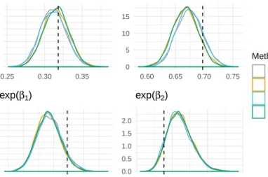
cluded in our study along with the probability of cancer remission for the typical physician. However there is a curiosity that occurs when discussing the 90th _{percentile of cancer}

re-mission for the typical physician. The smoothed histograms of the posterior densities for logit−1(β0+ 1.28σ) show the density (more appropriately, the mode of the density) for the

normal approximation to be less than that for JAGS. In table 2.4, the estimated 90th

per-centile for the probability of cancer remission for the typical physician is 0.68 with a corre-sponding 95% PI of (0.63,0.73) using normal approximation and 0.70 with a corresponding 95% PI of (0.65,0.75) under JAGS. Thus there is also a difference of 0.02 between the two methods. We observed a similar difference of 0.02 when discussing the posterior densities of logit−1(β0), however, in that case, the estimated probability was lower using JAGS than

it was using the normal approximation, the opposite of what we observe in the posterior density of logit−1(β0 + 1.28σ).

We included the 90th percentile for typical physicians in order to convey information

re-garding σ, the standard deviation of the random effect. Figure 2.3 shows the normal ap-proximation mirroring the results of JAGS for the odds ratios quantities. This means the discrepancy of 0.02 between these posterior densities is due to the differences in how β0 is

estimated, while the switching is due to how σ, the standard deviation is estimated.

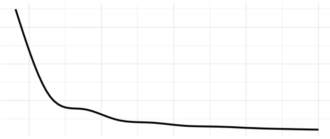
Since our method is effectively based on the normal approximation to the binomial we decided to pursue a deeper understanding of the approximation. In elementary statistics, the approximation of the binomial distribution by the normal distribution is appropriate whennmin(p,1−p) exceeds a certain threshold; Cochran [5] does not recommend an explicit threshold value, but does recognize the threshold is typically set at 5 or 10. However, Cochran suggests that in situations like this where we are attempting to “summarize knowledge in a specific situation” that there is no all encompassing solution.

Following this advice we created the empirical CDF of the posterior medians fornmin(p,1− p). We created the empirical CDF by transforming the posterior iterates for the random

(42)

effect, u, via the inverse logit (expit) function to the probability scale for each physician at each iteration of the Markov chain. Then we obtained the median of the fitted probabilities thus obtaining an estimate of the probability of cancer remission for each physician. Finally, by multiplying the number of patients each physician has attended to and the minimum of the estimate of this probability and one minus the estimated probability we can order the values and create an empirical CDF. The resulting plot is seen in Figure 2.3. What we learned from this plot is that a significant portion of the data would fail to meet the typically used criteria to justify a normal approximation to a binomial distribution; approximately 50% of the physicians have an estimatednmin(p,1−p) value that is less than 5 and almost 90% of the physicians have an estimated nmin(p,1−p) value that is less than 10.

So far the results are encouraging. The normal approximation produces estimates for quan-tities of interest that are similar to JAGS. But the results also raised some interesting ques-tions regarding the estimation of the standard deviation of the random effect. The precision corresponding to the standard deviation is one of the conditional distributions within the Gibbs sampler. The conditional distribution of the precision depends on the iterates of u. Thus we need to investigate those samples. In the next section, we continue the investiga-tion, by diving in deeper and investigate the values u. We will examine some of the results for different physicians followed up by an examination into the 90th _{percentile quantity,}

logit−1(β0+ 1.28σ).

2.5.3 Results, part II

In augmented likelihood models the random effect is often a nuisance, but in this example the random effect, u, is the logit of the probability of cancer remission for each physician. It is conceivable that there might be interest in the value of u, or more appropriately, the probability itself. Since there are 308 physicians in the dataset, we randomly selected two

(43)

Physician 171 Physician 218 Physician 4 Physician 116 0.0 0.2 0.4 0.6 0.5 0.6 0.7 0.8 0.9 1.0 0.0 0.2 0.4 0.6 0.2 0.4 0.6 0.8 0 1 2 3 4 0 2 4 6 8 0 5 10 0 2 4

Est. Fitted Probability

Est. Density

type

Normal Appx JAGS

Fitted Probabilities for Four Physicians

Figure 2.4: Fitted Probability Densities for Four Select Physicians in HDP example

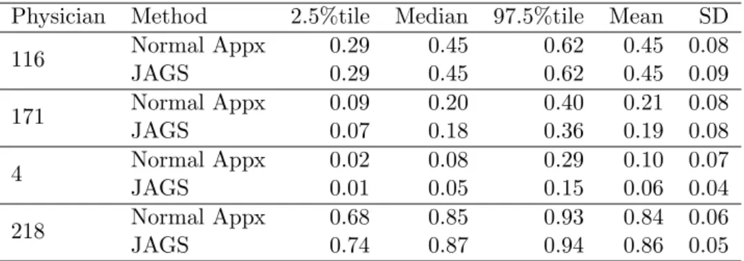
Physician Method 2.5%tile Median 97.5%tile Mean SD 116 Normal Appx 0.29 0.45 0.62 0.45 0.08 JAGS 0.29 0.45 0.62 0.45 0.09 171 Normal Appx 0.09 0.20 0.40 0.21 0.08 JAGS 0.07 0.18 0.36 0.19 0.08 4 Normal Appx 0.02 0.08 0.29 0.10 0.07 JAGS 0.01 0.05 0.15 0.06 0.04 218 Normal Appx 0.68 0.85 0.93 0.84 0.06 JAGS 0.74 0.87 0.94 0.86 0.05

Table 2.3: Summary of Fitted Probabilities for Four Select Physicians in HDP example

physicians. In addition to the randomly selected physicians we selected the two physicians with the most extreme naive estimates of the probability of cancer remission; we selected the physicians with the smallest and largest yi/ni values. For these physicians, we give

the estimated probability of cancer remission both graphically (Figure 2.4) and numerically (Table 2.3). Physicians 116 and 171 are the randomly selected ones, while Physician 218 had the largestyi/ni value and Physician 4 had the smallest yi/ni value. In both Figure 2.4 and

Table 2.3 the estimates for the probability of cancer remission for Physicians 116 and 171 are nearly identical for both methods, however the results for Physicians 4 and 218 are noticeably different. The tails of these densities are definitely larger using the normal approximation

(44)

method, but the medians are similar. It is worth noting that Physician 4 only treated one patient out of 34 patients successfully while Physician 218 successfully treated 36 out of 40 patients. These two physicians are exceptional cases where their data do not conform well to a normal approximation, even under the loosest criteria. However, for physicians not in the extremes, like Physician 116 and 171, who successfully treated 14 out of 30 and 4 out of 22 patients, respectively, our normal approximation method appears to successfully mimic JAGS.

Finally, we present the posterior for logit−1(β0 + 1.28σ) and for logit−1(β0 +β1 + 1.28σ),

which are the 90th _{percentile of cancer remission for typical physicians and for physicians}

who are 1 standard deviation, approximately four more years, more experience than average, respectively, graphically (Figure 2.5) and numerically (Table 2.4). We discuss inferences for these two physicians to gauge impact of experience and to assess the effect of σ on the accuracy of the normal approximation relative to JAGS.

Previously, we noted the smoothed histogram for the 90th percentile of cancer remission for

the typical physician is lower using the normal approximation that it was under JAGS. This same fact, the smoothed histogram being greater under JAGS than normal approximation, occurs in the 90th _{percentile of cancer remission for the physician who was involved in 2}

lawsuits, did not attend a top ranked medical school, and has 22 years of experience. Table 2.4 reinforces this observation: the median for the logit−1(β0+1.28σ) is 0.68 with a 95% PI of

(0.63,0.73) under normal approximation but 0.70 with a 95% PI of (0.65,0.75) under JAGS. The median for logit−1(β0+β1+ 1.28σ) is 0.73 with a 95% PI of (0.68,0.79) under normal

approximation and 0.76 with a 95% PI of (0.70,0.81) under JAGS. Thus both percentiles differ by about 0.02 under the normal approximation versus under JAGS.

However, there is an additional piece of information gleaned by examining the change in the median and the 95% PI in logit−1(β0 + 1.28σ) versus logit−1(β0 +β1 + 1.28σ). When

(45)

Average Experience 0.5 0.6 0.7 0.8 0.9 0 5 10 15 Four Additional Years of Experience 0.6 0.7 0.8 0.9 0 5 10 15 type Normal Appx JAGS

90th Percentile of Fitted Probabilities for an Average Physician

Est. Fitted Probability

Est. Density

Figure 2.5: Posterior densities for logit−1(β0 + 1.28σ) and logit−1(β0+β1+ 1.28σ) in HDP

Example where logit−1(a) = (1 + exp(−a))−1.

approximately 0.05 lower for the 90th _{percentile of cancer remission for typical physicians}

than they are for physicians who have 22 years of experience, did not attend a top ranked medical school and were involved in 2 lawsuits. The same change of about 0.05 is observed when examining the medians and 95% PI under JAGS. Since the same effect is observed under both methods then the estimation of σ is the problem. Further, if σ is estimated correctly by JAGS then the estimation by the normal approximation is too low. This implies that our samples from the conditional distribution of τ are too large, which occurs if we are not sampling from the correct conditional distribution of u. Since ui = logit(pi) then we know

which conditional distribution needs to be examined.

90th percentile for the

Method 2.5%tile Median 97.5%tile Mean SD of cancer remission

for physician

Average Experience Normal Appx 0.63 0.68 0.73 0.68 0.02 JAGS 0.65 0.70 0.75 0.70 0.02 Four additional Normal Appx 0.68 0.73 0.79 0.73 0.03 years of experience JAGS 0.70 0.76 0.81 0.76 0.03

Table 2.4: 90th percentile of the probability of successfully treating a tumor for selected physicians comparing Gibbs sampling with a normal approximation and JAGS.

(46)

2.5.4 Discussion of the Example

Our results so far have issues that require discussion, first, the data are not true data; the UCLA IDRE generated the data using specific criteria related to an investigation. Thus, no conclusion regarding an oncology physician’s ability to treat a patient can be drawn using these data. Furthermore, as previously mentioned, the capability to put a patient’s can-cer into remission heavily depends on the patient’s presenting symptoms, can-certainly factors unique to each patient such as the location, size, and possible metastasization of lung cancer affect the physician’s ability to successfully treat a patient. Regardless of the lack of scientific importance, there is an interesting statistical outcome. The proposed methodology of in-corporating a normal approximation within a Gibbs sampler appears to perform reasonably well.

In our example, we were interested in showing that by using a normal approximation within the Gibbs sampler is equivalent to using the current standard Bayesian statistical tool, JAGS. Our normal approximation performed well when estimating β but did not perform as well when estimatingσ. For estimating the physician’s probability of cancer remission the normal approximation performed better when the data for the physician is sufficiently large. We suspect that if all the physicians’s data were sufficiently large our estimates our estimates for ui would be better, and in turn, our estimate for σ would become indistinguishable for

the two methods. In the next section we investigate this claim.

2.5.5 Exploring The Results

When examining the results of the HDP example, Sections 2.5.2 and 2.5.3, we saw that our method of approximation performed reasonably well. However, the results were not perfect as discussed in those sections. Figure 2.4 showed good results for physicians who were not at the extremes. This is due to the fact that the data for those physicians conformed to the

(47)

normal approximation to the binomial.

Our first attempt to resolve this issue involved considering only the physicians who had treated more than 10 patients. But this attempt did not resolve the issue. The heart of the matter is that we are attempting to use a normal distribution to approximate an unknown, but albeit, a log concave distribution, Equation 2.3. This unknown distribution’s density is obtained as the product of binomial and normal densities, thus the normal approximation is only about the binomial part. If the normal approximation to the binomial is good then our approximation will be good.

We address issues about treating the discrete, binomial distribution as a continuous, normal distribution. Cochran [5] suggests that a discrete distribution can be approximated by a normal distribution when the expected counts in each cell exceed 5 or 10, but warns that rigid adherence to such doctrine might be harmful. If we filter our data on the basis of the expected counts and then run the same experiment as before, then we might eliminate our discrepancies. The summary of our experiment is: (1) Run JAGS code using the prescribed prior and the full dataset, run only one chain with a small number of iterations, say B iterations. For each of the 308 physicians in the data set, calculate the expected counts. That is, from each of the B draws from u|β, τ, y, X, obtain nimin(pij,1−pij), where j

is the jth _{iteration (out of} _B _iterations), _i _{is the} _ith _{physician, and} _u

ij = logit(pij). (2)

For each of the i physicians calculate the median value across the B iterations, namely, calculate medianj∈B{nimin(pij,1−pij) : i= 1, . . . ,308}. (3) Create a subset of the original

data by using only the physician’s whose median value exceeds some threshold. (4) Repeat the analysis using the defined subset. By including only physicians whose data conforms better to the normal approximation we can achieve better results.

Setting the threshold value to 1 results in an unique situation. All 308 physicians have a mediannmin(p,1−p) value greater than 1. Figures 2.6, 2.7, and 2.8 show the output from this experiment when the threshold value is set to 2, 5, and 10, respectively. Each figure

(48)

displays (i) the fitted probability of cancer remission corresponding to an “typical” (18 years of experience, did not attend a top ranked medical school, and was involved in two lawsuits) physician (logit−1(β0)), (ii) the 90th percentile for the probability of cancer remission for a

typical physician, (iii) the odds ratio for cancer remission corresponding to a physician with an additional four years of experience (exp(β1)), (iv) the odds ratio involving physicians

with one and a half additional lawsuits (exp(β2)), and (v) the odds ratio for physicians who

attend a top medical school versus one who attended an average medical school (exp(β3)).

In addition we provide the empirical CDF of the posterior median nmin(p,1−p) values.

0 5 10 15 20 0.30 0.35 0.40 0.45

logit

−1

(

β

0

)

0 5 10 15 0.65 0.70 0.75 0.80

logit

−1

(

β

0

+1.28

σ

)

0 1 2 3 4 1.00 1.25 1.50

exp(

β

1

)

0 1 2 0.4 0.8 1.2 1.6

exp(

β

2

)

0 1 2 3 4 5 0.8 1.0 1.2 1.4

exp(

β

3

)

0.00 0.25 0.50 0.75 1.00 5 10 15

E. CDF of posterior np values

Comparing Methods with Subset of Physician Dataset

n min(p,1−p) > 2

Estimated Value

Est. Density

Figure 2.6: Estimated Conditional Densities based on data with Expected Count >2

In Figure 2.6 we display the same results as Figure 2.3 except restricted the data to cases where nmin(p,1− p) exceeds 2. For the each of the odds ratios there is no discernible difference when comparing the JAGS and normal approximation methods. However, there is a noticeable difference for the probability of cancer remission for the typical physician and

(49)

for the corresponding 90th _{percentile for probability of cancer remission when comparing the}

densities under the JAGS and normal approximation methods. Thus Figures 2.6 and 2.3 are very similar. The lack of a difference between these two figures indicates that subsetting the data based on nmin(p,1−p) > 2 is not a stringent enough threshold. Based on the empirical CDF in Figure 2.3, approximately 25% of the data fails to meet the threshold. The corresponding empirical CDF in Figure 2.6 is for the remaining 246 conditions and as such should be regarded as a conditional CDF.

0 5 10 15 0.40 0.45 0.50 0.55

logit

−1

(

β

0

)

0 5 10 15 0.65 0.70 0.75 0.80

logit

−1

(

β

0

+1.28

σ

)

0 1 2 3 1.0 1.2 1.4 1.6

exp(

β

1

)

0 1 2 3 0.6 0.9 1.2 1.5

exp(

β

2

)

0 1 2 3 4 0.8 1.0 1.2 1.4

exp(

β

3

)

0.00 0.25 0.50 0.75 1.00 5.0 7.5 10.0 12.5 15.0 17.5

E. CDF of posterior np values

Comparing Methods with Subset of Physician Dataset

n min(p,1−p) > 5

Estimated Value

Est. Density

Figure 2.7: Estimated Conditional Densities based on data with Expected Count >5

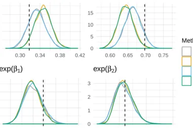
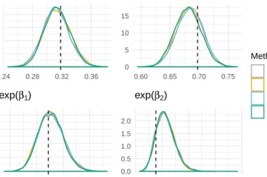
Since the results of our experiment were not satisfactory we continue the experiment by increasing the threshold value to 5. Results can be seen in Figure 2.7. The most striking observation is that by having nmin(p,1−p) > 5 the density of the probability of cancer remission for the typical physician is approximately the same using both the normal approx-imation method and JAGS. This contrasts with what we saw in Figures 2.3 and 2.6 where

(50)

the densities for the probability of cancer remission for the typical physician differed between the two methods. In addition, there are subtle changes within the odds ratio densities. The two methods generate similar density curves, but the mode of the curves changes as the data changes.

Increasing the threshold to 5 did not resolve everything; the densities for the 90th _percentile

for the probability of cancer remission for the typical physician are still somewhat different for the two methods. Since we are working on the assumption that the difference in the densities is due to the normal approximation to the binomial distribution then we may need to further increase the threshold value.

Increasing the threshold value needs to be done carefully, only 138 physicians are left when the threshold value is 5. The empirical CDF shows that approximately 25% of these 138 physicians have mediannmin(p,1−p) values less than 7.5 and approximately 75% have me-dian values less than 10. The value of 10 is tempting, many statisticians use the requirement that nmin(p,1−p) be greater than 10 to be large enough to treat a binomial distribution as a normal distribution.

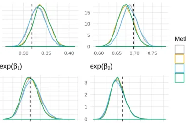
When we increased the threshold to 10 we were left with only 38 physicians out of the original 308. While there are clear issues with discarding almost 90% of the data it did provide an attractive result: there is almost no discernible difference between the normal approximation method and JAGS when it comes to the densities of the parameters. Even the densities for both methods of the 90th percentile are virtually indistinguishable. However

inferences based on different “cherry picked” subsets of data can be radically different. Just compare the modes of the density curves in the Figures 2.3, 2.6, 2.7 and 2.8. For example the mode of logit−1(β0) is less than 0.35 in Figure 2.3, but is nearly 0.5 in Figure 2.8. Similarly,

the odds ratio, exp(β3) goes from 0.91 to being greater than 1.

Asymptotic posterior approximation and efficient MCMC sampling for Generalized Linear Mixed Models

UC Irvine

UC Irvine Electronic Theses and Dissertations

DEDICATION

TABLE OF CONTENTS

LIST OF FIGURES

LIST OF TABLES

List of Algorithms

ACKNOWLEDGMENTS

CURRICULUM VITAE

Brandon Berman

ABSTRACT OF THE DISSERTATION

Chapter 1

Introduction

1.1

Generalized Linear Mixed Models

1.1.1

Extending GLMs into GLMMs

1.1.2

The Exponential Family

1.2

Bayesian Analysis of GLMMs

1.2.1

Gibbs Sampling

1.3

Outline of the Thesis

Chapter 2

Approximation to Binomial

Regression

2.1

Introduction

2.2

Statistical Model, Priors, and Full Joint Posterior

2.3

Full Conditional Distributions

2.4

Normal Approximation

2.5

Data Analysis

2.5.1

Elicitation of the prior for the example

2.5.2

Results

Normal Appx History Plot

R

^

Multivariate PSRF

logit

(

β

)

logit

(

β

+1.28

σ

)

exp(

β

)

exp(

β

)

exp(

β

)

E. CDF of posterior np values

Comparing Methods with HDP Dataset

2.5.3

Results, part II

Fitted Probabilities for Four Physicians

2.5.4

Discussion of the Example

2.5.5

Exploring The Results

logit

(

β

)

logit