Simulation and Framework for the Humanoid Robot TigerBot

RIT Scholar Works

RIT Scholar Works

8-2018

Simulation and Framework for the Humanoid Robot TigerBot

Simulation and Framework for the Humanoid Robot TigerBot

[email protected]

Follow this and additional works at: https://scholarworks.rit.edu/theses

Recommended Citation Recommended Citation

Sze, Felisa, "Simulation and Framework for the Humanoid Robot TigerBot" (2018). Thesis. Rochester Institute of Technology. Accessed from

This Thesis is brought to you for free and open access by RIT Scholar Works. It has been accepted for inclusion in Theses by an authorized administrator of RIT Scholar Works. For more information, please contact

Simulation and Framework for the Humanoid Robot

TigerBot

by

Felisa Sze

A Thesis Submitted in Partial Fulfillment of the Requirements for the Degree of Master of Science in Electrical Engineering

Supervised by Professor Dr. Ferat Sahin

Department of Electrical and Microelectronic Engineering Kate Gleason College of Engineering

Rochester Institute of Technology Rochester, New York

August 2018

Approved by:

Dr. Ferat Sahin, Professor

Thesis Advisor, Department of Electrical and Microelectronic Engineering

Dr. Gill Tsouri, Associate Professor

Committee Member, Department of Electrical and Microelectronic Engineering

Dr. Sohail A. Dianat, Professor

Dedication

I dedicate this thesis to my family for their support, and especially to my sister for her encouragement.

Acknowledgements

I would like to thank Dr. Ferat Sahin for advising and supporting me through this project. I also want to thank my colleagues in the MABL group, both alumni and newcomers, for their support and understanding as well.

Abstract

Simulation and Framework for the Humanoid Robot TigerBot Felisa Sze

Supervising Professor: Dr. Ferat Sahin

Walking humanoid robotics is a developing field. Different humanoid robots allow for different kinds of testing. TigerBot is a new full-scale humanoid robot with seven degrees-of-freedom legs and with its specifications, it can serve as a platform for humanoid robotics research. Currently TigerBot has encoders set up on each joint, allowing for position control, and its sensors and joints connect to Teensy microcontrollers and the ODroid XU4 single-board computer central control unit. The components’ communication system used the Robot Operating System (ROS). This allows the user to control TigerBot with ROS. It’s important to have a simulation setup so a user can test TigerBot’s capabilities on a model before using the real robot. A working walking gait in the simulation serves as a test of the simulator, proves TigerBot’s capability to walk, and opens further development on other walking gaits. A model of TigerBot was set up using the simulator Gazebo, which allowed testing different walking gaits with TigerBot. The gaits were generated by following the linear inverse pendulum model and the basic zero-moment point (ZMP) concept. The gaits consisted of center of mass trajectories converted to joint angles through inverse kinematics. In simulation while the robot follows the predetermined joint angles, a proportional-integral controller keeps the model upright by modifying the flex joint angle of the ankles. The real robot can also run the gaits while suspended in the air. The model has shown the walking gait based off the ZMP concept to be stable, if slow, and the actual robot has been shown to air walk following the gait. The simulation and the framework on the robot can be used to continue work with this walking gait or they can be expanded on for different methods and applications such as navigation, computer vision, and walking on uneven terrain with disturbances.

List of Contributions

• Implemented position control on the real robot using ROS

Contents

List of Figures ... viii

List of Tables ... ix

Chapter 1: Introduction ... 1

Chapter 2: Literature Survey ... 3

2.1 Overview of Humanoid Robots ... 3

2.2 Overview of Humanoid Robotics Concepts ... 5

2.2.1 ZMP ... 6

2.2.2 LIPM ... 7

2.2.3 Alternate Walking Methods ... 10

Chapter 3: TigerBot Overview ... 15

3.1 Introduction ... 15

3.2 TigerBot Anatomy ... 16

3.3 TigerBot Electronics and Software ... 19

Chapter 4: TigerBot Simulation ... 24

4.1 Creating a URDF ... 24

4.2 MoveIt! ... 27

4.3 Gazebo ... 29

4.3.1 Gazebo Overview ... 29

4.3.2 Gazebo and ROS ... 31

4.4 Running the Walking Gait ... 33

4.4.1 Standing ... 33

4.4.2 Walking Gait Generation ... 34

4.4.3 Gait Execution using ROS ... 46

Chapter 5: Using the Real Robot to Air-Walk ... 48

Chapter 6: Results ... 51

6.1 Simulation Results ... 51

Chapter 7: Conclusion ... 59 Chapter 8: Future Work ... 60 Bibliography ... 62

List of Figures

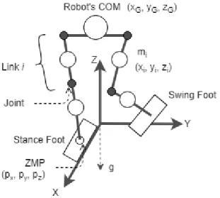
Figure 1: Diagram of a generic robot labeled with common terminology. ... 5

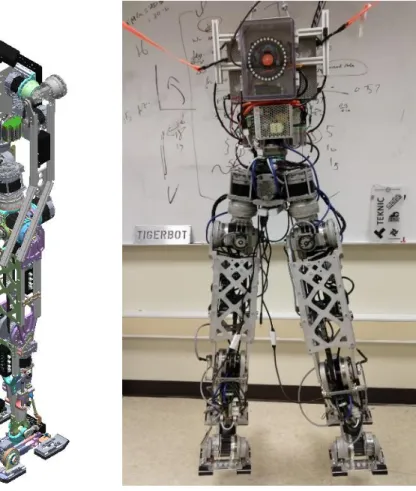
Figure 2: TigerBot, as (a) a SolidWorks model and (b) the physical build. ... 15

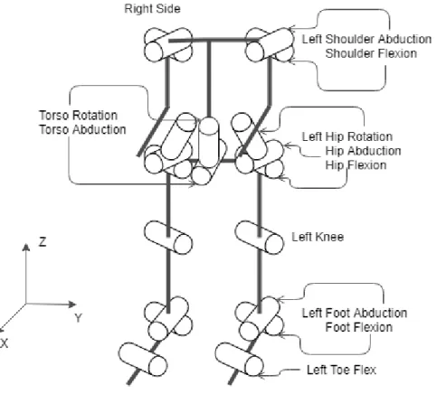
Figure 3: Joints of TigerBot and world frame ... 16

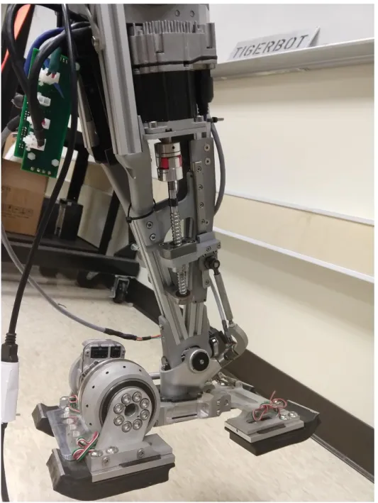
Figure 4: Picture of TigerBot’s right ankle ... 18

Figure 5: Picture of PCB stack ... 20

Figure 6: Flowchart of communication between hardware ... 21

Figure 7: TigerBot’s collision model ... 26

Figure 8: TigerBot in RViz using MoveIt! ... 28

Figure 9: TigerBot in Gazebo ... 30

Figure 10: ROS node graph for the simulation ... 33

Figure 11: LIPM COM trajectory graph ... 35

Figure 12: Theoretical used walking gait graph ... 39

Figure 13: Flowchart for the walking simulation program ... 42

Figure 14: Flowchart for air-walking ... 49

Figure 15: ROS node graph for air-walking ... 50

Figure 16: Simulated walking gait graph ... 53

Figure 17: Close up of simulated walking gait graph ... 54

Figure 18: Theoretical and simulated walking gait graph overlaid ... 54

Figure 19: Comparision of TigerBot in standing pose (a) Simulation (b) Real robot ... 55

Figure 20: Comparision of TigerBot in initial leaning to right pose (a) Simulation (b) Real robot ... 56

Figure 21: Comparision of TigerBot after stepping with left foot (a) Simulation (b) Real robot ... 56

Figure 22: Comparision of TigerBot in leaning to left pose (a) Simulation (b) Real robot ... 57

Figure 23: Comparision of TigerBot after stepping with right foot (a) Simulation (b) Real robot ... 57

Figure 24: Comparision of TigerBot in leaning to right pose (a) Simulation (b) Real robot ... 58

List of Tables

Table 1: Characteristics of TigerBot ... 17 Table 2: The parameters of the simulation walking gait ... 39 Table 3: The data from the simulated walking gait... 51

Chapter 1: Introduction

Humanoid robotics is an important field. Robots that mimic the human form and move and walk like humans can access spaces meant for humans and lead to improvements in prosthetics and other forms of robotics connected to humans. Humanoid walking robots, for example, would be able to access the different terrains humans can, like stairs. Like other legged robots, bipedal robots could navigate rough terrain, and full-scale humanoid robots can navigate on eye-level with humans. Humanoid robots are well suited for interacting with humans since they can fit in spaces other mobile robots might not, and with arms and end-effectors, can use devices as a human would.

Many humanoid robots have been developed, both small-scale and full-scale. Since the WABOT series of robots from Waseda University, humanoid robots have expanded in complexity, versatility, and robustness, being able to walk, run, recover from disturbances, navigate on their own, and more. Once companies and research facilities build appropriate humanoids, they can be used to research different methods for movement and applications for humanoid robots.

TigerBot is a new full-scale humanoid robot from Rochester Institute of Technology. It was intended to be a tour guide for RIT visitors, and is currently a platform for graduate students to test humanoid applications such as walking. It has 7 degrees of freedom per leg, including an active toe, and sensors such as encoders, force sensors, and an IMU. Built as it is, it should be capable of balancing and walking. Simulation allows walking gaits to be tested on a model before testing the gaits on the real robot.

A simulation model of TigerBot was constructed using the simulator Gazebo with the Robot Operating System (ROS). To prove its usability, a working walking gait was generated and tested to work with TigerBot. The walking gait involved generating inverse kinematics using MoveIt! based off the desired center-of-mass (COM) trajectory. The trajectory was designed to keep the

zero-moment-point within the support polygon outlined by the robot’s feet while switching the COM between each foot to allow the swing foot to lift and take a step. The gait is mainly in the double support phase for stability, which allows the simulated robot to walk hundreds of steps before falling. There is also fall-resistance and recovery based on the COM’s velocity.

The real TigerBot is suspended on an engine hoist, allowing for air-walking. The single-board computer and the microcontrollers distributed on TigerBot were programmed for position control to follow the control scheme set up in the simulation, and the walk gait was given to the robot for it to perform, which it did adequately. This set up can be reused should the simulation be expanded on, or act as a basis for other forms of control.

Past this introduction, this thesis delves into other humanoid robots designed in the past and humanoid walking concepts. It then covers TigerBot and its hardware and software features. The software that was set up for simulation is explained, and the progress of the walking gait and how it runs in simulation follows. Then how the real TigerBot is set up for control is covered, and how might its capability as a platform for future students be expanded.

Chapter 2: Literature Survey

2.1 Overview of Humanoid Robots

The first full-scale humanoid robot capable of walking was WABOT-1 in 1973 from Waseda University. It was followed by WABOT-2 in 1984. Honda created a series of humanoid robots; P2 in 1996 was able to walk. It had successors P3, in 1997, and ASIMO, in 2000. Following these initial robots came other walking humanoid robots such as HRP-2, JOHNNIE, KHR-2, Nao, and LOLA.

Honda’s ASIMO is one of the well-known early walking humanoid robots. Its predecessor, P2, had 6 degrees-of-freedom (DOF) per leg and 7 DOF arms, with force sensors on the feet and a ground inclination sensor. It walked using the ZMP concept, and can correct its posture using sensors, allowing for walking on inclines [1]. ASIMO is similar to P2, though it has modified 6 DOF arms. It also had vision and auditory systems for navigation and human communication [2].

HRP-2 came from Japan’s Humanoid’s Robotics Project in 2002. It had standard 6 DOF legs and arms, and also waist joints. It could walk on rough terrain without tipping over, and could recover from a fall [3].

KHR-2 is the successor to KHR-1, coming from Korea Advanced Institute of Science and Technology. It has 41 DOF total including 11 DOF arms and hands, and six DOF legs. It walks following a pattern alternating between single and double support phases. It uses dampening control during the single support phase, landing orientation and timing control during the transition between phases, and ZMP control during the double support phase to keep the ZMP at the center between the feet. During the walking pattern, the torso’s roll and pitch are controlled to keep the torso upright using an inertia sensor in the torso and the ankle’s pitch joint and the pelvis’s position [4].

NAO is a small, affordable humanoid robot from the company Aldebaran-Robotics. It walks using ZMP and an open-loop walking algorithm. It also has a unique hip design where the pelvis is made up of two angled hinged joints with a single motor opposed to a waist joint and the two hip rotation joints [5].

TigerBot is heavily inspired by the humanoid robot LOLA [6]. LOLA is a full scale bipedal robot with 7 DOF legs and 3 DOF arms, and is the successor to JOHNNIE, both of which come from the Technical University of Munich. LOLA has been used as a platform for fast walking, obstacle avoidance, dynamic walking, and more [7] [8] [9].

LOLA was modeled in a dynamic simulation with consideration towards rigid multibody dynamics, contact dynamics, and drive dynamics. The rigid multibody dynamics were described with equations of motion that were calculated by considering the robot made up of multiple rigid links, with different masses. The contact dynamics described the feet’s contact with the ground; this is necessary as LOLA has shock absorbing material on the soles of its feet. The drive dynamics concern the permanent magnet synchronous motors used on LOLA. Assumptions are made to model them as dc motors, to then get the actuator torque. These equations are combined to have equations for the entire robot’s dynamics [10].

For walking, LOLA uses a real-time walking pattern generator to generate a COM trajectory from desired footstep locations. Walking parameters are used to calculate constraints, which go towards foot trajectories. These trajectories are converted into contact torque reference trajectories, which can be converted to ZMP. The COM x and y axis trajectories are then generated based on these trajectories, and on assuming a modified LIPM where the mass of the robot is split into three points for the torso and each leg. This is done instead of the traditional LIPM with a single mass since with a faster walking speed, the swing foot motion becomes more influential to the COM

trajectory [11]. LOLA also has stabilization in a form of impedance control. The concept is hybrid force and position control along with a joint position control loop and a contact force trajectory control loop [10].

LOLA’s sensor system includes absolute encoders for the joints, force/torque sensors for the feet, and an IMU in the chest. The control system was made up of a central control unit housed in the chest connected to nine smaller control units for lower-level tasks. The central control unit handled walking on its own, but an external computer was used for monitoring and sometimes vision. It also used an external power supply [10].

2.2 Overview of Humanoid Robotics Concepts

This section covers terminology and concepts used in humanoid robotics research. This includes the zero-moment point, the linear inverse pendulum model, and other methods of bipedal walking. Some terms and variables are shown in Figure 1, to illustrate what they refer to.

2.2.1 ZMP

One common walking method is through zero-moment point (ZMP) control. The ZMP is the point where the net horizontal (x and y directions) moments from ground forces and the ankle forces is zero, leaving the vertical reaction forces and momentum at that point. [12].

ZMP as a concept came from Vukobratovic and Juricic [13] who also suggested using it in gait synthesis. It was first used practically with the WL-10RD robot in 1984, at Waseda University [12].

For a biped robot consisting of multiple links, ZMP can be approximated as:

𝑝

=

𝑝

=

Where px and py are the x and y coordinates of the ZMP (with the x-y plane being the ground plane), xi, yi, and zi are the coordinates of the center of mass (COM) for a particular link i for each approximate link of the robot, and mi is the mass of the link i [14]. These terms and locations are illustrated in Figure 1.

In the single stance, the ZMP should be located within the supporting foot, the shape of it being the support polygon; in the double stance, it should be within a support polygon bounded by the robot’s feet. For dynamic equilibrium, the ZMP should be in the support polygon. Should the ZMP approach and leave the support polygon edge, the robot will tilt around that edge and fall. The control system should then keep the ZMP in the support polygon, keep it from getting to close to the edge of the support polygon, and avoid loss of equilibrium due to disturbances.

The ZMP coincides with the center of pressure (COP) when the robot has a dynamically balanced gait, but the center of pressure is not always the ZMP, which happens when the gait is not dynamically balanced and the ZMP does not exist [12].

The COM of the robot is also linked to the ZMP. When the ZMP is at the edge of the support polygon, the robot begins to tip in that direction. But the COM can leave the support polygon if its dynamically balanced, with the ZMP still within the polygon. A walking gait can then be generated by moving the COM forward while keeping it supported. One way to do so is to model the legs and the COM as inverse pendulums, often called the linear inverse pendulum model (LIPM) [14].

2.2.2 LIPM

The LIPM models the robot as a single mass point at the robot’s COM. The COM represents the mass of the linear inverse pendulum, and the end of the pendulum is located at the ZMP. The model also assumes the ZMP can be approximated by the supporting foot’s placement, centered underneath the foot’s ankle. With this model, the ZMP and the COM are related to each other by:

𝑥

̈ =

𝑧_𝐺

(𝑥

− 𝑝

∗

₎

Where xG and its double derivative is the position and acceleration of the COM along the x-axis (considered to be the axis of the robot’s trajectory, shown in Figure 1), p*x is the ZMP location along the same axis, zGis the height of the COM, and g is gravity. The perpendicular axis y follows the same equation.

Assuming the ZMP to be constant under the supporting foot, the analytical solutions for the trajectory of the inverse pendulum is [14] [15]:

𝑥(𝑡) = (𝑥

− 𝑝

) cosh (

) + 𝑇

𝑥

̇

𝑠𝑖𝑛ℎ (

) + 𝑝

𝑥̇(𝑡) =

sinh (

) + 𝑥

̇

𝑐𝑜𝑠ℎ (

)

𝑇

= √

Where xi(n) and x˙i(n) are the initial location and velocity of the COM along the x-axis at the start of the n-th step, t is time, and p*x is the x component of the ZMP, or foot location [15].

The trajectory of the inverse pendulum that makes up a step is called a walking primitive. The walking primitive spans a time range from zero to Ts, where Ts is the time it takes for a step in the single support phase. Walking primitives can be linked together to form a piece-wise function for a rudimentary walking gait if the final positions and velocities of the previous primitive match that of the initial positions and velocities of the next primitive [14] [15].

These equations and required constraints for consecutive steps lead to other equations detailing the final position and velocity of the COM for each primitive and individual foot placement. To get specific foot placement for the desired final COM positioning an evaluation function for the error between the desired and real COM positions and velocities is minimized as much as possible, leading to the foot placement to reduce desired COM position error [14].

The evaluation function is:

𝑁 = 𝑎(𝑥

_{− 𝑥}

)

+ 𝑏(𝑥̇

_{− 𝑥}

̇

)

Where a and b are positive weights, xdand 𝑥̇𝑑_{are the desired COM position and velocity, and x}n f and 𝑥̇_𝑓𝑛 are the final COM position and velocity of the n-th step. It is desired for N to be zero, so the way to do that would be to make xf equal xd.

To use the evaluation function, xf is needed. It can be determined from a state-space variation of equations 4 and 5:

[

𝑥

𝑥

̇ ] = [

𝐶

𝑇

𝑆

𝑆/𝑇

𝐶

] [

𝑥

𝑥

̇ ] + [

1 − 𝐶

−𝑆/𝑇

] 𝑝

Where C is cosh(t/Tc) and S is sinh(t/Tc), xn

fand 𝑥̇_𝑓𝑛 are the final COM position and velocity of the n-th step, xniand 𝑥̇_𝑖𝑛 are the initial COM position and velocity of the n-th step, p*x is the ZMP’s x-component, and Tc comes from equation 6.

By inserting the xn

f and 𝑥̇_𝑓𝑛 determined from equation 8 into equation 7 and solving for the ZMP’s x component, p*x, comes the optimized foot placement function:

𝑝

= −

(𝑥

_{− 𝐶𝑥}

_{− 𝑇}

𝑆𝑥

̇

) −

(𝑥̇

₋

𝑥

_{− 𝐶𝑥}

̇

)

𝐷 = 𝑎(𝐶 − 1)

+ 𝑏 (

)

Where a and b are the positive weights used in equation 7, C is cosh(t/Tc) and S is sinh(t/Tc), xd

and 𝑥̇𝑑_{are the desired COM position and velocity, x}n

iand 𝑥̇_𝑖𝑛 are the initial COM position and velocity of the n-th step, p*_{x is the modified ZMP’s x-component, and Tc comes from equation 6.}

Again, the ZMP location and the supporting foot’s placement are considered equivalent in the LIPM, so equation 9 gives the x-coordinate of the optimized supporting foot placement, which is the ZMP location modified to have the final COM position and velocity match the desired position and velocity.

The optimized foot location’s and modified ZMP’s y-coordinate, p*_{y, is found similarly by} replacing the x variables with corresponding y variables. The effect of using equation 8 is proper

foot placements that take acceleration into account, such as a backstep at the start to gain acceleration, and a wider step at the end to decelerate [14].

The adjustable parameters in the walking gait is zG, the height of the COM, Ts, the step duration, and the lengths of the step along the x and y axes [15].

Knowing the speed for the COM to travel at and the stride length allows for a simple gait of alternating between legs in the single support phase. Adding a double support phase smooths out the velocities and reduces sudden acceleration, but also increases the duration and lengths of the steps, since this phase is added between alternating single support phases. This leads to the position of the COM defined by a fourth-order polynomial, with coefficients determined by desired positions, velocities, and accelerations of the COM at the support exchange [14].

Implementation of a walking pattern generated by the LIPM requires a constant COM height. The pelvis link usually follows the COM trajectory, assuming the distance between the pelvis and COM remains constant, and the robot can be approximated with the LIPM. With the supporting foot trajectory following the desired ZMP placement, the non-supporting foot trajectory determined to match the next supporting foot phase’s initial conditions, and the pelvis following the COM trajectory, the joint angles can be determined using inverse kinematics [14].

2.2.3 Alternate Walking Methods

An alternate model is the cart-table model, which makes the COM trajectory the input to the ZMP location output, which is the opposite of the linear inverse pendulum model [14]. This models the COM as a cart moving freely on a massless table with the table’s stand representing the robot’s stance foot, and the ZMP is under the table’s stand. ZMP-based walking pattern generation using

this model have different algorithms available. One algorithm is creating a COM trajectory from the ZMP equation:

𝑝 = 𝑥

−

𝑔

𝑥

̈

Where p is the ZMP, xG and its double derivative are the x-axis position and acceleration of the COM, and zG is the height of the COM [14].

From the COM trajectory, a walking pattern with a multi-body model can be made. From that model as well, the real ZMP can be calculated, and the error between the real ZMP and the estimated ZMP can be reduced by adjusting the COM trajectory using the ZMP error. For online walking pattern generation, a preview controller is necessary [14].

Either model can be a basis for generating a walking gait. These walking pattern generators can be used for standard forward walking patterns, and with modification can produce other walking gaits for turning, walking on uneven terrain, and adapting to other conditions. Turning while walking for instance would require modifying step locations to curve in a certain direction [14]. Walking on uneven terrain would require sensors to determine the terrain, like visual sensors, or sensors on the feet to determine balance and contact with the ground; real-time gait generation would be necessary as well.

The ZMP gait generation concept has many variations as well. Reference [16] looks at the Linear Pendulum Mode (LPM), which takes the concept of a virtual supporting point (VSP) and applies it during the double support phase. The virtual supporting point is a way to modify the LIPM model by assuming the supporting point, the ZMP, to be in a different location [17]. This allows for modified calculations for improved performance. The LPM sets the VSP to above the COM, and models the double support phase as a pendulum, with acceleration into the center of the stance, and

deceleration as it approaches the single support phase, leading to smoother COM trajectories. Another variation is ZMP with preview control, which is discretize the cart-table model to create a preview controller [14][18].

Outside of simulation, unaccounted-for modelling errors and the real-world environment can cause cascading errors. Stabilization for the robot can be done with a variety or a mixture of methods, including using ankle torque, modifying foot and ZMP placement, adjusting COM trajectory and acceleration, and compensating with other DOF [14] [9].

Gait synthesis using the ZMP concept is one of the most popular methods for walking, but there are other methods that focus less on ZMP for walking and stabilization, including machine learning and copying human data. Reference [19] uses Capture Step control, which plans a COM trajectory first and calculates footstep locations afterwards to follow the COM trajectory and also adjust to disturbances. The ZMP is referenced initially to push the COM towards the desired position, while the predicted COM then influences the footstep size but machine learning is primarily used to calculate changes in footstep size off the reference step size to keep the robot upright. The two goals of stepping to a desired position and staying upright is balanced with a combination of a control law for the torso inclination angle and the footstep error. Reference [20] uses online learning for the COM trajectory. It defines an index Self-Consistent Stability Criterion for a measure of consistency between desired and real COM trajectories and uses it for the reward function in learning.

For making gaits based off human data, in [21], data was collected by having cameras record the 3D position of LED sensors on human subjects while they walk in a straight line. The LED sensors are placed on the joints of the legs, at the heel and toe of the feet, the front and back of the sternum, and the belly button. From that data, the important outputs were considered to be the x-position of

the hip, the slope of the non-stance leg, and the angle of both knees. These outputs follow functions forms that define human walking to resemble linear spring damper system at a walking speed. Functions for these outputs can then be used to make a human-inspired controller. Reference [22] builds on these results and that of similar human-inspired controllers to follow partial hybrid zero dynamics and suggest the existence of a stable walking gait. These controllers were tested with NAO and an underactuated bipedal robot and accomplished robust walking.

The basic ZMP generated gaits detailed previously are not wholly human-like; they often have constantly bent legs and the support foot kept parallel to the ground [23]. More human-like walking consists of extending the leg straight at times and incorporating heel-strikes in the gait. The bent knees are due to the constant COM height constraint many algorithms have but using straightened knees when possible makes the gait more natural and uses less energy and torque [24]. One method for straighter legs is to explicitly plan for vertical COM motion; another is set the desired COM height slightly higher than possible [25]. With a controller trying to meet it, the legs will straighten and bend more appropriately. Reference [24] follows the cart-table concept but relaxes the constant height constraint to allow for vertical hip motion. Singularities are mentioned to be an issue that can be fixed by modifying the foot trajectories to allow for toe-offs and heel strikes; this expands the legs’ workspace so they can stretch appropriately and increase the COM height.

A toe joint is unnecessary, but such a joint for toe-offs lends itself to more human-like walking. Toe-offs can be implemented without a joint just by changing the angle of the foot so it is not always parallel to the ground [26]. Reference [23] used a robot model with no toe joint, but used virtual heels and toes, and shifted the ZMP accordingly. The virtual heels and toes were considered to be behind and in front of the flat foot, and when the ZMP shifted to the virtual link, the ZMP would effectively leave the support polygon and rotate around the foot’s back and front edge, for a

heel-strike and toe-off respectively. Reference [27] achieved natural walking by explicitly defining the trajectories of the feet and knees, while compensating for the ZMP trajectory with computed waist motions.

Changing some assumptions made will also affects how natural the gait looks. The ZMP is typically assumed to be constant while in the single support phase; in reality, the ZMP moves forward in the support polygon made by the foot [28]. Accounting for this makes walking more human-like. Reference [29] combines a moving ZMP from heel-to-toe with specific feet-tilt trajectories to include toe-offs and heel-strikes in the walking gait. Even without straightening the knees, the toe-offs and heel-strikes themselves allow for longer strides.

The single-mass model LIPM can have significant error as it considers the robot to be equivalent to a single mass at the COM point. With a bipedal with significant mass included in the legs walks the motion of the swing leg could cause the behavior of the COM differ from the LIPM model. A two-mass model, the gravity-compensated inverted pendulum model, uses a second mass to represent the swing leg [30]. Three mass models, one at the COM and one for each leg, can be seen with LOLA, and [31] [32], to lessen modeling error that can come from the LIPM. This concept can be expanded to five masses, the three as mentioned and then two masses for arms [33].

Chapter 3: TigerBot Overview

3.1 Introduction

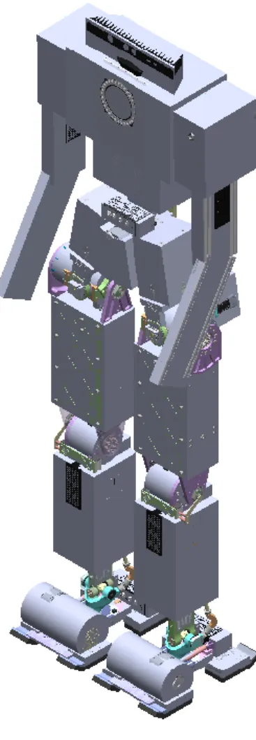
TigerBot comes from RIT’s multi-disciplinary senior design class. The original goal for TigerBot was to develop a robotic tour guide for RIT that would give tours to prospective students and other visitors and demonstrate engineering aspects and execution by example. With that idea in mind, the desired aspects and capabilities included being human-sized and proportioned, untethered, able to carry a quarter of its weight, 22 DOF including arms and head motion, able to walk, turn, recover from disturbances, and avoid obstacles, and have voice commands. Not all points were met, but the current robot acts as a platform for additional work and testing. TigerBot’s CAD design and physical build can be seen in Figure 2.

(a) (b)

This version of TigerBot was made by the 7th _{iteration of the senior design team. The project} started with small scale humanoids and scaled up to full size. The latest team was given the 6th iteration of TigerBot, which was the lower half of a full scale humanoid, from the waist down. The team deemed it inadequate, however, and designed TigerBot 7 from the ground up, using the motors from TigerBot 6.

3.2 TigerBot Anatomy

The anatomy of TigerBot follows a typical humanoid robot, as seen in Figure 3. Figure 3 also shows the conventional coordinate system. In addition to having the x-axis forward, y-axis to the side, and z-axis up, whenever ‘left’ or ‘right’ is mentioned, it refers to the robot’s left and right. Table 1 also specifies TigerBot’s height and other characteristics.

Table 1: Characteristics of TigerBot including height, width, and mass. Height (m) Leg length (m) Thigh Length (m) Shank Length (m) 1.689 0.9798 0.44288 4.3513 Foot Length (m) Foot Width (m) Stance Width (m) Mass (kg) 0.33921 0.20495 0.26154 51.51071

TigerBot’s legs features three-axis hip joints to resemble a ball joint, knee joints, two-axis ankles for roll and pitch of the feet, and an active toe and passive heel to allow for more natural walking gaits with actuation in the foot. The ankles are controlled through two linear actuators that connect to the back of the ankle. To control the ankle’s pitch, the actuators have to move at the same speed in the same direction, while to control the roll they have to move in opposite directions. In that way the ankle’s two DOF are controlled simultaneously by differing the linear actuators’ speed and direction. The exact velocities of the actuators come from taking the speeds to travel one degree per second for each axis, converting them to the speeds to move the desired change in angle in the desired time, and adding the two speeds for each actuator together to get velocities to move in both axes simultaneously. The knee has a belt-and-pulley system attached to a harmonic drive. The feet consist of an active toe and a passive heel. The toe is powered with a motor and harmonic drive, while the heel is passively dampened to help absorb shock while walking. Both the toe and the heel are connected to a central block connected to the yoke of the ankle. The soles of the feel have foam cushioning to help absorb shock while walking and load cells in the four segments, two as the toe and two as the heel. Figure 4 shows the ankle and foot.

Figure 4: The right shank and foot. This shows how the Teknic Clearpath servo connects to a linear actuator, which itself is attached to the back of the ankle.

TigerBot uses Teknic Clearpath servos which has multiple settings and control schemes available. The motors are set to the Step and Direction mode, so they can be used as stepper motors. The inputs to the motor include an enable, a direction input, and a step input; all three are digital inputs and the last takes pulse inputs. The motors also have a setting called Regressive Auto Spline (RAS), which is a time setting for automatic acceleration/deceleration on the scale of milliseconds.

The RAS time is kept low but is not completely turned off since it helps smooth the motion without having to have it programmed in externally. The motors are paired up with harmonic drives to increase the maximum torque with a 1:100 gear ratio except for the ankle joints. Absolute encoders are placed at the output of the harmonic drives for most of the joints. For the ankles, the absolute encoder is placed on the joint axis itself. For the rotational hip joints, an inductive absolute encoder is used. The servos have internal encoders, but they are only used for other modes of control and cannot be accessed directly by the user. Also, the output is modulated through the harmonic drive, so external encoders end up necessary.

The model for TigerBot includes 2 DOF arms that have been designed but not yet machined and installed on the real robot. The joints are shoulder flexion and abduction joints. There is no end-effectors designed, but the 2 DOF arms leaves it possible to mount some later; as they are, the arms could be controlled to keep balance while walking.

3.3 TigerBot Electronics and Software

For motor and sensor control, TigerBot uses an ODroid XU4 single-board computer as a central control unit and houses it in the chest with a cooling fan. A single-board computer is used because it can be installed within the robot itself and the robot would not require communicating to an external computer for basic control. The ODroid XU4 was chosen for its power compared to other single-board computers. The ODroid has the Ubuntu 14.04 Linux environment. This version of Ubuntu was used because it is compatible with ROS Indigo. ROS stands for Robot Operating System; it is a software infrastructure for robotics. It allows different components of a robot to communicate with each other using a node-topic structure. Nodes are executables that publish or subscribe to topics, which are lines of communication, though they do not know which node publishes messages or are subscribed to the topics. ROS uses software packages to

interface with different devices. For controlling TigerBot, the rosserial package is mainly used. This ROS package allows USB serial devices to act as nodes. ROS has multiple software versions, the latest being ROS Lunar. ROS Indigo was chosen for stability and the author’s familiarity with it; at the start of the project, ROS Kinetic was recently released but did not have a lot of packages compatible with it. ROS Lunar is out now as well but is still relatively new.

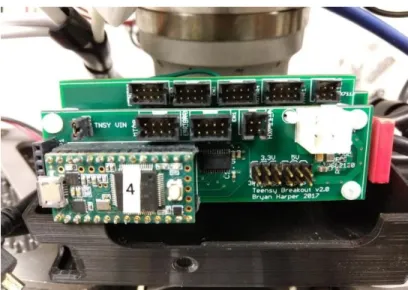
Each sublimb of the robot, e.g. the thigh and the shank, has a three-layer PCB stack that houses a Teensy microcontroller, which connects with up to three motors at a time. These PCB stacks, besides having chips and ports to connect the microcontroller to the motors and encoders, also have current sensors for the motor power lines, as the 75V DC power lines run through the PCB stacks. The layout of the PCB stack is the top layer for the Teensy, the middle layer for motor and encoder control, and the bottom later for power. The PCB stacks are in the thighs, shanks, pelvis, and chest. The thigh stack controls the hip abduction and flex and the knee, the shank stack controls the ankle and the toe, the pelvis stack controls the hip rotations and the waist abduction, and the chest stack is meant for the waist rotation. Figure 5 shows the PCB stack.

The microcontrollers plug into the single-board computer through external USB hubs and communicate through ROS. The microcontroller handles position-control of the joints using the encoder readings, which are received through the Serial Peripheral Interface (SPI). While reading the encoders, the microcontroller can run the stepper motor to the desired position, which comes from the single-board computer. The microcontroller will also send the encoder readings to the single-board computer.

The Teensys connects to ROS using the rosserial package. With the package, each Teensy initializes a separate node connected to the ROS master running on the single-board computer. The Teensy nodes can then load parameters for movements and subscribe and publish to topics. The single-board computer starts and ends the walking gaits by sending a message out to all the Teensys to act on. This is shown in Figure 6.

Figure 6: The flowchart of the connections between the ODroid, the Teensys, the encoders, and the motors. The ODroid sends commands and information to the Teensys to translate into commands for the motors. Each Teensy reads the encoders and sets the readings, the motors speeds, and the Teensy’s status to the ODroid.

TigerBot has a variety of sensors. As mentioned previously, there are current sensors for each motor and absolute encoders for each joint and DOF. There is also an IMU in the chest, and force sensors in the sole of each foot. The current sensors’ values can be used to calculate torque on the motors, which allows for a torque-controller, and for torque constraints. The absolute encoders are necessary for position-based control which is the type of control mainly used for this project.

TigerBot uses two varieties of absolute encoders. The kind mainly used is the AMT203 modular absolute encoder from CUI Inc. It has a resolution of 12 bits and communicates through SPI. It is used on the hip flex and abduction joints, the knees, and the ankle flex and abduction joints. The hip rotation joints cannot be measured with the AMT203 encoders since they need to be mounted between a stationary surface and a rotating shaft; the hip rotation joint is not conducive for such placement. Instead, IncOders from Zettlex are used. They are inductive angle encoders that consist of two rings that are meant to be mounted parallel but not touching each other. The difference in rotation between the two are measured through induction. This encoder also communicates with SPI, though it does not follow some aspects of SPI; for example, it does not have a slave select line as SPI usually expects.

Each encoder communicates to a Teensy, which publishes the encoder readings over a ROS topic. The encoders are connected to multiplexers, though the multiplexers are relevant mainly for the IncOders to separate their outputs, since they do not have a slave select and will output readings endlessly when powered. The PCB stacks can support up to three encoders, to correspond to the three possible motors it would control.

The IMU is from Variense, and has 3-axis gyroscopes, accelerometers, and magnetometers. It is a complete package that can plug into the single board computer through USB, so it does not require a Teensy like the other sensors for interpretation. It registers as a serial device and send its readings

continuously. Its outputs include readings from the accelerometer, gyroscopes, and magnetometers, and also the data as quaternions, Euler angles, and the heading. Each data type will have time stamps as well. The IMU can also take commands to change what data is streaming, change the resolution of the data, and test, calibrate, and check on different sensors. These readings could be used for monitoring the orientation of the chest and determine if the robot is tilting too far in one direction. To interpret and use these readings, the serial data will have to be parsed and then published on topics for the ROS nodes running the walking gaits to use. The pySerial library may be used for this.

Force sensors on the feet show how the robot’s weight is distributed, and if the feet are contacting the ground. TigerBot has a Six-Axis Force/Torque (SAFT) sensor module in each foot for precise force and torque feedback. This consists of a block placed within the foot beneath the ankle, containing strain gauges, Wheatstone half-bridges to amplify the readings, and analog-to-digital converters for translating the readings. The converters also connect to the load cells built into the foot. The single-board computer would connect to the SAFT block through a Teensy built into the SAFT block that takes readings and can be made into a ROS node like the other Teensys on TigerBot. Most of these sensor readings are not theoretically required to implement a walking gait, but they can be taken within simulation, so appropriate ranges for these values can be considered as well.

TigerBot is currently tethered, as the 75V DC power supply for the Teknic motors requires AC power. There are also 12V rails for each PCB stack, which gets converted locally to 5V for sensors, and 5V rails for the ODroid XU4 and the USB hubs. The Teensys can be powered from the PCB stack or from the USB hub.

Chapter 4: TigerBot Simulation

4.1 Creating a URDF

A Unified Robot Description Format (URDF) file is used in simulation and other software to describe how a robot is made up in joints and links. It starts with a root link, and follows a tree structure, branching when necessary. Joints and links each have properties such as location relative to the parent frame, joint limits and dynamics, and link inertia, visualization, and collision shape. A URDF then can be expanded on to fit other file formats for other pieces of software or be used as is.

The URDF for TigerBot starts with the torso and goes down to the hips, where it branched into the legs. The joints include the torso abduction and rotation joints, the hip rotation, abduction, and flex joints for each leg, the knees, the ankles’ abduction and flex, and the toe joints. The links follow the same order. The root link is the world link for Gazebo; this creates a virtual fixed joint between the Gazebo world and the model. The purpose of the link is to hold the model upright in the air as it spawns in. After the model gets in its starting pose, the joint is modified, then removed to have the robot land on its feet and balance on its own.

The model was based off the SolidWorks model for TigerBot. It includes 2-DOF arms that have not yet been added to the real-life robot. The URDF was made using an add-on, the Solidworks-to-URDF exporter. The URDF has all the leg joints defined, but the arms are static and considered part of the torso, and one of the torso joints (the continuous torso rotation joint) was made fixed, to stop drift in the joint (which would be fixed with the latest PID change).

To export the model, some changes were made in Solidworks. The model was split into different assemblies to represent each link. Some components were hidden to reduce the visual complexity. Coordinate systems and axes were defined to represent joints. Solidworks’s global

coordinate system is different from ROS’s defined system. For ROS, the x-axis is the forward direction, y-axis is horizontal, and z-axis is up. When defining coordinate systems in Solidworks, the ROS convention should be followed, but the coordinate systems can also be changed manually in the URDF itself.

The URDF has both visual and collision properties for each link, where the visual model is what the link will look like, and the collision model will be the invisible but physical model underneath. For complex robots, the visual and collision models are usually separate. Simulators use the collision model to identify collisions, both between the robot’s own links and between the robot and other objects. Having the collision model resemble the visual model can be a waste of computing power. It is beneficial to have the collision model follow the general shape of the robot but be otherwise featureless. For example, for a robot with wheels, the visual model might have a fully-defined tire, while the collision model just uses a cylinder. For TigerBot, creating a collision model independent of the visual model required making a simplified Solidworks model consisting of blocks that followed the dimensions of the real model. This is then exported, and the resulting STL file models are edited manually into the final URDF. The collision model can be seen in Figure 7.

Figure 7: The TigerBot SolidWorks model with the collision model overlaying it. The collision model mostly consists of blocks outlining the original model with some exceptions like the ankle yokes.

A URDF could be made manually, but the exporter takes care of the complex properties, such as the frame transformations, the inertial properties, and the visual properties. The exporter took time to set up and figure out, however, and has bugs that lead to problems before and after generating a URDF. Using the exporter might be the cause of some problems in using the URDF, e.g. trying to generate an ik-fast package, which is a solver for inverse kinematics.

Besides the visual and collision properties of the URDF, there is also joint limit properties, which is the range of angles and the maximum effort and velocity a joint can handle, and the joint

dynamics properties, which include damping and friction. The range of angles have not been adjusted to account for collision because another piece of software, MoveIt!, has collision checking and avoidance. For joint dynamics, arbitrary nonzero values have been included to keep the robot from acting unrealistically.

4.2 MoveIt!

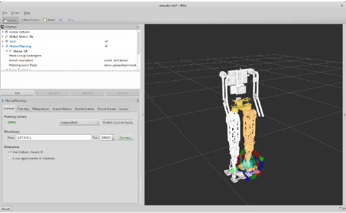
MoveIt! was set up for TigerBot as well. MoveIt! is software for robotic manipulation that handles path-planning, trajectory generation, kinematics, and more. It runs off ROS using a node to pull the robot’s description and characteristics from the parameter server, usually as a URDF, and provides services and topics to control a robot while also expecting certain topics for information on the robot’s current state. It requires a URDF and some set-up to generate a custom MoveIt! package for a robot. MoveIt! will generate a Semantic Robot Description Format (SRDF) file in combination with the URDF that describes planning groups, end-effectors, additional collision checking and transform information, and other properties. The planning groups which joints will be controlled while the others are left stationary, so the planning groups for TigerBot are the left leg and the right leg, from the hips to the foot, not including the toe joints. MoveIt! uses RViz to visualize the model. RViz is a 3D visualizer for ROS. Typically it is used for visualizing sensor data such as cameras and point clouds, but MoveIt! uses it for visualizing the robot’s pose and the movements it would make. It also uses a plugin in RViz to allow controlling the robot through clicking and dragging interactive markers on the end-effector of the robot. Figure 8 shows how the model appears in RViz.

Figure 8: TigerBot as seen in RViz when using TigerBot’s MoveIt! demo. TigerBot’s legs can be controlled and moved directly from RViz using the MoveIt! plugin.

MoveIt! could be used for controlling TigerBot, but it was used primarily for calculating inverse kinematics to control the feet. It used the Trac-IK Kinematics Solver plugin, since the default solver would not work properly in ROS Indigo for TigerBot. MoveIt! performs collision checking, so even without precise joint angle limits in the URDF, the inverse kinematics will take appropriate joint angles into account. The model’s origin, which is at the pelvis, is set at the world’s origin, so calculations are basically respective to the pelvis. The cartesian coordinates inputs for the inverse kinematics are distances from the hips to the feet, only in the x and y axes since the z-axis coordinate, the height, of the COM is inputted once and held constant. The joint values from the inverse kinetics can then be used in the simulation for walking.

4.3 Gazebo

4.3.1 Gazebo Overview

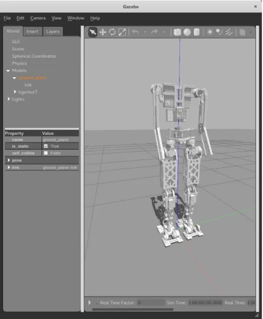
Gazebo is a 3D dynamic simulator designed to simulate robots which was chosen for its compatibility with ROS. Gazebo is different from RViz where RViz is kinematics based and Gazebo is physics-based. When using Gazebo, a world environment contains the robot and other models. The world can be set up to simulate the robot in different environments such as inside a room with furniture. The version is 7.0, which was upgraded from the default 2.0 version for ROS Indigo. Gazebo uses the Simulation Description Format, which is a format for describing the various elements and components of a robot. It can describe world-level characteristics down to robot-level and is designed to make up for some of URDF’s shortcomings. Gazebo can also use a URDF with the required SDF elements inserted. The additional Gazebo elements refer to how joints are controlled, and how the simulator should act relative to different joints and links. The additional Gazebo elements included in the URDF file for TigerBot include transmission element, which describe how each joint is controlled, dampening and stiffness, to keep the robot from moving unrealistically, and friction constants for the feet, since the foam on the soles of the feet are coated in rubber to reduce slipping. Figure 9 shows the TigerBot model in Gazebo.

The joints can be controlled by position, velocity, or effort, referring to what the joint uses to achieve its goal position. Position control is simply moving to the target position, velocity control is moving at specific speeds to the target, and effort is exerting a certain amount of force to move to the target. The position control setting is used in Gazebo. Due to a bug, the default position setting does not work in ROS Indigo, so position PID control is set instead. When Gazebo gets a desired position, instead of automatically moving to the position, Gazebo uses PID to determine the appropriate effort to apply to the joint to move to that position. The PID gains are set as ROS parameters, specific to each joint.

An issue caused by using position PID control was setting incorrect PID gains. Previously, the gains were off such that the joints were not reaching their desired positions; they would jerk towards the target angle but then settle at a lower value. This caused inaccurate trajectories and test results. The gains were changed through trial-and-error to settle quickly at the positions with no oscillation. The gains themselves are much higher than the previous values. The model will then hold positions and appear more rigid then before with incorrect gain values.

Figure 9: TigerBot as seen in Gazebo. The model spawns at the origin of the world. The simulation is currently paused, with the simulation time and the real time at zero.

Gazebo sets up a simulator clock to run off, which corresponds to the simulation world. When ROS keeps track of time, it will use the simulated time instead of real-time as a result. When talking about time in regards to simulation, it will refer to the simulated clock time.

4.3.2 Gazebo and ROS

Gazebo can stand alone or work with ROS. For integrating with ROS, Gazebo has a group of packages called gazebo_ros_pkgs. These allow control of the simulator, give access to data, and make Gazebo plugins for various sensors and such compatible with ROS. They also let URDFs be used alongside SDFs. To simulate robot control, Gazebo uses the ros_control package, which sets up controllers to handle groups of joints. Controllers in this context are interfaces that translates ROS commands into commands for the robot’s hardware. There are premade controllers that interface using ROS actions; they include effort, velocity, or position control and can take trajectory inputs or single inputs. The simulation for TigerBot uses a position controller to control the legs. The commands for the controller are sent to the controller through a command topic that takes an array of desired position values for each joint.

TigerBot currently has three joint position controllers: one for the hips and both legs, one for the torso rotation and abduction joints, and one for the toes. One the first controller is used for implementing the walking gaits, as the gaits currently do not actuate the torso and toes. Those joints are either held at a constant neutral position or are disabled through the URDF to simplify control.

The COM is important in generating a walking gait, so it is important to know its location and velocity. Gazebo publishes messages on topics detailing the model’s state and each of the links’ states. The messages detail the object’s pose, which is position and orientation, and the object’s twist, which is linear and angular velocity. By default, this is all in the world’s frame. The URDF

information is also accessible, as it gets loaded in as a ROS parameter for Gazebo to use. The URDF contains the mass of each link; this, in addition to the position and velocity of each link from the link state messages, means that the COM position and velocity can be calculated within the simulation. The feet positions are given in the link state messages as well, so the COM position can be compared to the feet positions for a general idea if the COM is within the support polygon. The x and y coordinates of the COM are represented with a sphere in Gazebo at a height of TigerBot’s ankles for a visual representation of the projection of the COM compared to TigerBot’s feet.

TigerBot’s COM is located between its thighs. To simplify calculations, it can be assumed to be at its pelvis instead, so when the COM’s position and velocity is required, the pelvis’s position and velocity are used instead.

TigerBot is spawned into Gazebo with a world link that fixes the model to a point in the air. To start TigerBot out in an initial pose, it is easiest to move to that pose in the air, then setting the robot on the ground to continue standing or start to walk. To simulate that behavior, the joint between the world link and the torso can be modified from a fixed joint to a prismatic joint in the z direction, letting the model slide down to the ground while still held upright, then removing the joint completely, so the model balances on its own.

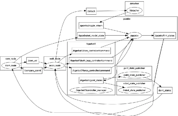
Figure 10 shows the layout of how the simulation works in ROS. The Gazebo node publishes the state of links in models, which is subscribed on by the COM node, which pulls information concerning the COM and the feet. These topics are subscribed to by the node running the walking gait, which also publishes commands to control TigerBot in Gazebo. These include commands to detach the model from the world link in Gazebo, which suspends the model in the air.

Figure 10: The plot of the topics and nodes in ROS for running the walking gait simulation.

4.4 Running the Walking Gait

4.4.1 Standing

Standing upright involves TigerBot with bent knees, feet spread, and a proportional-integral (PI) controller on the ankles’ pitch. TigerBot’s slight crouch serves to lower TigerBot’s COM for increased stability and make longer strides possible since the legs have more margin to stretch. The PI controller moves the ankle flex joint up or down to stop the robot from falling forward or back respectively. It uses the COM’s velocity for the error, since if the COM is too far forward or back, the robot would then start falling forward or back and have a nonzero velocity. When the COM has a velocity at zero, the robot is balanced. The integral part of the controller is necessary to keep the robot upright, but a derivative part is optional and is not included. The derivative part can be detrimental and cause jittering and instability.

The PI controller is for balance along the x-axis, and no controller is necessary along the y-axis. Previously an ankle roll controller was used in the same manner as the ankle pitch controller except using the COM velocity’s y component, which was then switched to a controller using the hips’ abduction joints. The second controller was used because resisting falling to the side using the hips is more natural and also more effective than using the ankles. However, modulating the hip abduction joints would cause greater discrepancy to the cartesian coordinates used to calculate the inverse kinematics compared to using the ankle roll joint. After correcting Gazebo’s PID changes, the robot did not need a controller to resist falling sideways, since the robot was rigid enough to balance. The controller for y-axis balance could still be used perhaps to control sideways velocity better.

4.4.2 Walking Gait Generation

4.4.2.1 Walking Gait using the LIPM

In the beginning, the plan was to follow the LIPM method of walking gait generation. This followed the equations shown in the literature survey and appeared as in Figure 11. The initial setup would start with the standing pose, the COM would shift over to the right foot, then the robot would take three steps and end with its feet together again. The equations output COM trajectories for each walking primitive, which were converted to distances between the COM and each foot by comparing the trajectories to the step coordinates. These distances were brought into MoveIt! to generate joint trajectories.

Figure 11: The graph of the COM trajectory generated by following the LIPM concept. The different colors of the trajectory indicate separate walk primitives. The feet of each step are outlined in matching colors to indicate the stance foot per primitive. The circle markers indicated the desired ZMP of each step, while the x markers indicate the actual ZMP calculated to fit the trajectory. Parameters include a step width of 0.3m, length of 0.1m, COM height of 1.07867m, a=15, and b=1.

Initially, instead of using inverse kinematics, MoveIt!’s path-planning functions were used. MoveIt! can take cartesian waypoints, generate a cartesian path, then calculate joint trajectories which included not only joint positions but also joint velocities, accelerations, effort, and timing. However, the timing did not follow the desired time width for each step, since the joint positions will be published at a constant rate, nor did it have consistent time increments between joint trajectory points. To normalize the timing, the times were scaled to fit the appropriate time range, and from plotting the joint trajectories, joint value points were extrapolated to match the desired consistent time increment.

Besides the walking primitives, MoveIt! was also used to generate trajectories for the swing foot as it took a step. The trajectory involved lifting the foot, moving it to the desired position, and placing it back at the original height. At the same time, the stance foot should naturally push backwards while following the COM trajectory during the step. Like the walking primitives, the

generated joint trajectories were scaled and extrapolated to match the necessary timing for a step to be completed.

The generated joint trajectories were loaded into ROS as parameters and were sent to the joint controllers periodically. The immediate problem was that the robot could not keep its balance while it leaned to the side and lifted the swing foot; it would fall sideways as it had too much momentum. It still needed some momentum to keep the robot balanced on the stance leg while taking a step, however. In an attempt to control the COM velocity, the theoretical values were taken from the calculated COM trajectories and were included in the same PI controllers used to keep balance while standing and now used to stay upright. The PI controllers controlled the ankle flex and ankle abduction and instead of a COM velocity setpoint of zero, the velocity setpoint would vary. This did not have much of an effect on its behavior.

When the PID gains were changed to make the robot more rigid, the execution of this gait changed. The robot would not immediately tip sideways but had a tendency to move backwards. This may come from the COM tending towards behind the robot, causing the robot to lean back more, and when the feet lifted, caused the robot to end up taking a step back.

The problem with using a gait generated from the LIPM method is likely that TigerBot does not match the single mass assumption. Instead of having most of the mass in the torso and negligible mass in the legs, TigerBot contains a significant amount of mass in its legs.

4.4.2.2 Walking Gait with ZMP Attempt

After being unsuccessful with the LIPM model method, a basic walking gait generation method was started from scratch; the gait would start with swaying to the side, then swaying with lifting the swing foot, then actually taking a step and looping the process. This process would keep the COM, used as an approximation for the ZMP, within the support polygon during the gait, since

the support polygon shrinks to consist the stance foot during the single support phase. The PI control to balance along the y-axis was also switched from the ankle abduction joint to the hip abduction joint at this point.

Leaning to the side uses the same COM positions for the initial sway calculated with the LIPM method. The movement of the swing feet came not from the MoveIt!-generated trajectories, but from adjusting the joints manually. The swing foot would have the starting position and the new position and would lift off the ground by moving the hip abduction, knee, and foot flex joints. The stance foot would also move back and down, to ‘kick’ against the ground. During the step, the PI controller for balance would be temporarily disabled for the swing foot, so the PI control of the ankle’s flex joint would not mess up the swing foot’s contact with the ground. Once the swing foot is down, the current position of the feet and COM was taken, and shifting the COM to the next stance foot was generated by plotting 20 points between the current COM position and the desired position and using MoveIt! to calculate inverse kinematics. These positions required manual joint adjustments as well. Then the new step would again be done using joint adjustments.

This method of generating IK values and manually adjusting joint values was largely ineffective and inconsistent. The robot would take unnatural looking poses to stay balanced, and the manual adjustments required trial-and-error. No more than three steps were scripted out, and they could not be looped to create a walking cycle. The gait was unlikely to be robust enough for the real robot to use.

As mentioned before, a significant error was having incorrect PID parameters for position control in Gazebo. This lead to joints not following the position commands. After changing the PID gains, the previous walking gait with manual joint adjustments was invalidated. However, the standing and walking execution became more consistent. Walking primitives were changed to not

be dependent on the location of the COM and the feet in the world frame, but rather just consist of the relative position of the feet to the hip.

4.4.2.3 Successful Walking Gait using the ZMP Concept

The current walking gait for TigerBot consists of moving the COM forward while keeping it within the support polygon. As mentioned previously, the COM is approximated to be at the hips, so solving inverse kinematics is from the hips to the feet. Also, the ZMP is assumed to be the projection of the COM on the ground plane. The walking gait used in simulation consists of both single and double support phases. The gait is shown in Figure 12, and its parameters in Table 2.

Figure 12: The graph of the walking gait used in simulation. Along with the COM trajectory, the feet are outlined in different colors per step to match each walking primitive’s stance foot

(expect the green indicates the starting pose) with the circle markers indicating the center of each foot.

Table 2: The parameters of the walking gait used in simulation.

Step Length (m) Step Width (m) COM (pelvis) height (m)

0.1 0.4 1.07867

The initial standing pose has the feet 0.4m apart, with a slight crouch to decrease the COM height by 0.06m. From the standing pose, the robot leans towards its right foot, so that the COM is above the foot. This makes the right leg the stance leg, and the left leg the swing leg. The left foot moves a step forward while the right foot shifts back. As the step happens, the robot is in the