.
Abstract—Large amount of software for embedded digital signal processing systems is written in assembly language. Software pipelining of loops is necessary to exploit the full potential of Very Long Instruction Word (VLIW) processors. For both understanding software pipelined loops and reverse compiling them to high level language code the software pipelined loops must be de-pipelined back to the original loops. In this paper we present technique for software de-pipelining of nested loops, demonstrate it with an example and evaluate the benefits of some software pipelined nested loops.
Keywords—software pipelining; de-pipelining; nested loops; DSP.
I. INTRODUCTION
EVERSE compilation techniques [4, 6, 13] have been applied to many areas such as porting legacy software written in assembly language to new architectures, link-time optimizers, and high-level debuggers [8]. Some key problems such as unpredication and unspeculation [20], reconstructing control structures [21], resolution of branch delays [2]-[3] and software de-pipelining [22]-[24] have been tackledrecently.
Software pipelining [14] is a loop parallelization technique used to speed up loop execution. It is widely implemented in optimizing compilers for very long instruction word (VLIW) and superscalar processors such as IA-64, Texas Instruments' C6X and StarCore’s SC140 DSP that support instruction level parallelism. Because nested loops take a large portion of execution time in scientific programs and DSP applications, software pipelining of nested loops have been extensively investigated [10, 15, 16, 17, and 18].
Software de-pipelining [22]-[23] is the reverse of software pipelining. This technique involving only single loops has been incorporated into a reverse compiler for the Texas Instruments C6X architecture [2]. We extend this technique to handle nested loops in digital signal processing (DSP) applications. This paper first presents a formal description of software pipelining and de-pipelining. We then analyze the existing software pipelining techniques and present our software de-pipelining technique for two-level nested loops. To illustrate the process, we present a working example. Finally, we provide our experimental results.
Nerina Bermudo and Andreas Krall are with Christian Doppler Laboratory Insitut für Computersprachen – Technische Universität Wien,Vienna, Austria
(email: {nerina, andi}@complang.tuwien.ac.at)
Bogong Su is with Dept. of Computer Science, William Paterson University, Wayne, NJ, USA (phone: 1-973-720-2973; fax: 1-973-720-2979; email: [email protected])
Jian Wang is with LTE Software Design, Ericsson Canada, Ottawa, Canada (email: [email protected])
II. FORMAL DESCRIPTION OF PIPELINING AND DE-PIPELINING OF TWO-LEVEL NESTED LOOPS
Data dependence is one of the major constraints for loop transformation such as software pipelining and de-pipelining. It is essential to understand how we represent data dependence of two-level nested loops.
Each iteration of a two-level nested loop is identified by its index vector(i1,i2), where i1 and i2 are the values of the outer and inner loop index, respectively. Thus, an instance of an operation op in a two-level nested loop is represented as(op,(i1,i2)). For any two instances, (op1,(i1,i2)) and(op2,(j1, j2)), if there is a data dependence between them, then we say that there is a data dependence between op1 and
2
op with a distance vector of (d1, d2), where dk = ik – jk for k
= 1 or 2. Like a data dependence in a single-level loop, a delay
δ is associated with each data dependence in a nested loop. The data dependence graph (DDG) of a two-level nested loop, therefore, is represented as (O, E,(d1, d2), δ), where O is
the node (operation) set, E is the (data dependence) edge set,
(d1, d2) and δ are the distance vector and the delay,
respectively, on each data dependence edge. Although delay δ is associated with an edge in the DDG, it is actually the execution time of the source operation op, we sometimes also use δ(op); δ(op) and δ(e) can be exchangeable used when op is the source operation of dependence edge e. However, DDGs with distance vectors are inconvenient in use during software pipelining or loop de-pipelining. We proposed linearized DDGs to represent data dependences of the two-level nested loops.
Definition 1 Given a two-level nested loop and its DDG, G
= (O, E,(d1, d2), δ), the linearized DDG of G is defined as
LG = (O, E, ld, δ), where, for each edge e, ld(e) = n2*d1(e)+
d2(e), and where n2 is the trip count of the inner loop;
Using the concept of linearized DDG, an instance of an operation op in a nested loop, (op,(i1,i2)), can be also represented as (op, li), where li = n2*i1 + i2. liis called the
linearized index of the index vector (i1, i2). It is a one to one
mapping between an index vector and its corresponding
linearized index.
Now we are ready to present the formal description of loop schedule, software pipelining and de-pipelining for two-level nested loops.
Definition 2 Given a two-level nested loop and its DDG, G
= (O, E,(d1, d2), δ), generate G's linearized DDG, LG = (O, E,
ld, δ). We define loop schedule σ as a mapping function from
O x N to N where N is a nonnegative integer set. σ(op,li) denotes the cycle number in which the instance of operation op
with the linearized index li is issued for execution. Note that σ
Software De-Pipelining for Nested Loops
Nerina Bermudo, Andreas Krall, Bogong Su, and. Jian Wang
is a valid loop schedule if and only if the following three conditions are satisfied:
(1) resource constraint: in any cycle, there must be no hardware resource conflict;
(2) data dependence constraint: for any data dependence edge e = (op1,op2) and for any linearized index j,
σ(op1, j) + δ(e) ≤ σ(op2 , j + ld(e));
(3) cyclicity constraint: σ must be expressible in the form of
a loop, that is, there must be an integer II, for any operation
op in the nested loop and for any linearized index j>1,
σ(op, j) = σ(op, j-1) + II*(j-1),II is called the
linearized initiation interval.
Definition 3 Software pipelining of a nested loop is to find a valid loop schedule with minimum linearized initiation interval.
Definition 4 Given a nested loop and its DDG,
G = (O, E,(d1, d2), δ), generate G's linearized DDG,LG =
(O, E, ld, δ). De-pipelining is to find a valid loop schedule σ which satisfies the following two conditions:
(1) for any operation op and for any linearized index j,
σ(op, j) + δ(op) ≤ σ(op, j +1);
(2) for any two operationsop1 and op2, and for any
linearized index j, σ(op1, j) + δ(op1) ≤ σ(op2 , j +1); Definition 5 VLIW Instruction VIi = {opi1, opi2, …, opin | all n instructions can be executed at the same CPU clocki without any resource conflict }
The goal of software pipelining is to speed up the execution time of a nested loop. To do so, software pipelining overlaps operations from different iterations to exploit instruction level parallelism. De-pipelining, however, is to execute the loop sequentially, i.e., one iteration after another. Thus, in a de-pipelined loop, operations from different iterations will not be overlapped and the loop-carried dependence is automatically satisfied.
Different approaches have been proposed to software pipeline a two-level nested loop. It is important that we should first check if a two-level nested loop is software pipelined. The idea behind our method is to verify the loop-carried data dependences in the linearized DDG. If the dependences are broken, the nested loop is likely to be software pipelined.
III. EXISTING NESTED LOOP SOFTWARE PIPELINING APPROACHES
So far all software pipelining techniques of nested loops are for two level nested loops only. Most are applied to VLIW architectures such as the Itanium and TIC6x DSP. They have some common characteristics shown below.
The inner loop is software pipelined first for a better chance of overlapping with instructions of the outer loop. Unrolling or Unroll-and-Jam [5] of the inner loop is necessary before software pipelining the outer loop [7, 19].
Outer loop software pipelining overlaps outer loop iterations including the epilog and prolog of the inner loop with each successive iterations of the outer loop [10, 15]. Performing outer loop software pipelining often requires the use of large
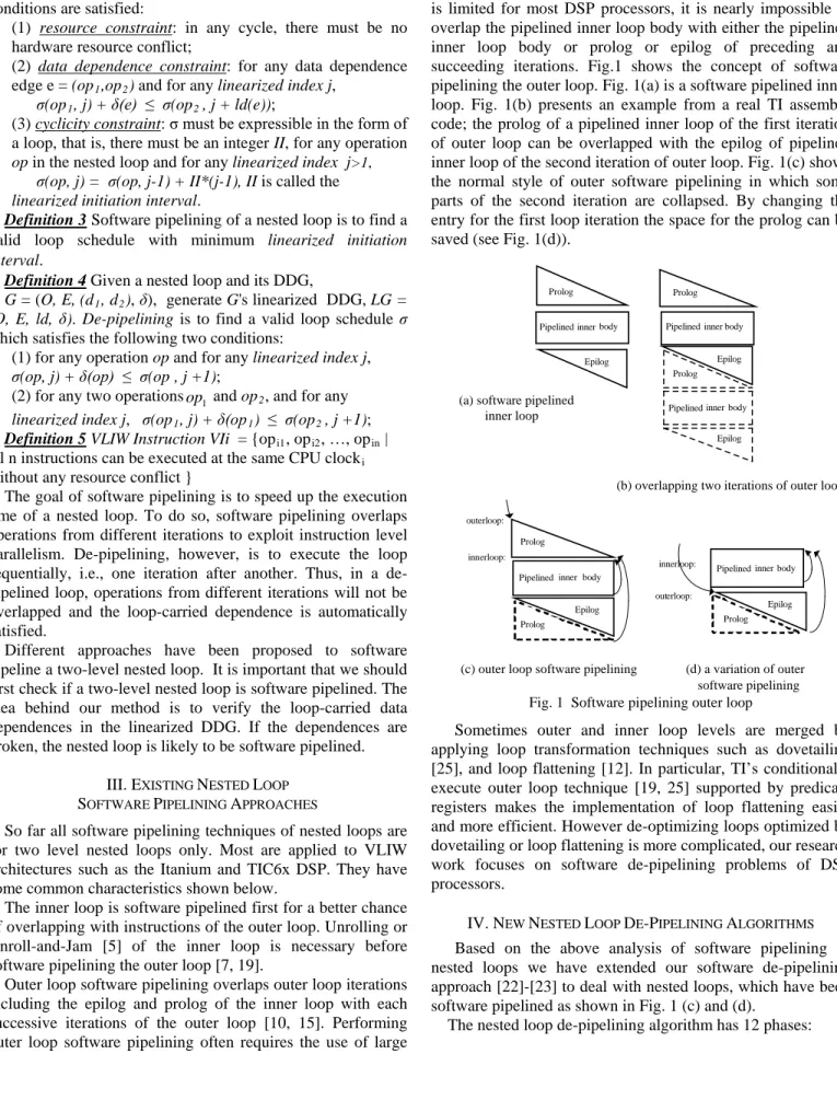
number of registers. Because the number of available registers is limited for most DSP processors, it is nearly impossible to overlap the pipelined inner loop body with either the pipelined inner loop body or prolog or epilog of preceding and succeeding iterations. Fig.1 shows the concept of software pipelining the outer loop. Fig. 1(a) is a software pipelined inner loop. Fig. 1(b) presents an example from a real TI assembly code; the prolog of a pipelined inner loop of the first iteration of outer loop can be overlapped with the epilog of pipelined inner loop of the second iteration of outer loop. Fig. 1(c) shows the normal style of outer software pipelining in which some parts of the second iteration are collapsed. By changing the entry for the first loop iteration the space for the prolog can be saved (see Fig. 1(d)).
Prolog
Epilog
Pipelined inner body Pipelined inner body Pipelined inner body
Prolog
Prolog Epilog
Epilog
(b) overlapping two iterations of outer loop
innerloop: outerloop:
Pipelined inner body
Prolog Prolog
Epilog
Pipelined inner body innerloop:
outerloop:
Prolog Epilog
(c) outer loop software pipelining (d) a variation of outer software pipelining
Fig. 1 Software pipelining outer loop
Sometimes outer and inner loop levels are merged by applying loop transformation techniques such as dovetailing [25], and loop flattening [12]. In particular, TI’s conditionally execute outer loop technique [19, 25] supported by predicate registers makes the implementation of loop flattening easier and more efficient. However de-optimizing loops optimized by dovetailing or loop flattening is more complicated, our research work focuses on software de-pipelining problems of DSP processors.
IV. NEW NESTED LOOP DE-PIPELINING ALGORITHMS Based on the above analysis of software pipelining of nested loops we have extended our software de-pipelining approach [22]-[23] to deal with nested loops, which have been software pipelined as shown in Fig. 1 (c) and (d).
The nested loop de-pipelining algorithm has 12 phases: (a) software pipelined
1.Control flow graph CFG reconstruction and natural loop analysis: Use natural loop analysis [1] from the given segment of assembly code to find CFG, the entries of outer loop and inner loop, the inner loop body and the end of outer loop.
2.Software-pipelined loop checking: For each instruction pair (opi, opj) in inner loop body, if opi data precedes opj and the latency of opi ≥ the distance between opi and opj, then the inner loop is software pipelined. Similarly, we can check whether the outer loop is software pipelined.
3. Identification of the pre-area and post-area of the outer loop: Pre-area contains the instructions before the inner loop body, which includes the prolog of the software-pipelined inner loop and the initialization parts of inner loop and outer loop.
Post-area contains the instructions following the inner loop body which includes the epilog of the software-pipelined inner loop; it may also include the duplicated instructions of prolog of the software-pipelined inner loop. 4.Transformation of the space saving variation of outer
software pipelining: If the given software pipelined code is a space saving variation as shown in Fig. 1(d), it must be transformed to the normal style as shown in Fig. 1(c) first. 5.De-pipelining the outer loop: If the outer loop is software-pipelined normally, remove those instructions in post-area which are the copies of instructions in pre-area and adjust the entry of outer loop to form the prolog of inner loop. 6.Live variable analysis: Search all last_instructions in the
inner loop, which contains all memory store instructions and register-written instructions if those written registers are live variables after inner loop exit
7.Identification of the prolog and epilog: Starting from the inner loop entry search upward to all VLIW instructions containing instructions that exist in inner loop body, the highest VLIW instruction is the upper boundary of the prolog. The lower boundary of the epilog is obtained in a similar manner.
8.Prolog and Epilog recovery: If the prolog is collapsed, unroll the inner loop body and check every instruction in the unrolled copy; if it does not modify any part of the machine state, then it is the collapsed instruction. Epilog can be recovered in a similar manner.
9.Build LBDDG: In prolog and inner loop body, build a data dependency graph called LBDDG.
10.Scheduling: From last_instructions using list scheduling, arrange the partial order list of the critical path of LBDDG in a bottom-up manner to get a sequential code, and then insert the rest instructions in the non-critical path; finally obtain a sequentialized code which is semantically equivalent to the original software pipelined inner loop. 11.Inner loop replacement: Replace the software-pipelined
inner loop by its sequentialized code.
12.Outer loop scheduling: Build the data dependency graph for all VLIW instructions beyond and after the sequentialized inner loop respectively; then use list
scheduling to form the sequential code beyond and after the sequentialized inner loop to form the final sequential code.
Reference [24] presents the detail algorithms of each phase. V. WORKING EXAMPLE
We have taken an assembly language version of a FIR function as a working example to demonstrate our de-pipelining technique on two-level nested loops. The unrolled inner loop is shown in Fig. 2(a). The machine architecture is similar to TIC62. However, for simplicity, we assume that all branch, load, and multiplication instruction have only one delay slot (latency is two clock cycles) and other instructions have no delay slots. Fig. 2(b) shows its optimized assembly code, the symbol “||” in front of an instruction indicates that the instruction is executed in parallel with the one immediately above it. All instructions executed in parallel belong to a single VLIW instruction.
Fig. 2(c) is a new form for assembly code to explicitly express the instructions that are executed in parallel, where each row is a VLIW instruction. By using natural loop analysis [1] we can find that this is a two level nested loop; where outloop and loop are the entries of the outer loop and inner loop respectively.
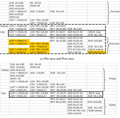
The length of the inner body is two because the latency of branch instruction is two. By using the software-pipelined loop checking, we find out that the inner loop has been software-pipelined, because the LDH *++A5(4),A9 and MPY A7,A9,A7 are located in the first VLIW instruction of inner loop but the LDH instruction writes register A9 which is read by MPY instruction and LDH’s latency is two cycles. Fig. 2(c) also shows the pre-area and post-area. Some instructions in pre-area have copies (as shown with shadow) in post-area; this working example is the type as Fig.1(c) shown. Similarly, by using the Software-pipelined loop checking, we find out that the outer loop has also been software-pipelined. Because in the post_area, the LDH *++B6(4),A7 instruction writes register A7 which is read by MPY A7,A9,A7, but the MPY instruction is located earlier than the LDH instruction even LDH’s latency is two cycles.
Fig. 2(d) is the result of De-pipelined outer loop. The duplicated instructions in post-area have been removed. Fig. 2(d) also shows the prolog and epilog parts of software-pipelined inner loop found in the Identification of the prolog and epilog phase. In this simple example both prolog and epilog are not collapsed. By using live variable analysis we find that ADD A0, B5, A0 is the last_instruction. Fig. 2(e) shows the LBDDG of the inner loop which is the result of the Build_LBDDG phase. In Fig. 2(f) the inner loop is replaced by a sequential loop which is semantically equivalent to the software-pipelined loop from the Inner loop replacement phase. Fig. 2(g) presents the final sequential code produced from the Outer loop scheduling phase.
void fir (short x[], short h[], short y[]) {
for (j=0; j<50; j=j+2) { sum=0; x0=s[j];
for (i=0; i<64; i+=2) { x1=x[j+i+1]; h0=h[i]; sum+=x0*h0; x0=x[j+i+2]; h1=h[i+1]; sum+=x1*h1; } y[j]=sum; } }
short i, j; int sum; short x0, x1, h0, h1;
(a) FIR C source code
(c) Pre-area and Post-area
(d) After de-pipelining outer loop
(e) Building LBDDG of innerloop
(b) FIR assembly code (f) After replacing inner loop (g) Final sequential assembly code
Fig. 2 Working example
SUB A4,4,B6 MV B4,A3
MVK 0x19,B1 ZERO A8
ADD A8,A4,A0
LDH *++B6(4),A7 ADD 2,A0,B4 SUB A3,4,A5 Pre-area
MVK 0x20,B0 ZERO A0
LDH *++A5(4),A9 LDH *B4++(4),B5
LDH *+A5(2),A3 SUB B0,1,B0
outloop LDH *++A5(4),A9 LDH *B4++(4),B5 MPY A7,A9,A7
LDH *+A5(2),A3 LDH *+B4(2),A7 MPY B5,A3,B5 SUB B0,1,B0
loop LDH *++A5(4),A9 LDH *B4++(4),B5 MPY A7,A9,A7 ADD A0,A7,A0 [ B0] B loop
LDH *+A5(2),A3 LDH *+B4(2),A7 MPY B5,A3,B5 ADD A0,B5,A0 SUB B0,1,B0
MPY A7,A9,A7 ADD A0,A7,A0
LDH *++B6(4),A7 MPY B5,A3,B5 ADD A0,B5,A0 MVK 0x20,B0
LDH *++A5(4),A9 LDH *B4++(4),B5 ADD A0,A7,A0 Post-area
LDH *+A5(2),A3 ADD A0,B5,A0 SUB B1,1,B1
LDH *++A5(4),A9 LDH *B4++(4),B5 STH A0,*A6++(4) [ B1] B outloop
LDH *+A5(2),A3 LDH *+B4(2),A7 ADD 4,A8,A8 ADD A8,A4,A0
SUB A4,4,B6 || MV B4,A3 MVK 0x19,B1 || ZERO A8 ADD A8,A4,A0 LDH *++B6(4),A7 || ADD 2,A0,B4 || SUB A3,4,A5 MVK 0x20,B0 ZERO A0 LDH *++A5(4),A9 || LDH *B4++(4),B5 LDH *+A5(2),A3 || SUB B0,1,B0 LDH *++A5(4),A9 || LDH *B4++(4),B5 || MPY A7,A9,A7 LDH *+A5(2),A3 || LDH *+B4(2),A7 || MPY B5,A3,B5 || SUB B0,1,B0 LDH *++A5(4),A9 || LDH *B4++(4),B5 || MPY A7,A9,A7 || ADD A0,A7,A0 || [ B0] B loop LDH *+A5(2),A3 || LDH *+B4(2),A7 || MPY B5,A3,B5 || ADD A0,B5,A0 || SUB B0,1,B0 MPY A7,A9,A7 || ADD A0,A7,A0 LDH *++B6(4),A7 || MPY B5,A3,B5 || ADD A0,B5,A0 || MVK 0x20,B0 LDH *++A5(4),A9 || LDH *B4++(4),B5 || ADD A0,A7,A0 LDH *+A5(2),A3 || ADD A0,B5,A0 || SUB B0,1,B0 || SUB B1,1,B1 LDH *++A5(4),A9 || LDH *B4++(4),B5 || STH A0,*A6++(4) || ZERO A0 LDH *+A5(2),A3 || LDH *+B4(2),A7 || ADD 4,A8,A8 || ADD A8,A4,A0 || [ B1] B outloop ADD 2,A0,B4 || SUB A3,A4,A5
SUB A4,4,B6 MV B4,A3
MVK 0x19,B1 ZERO A8
outloop ADD A8,A4,A0
LDH *++B6(4),A7 ADD 2,A0,B4 SUB A3,4,A5
MVK 0x20,B0
ZERO A0 Prolog
LDH *++A5(4),A9 LDH *B4++(4),B5
LDH *+A5(2),A3 SUB B0,1,B0
LDH *++A5(4),A9 LDH *B4++(4),B5 MPY A7,A9,A7
LDH *+A5(2),A3 LDH *+B4(2),A7 MPY B5,A3,B5 SUB B0,1,B0
loop LDH *++A5(4),A9 LDH *B4++(4),B5 MPY A7,A9,A7 ADD A0,A7,A0 [ B0] B loop
LDH *+A5(2),A3 LDH *+B4(2),A7 MPY B5,A3,B5 ADD A0,B5,A0 SUB B0,1,B0
MPY A7,A9,A7 ADD A0,A7,A0
MPY B5,A3,B5 ADD A0,B5,A0 MVK 0x20,B0
ADD A0,A7,A0 Epilog
ADD A0,B5,A0 SUB B1,1,B1
STH A0,*A6++(4) [ B1]B outloop
ADD 4,A8,A8
SUB A4,4,B6 MV B4,A3
MVK 0x19,B1 ZERO A8
outloop ADD A8,A4,A0
LDH *++B6(4),A7 ADD 2,A0,B4 SUB A3,4,A5
MVK 0x20,B0 ZERO A0 loop LDH *++A5(4),A9 LDH *+A5(2),A3 LDH *B4++(4),B5 MPY A7,A9,A7 MPY B5,A3,B5 SUB B0,1,B0 LDH *+B4(2),A7 ADD A0,A7,A0 [ B0] B loop ADD A0,B5,A0 STH A0,*A6++(4) MVK 0x20,B0 SUB B1,1,B1 [ B1] B outloop ADD 4,A8,A8 SUB A4,4,B6 MV B4,A3 MVK 0x19,B1 ZERO A8 outloop ADD A8,A4,A0
LDH *++B6(4),A7 ADD 2,A0,B4 SUB A3,4,A5 MVK 0x20,B0 ZERO A0 loop LDH *++A5(4),A9 LDH *+A5(2),A3 LDH *B4++(4),B5 MPY A7,A9,A7 MPY B5,A3,B5 SUB B0,1,B0 LDH *+B4(2),A7 ADD A0,A7,A0 [ B0] B loop ADD A0,B5,A0 STH A0,*A6++(4) MVK 0x20,B0 SUB B1,1,B1 [ B1]B outloop ADD 4,A8,A8 LDH *++B6(4),A7 LDH *++B6(4),A7 LDH *B4++(4),B5 LDH *+A5(2),A3 SUB B0,1,B0
LDH *++A5(4),A9 LDH *B4++(4),B5 MPY A7,A9,A7
LDH *+A5(2),A3 LDH *+B4(2),A7 MPY B5,A3,B5 SUB B0,1,B0
LDH *++A5(4),A9 LDH*B4++(4),B5 MPY A7,A9,A7 ADD A0,A7,A0 [ B0] B loop
VI. EXPERIMENT
Several nested loops have been software de-pipelined using the algorithms described in this paper. The test programs are hand-written typical DSP applications. Table 1 presents the results of software de-pipelining the nested loops in these programs.
The first column contains the name of the function. FIR4 implements an FIR filter, Vitgsm is a GSM decoder, and the last two loops correspond to routines that perform VSELP vocoder codebook search. The second column provides information about the optimizations performed on the different loops which, apart from software pipelining, consist of loop unrolling the innermost loop several times.
The next column shows the loop counters for inner and outer loops (represented by in and out, respectively) in the C implementation of the different functions. The C code for the Codebook search routine was not accessible to us. The next two columns compare loop counter initial values and body lengths of both inner and outer loops before and after
de-pipelining. The length is computed based on VLIW instructions. Note that the VLIW instructions of the inner loop are included in the outer loop.
Since the software de-pipelining is intended to reduce the complexity of the code, total number of sequential instructions and branches are also compared before and after the de-pipelining. Here sequential instructions and not VLIW instructions are counted. After software pipelining the loop code is written in a sequential form. Therefore, the comparison in terms of sequential instructions is more representative than the comparison of number of VLIW instructions.
The number of branches also provides information on how much it is easier to understand the sequentialized code for the loops and the corresponding control flow graph. After de-pipelining all examples have only two branches, which involve the jump to the inner loop entry and the jump to the outer loop entry.
TABLE 1 EXPERIMENT RESULT
Function Name Optimization approaches
C code Assembly code De-pipelining result
Loop count Loop count length Instr.
number Branch number
Loop count length Instr.
number Branch number inner outer in out in out in out in out in out
Fir4 1. unrolling 4 times 2. software pipelining software pipelining to save prolog N M N/4 M/2 4 16 99 3 N/4 M/2 34 40 54 2 Vitgsm GSM rate-1/2 convolutional decoder 1. innermost unrolled. 2.software pipelining software pipelining 8 M 8 M 3 11 79 4 8 M 22 24 65 2 Codebook search (Loop 1) 1. software pipelining 2. unrolling software pipelining - - 18 M 2 8 59 6 21 M 12 25 39 2 Codebook search (Loop 2) 1. software pipelining 2. unrolling software pipelining - - 8 M 2 8 98 6 11 M 12 25 59 2 VII. RELATED WORK
Since Cifuences and her colleagues presented their work, many decompilation techniques have been published [4, 6, 8, 13, 26]. However, few papers tackle deoptimizaiton techniques, in particular, fewer still are decompilation papers that involve loops and instruction-level parallel architectures.
Snavely, Debray and Andrews [20] present instruction level deoptimization approaches on Intel Ianium including unpredication, unscheduoing and unspeculation. However they did not tackle loop optimization and software de-pipelining. Wang et al. [27] apply un-speculation technique on modulo scheduled loops to make the code easier to understand.
Stiff and Vahid [21] use loop rerolling technique for binary-level coprocessor generation, which is the reverse of loop unrolling - a popular loop optimization. However, they did not deal with software pipelining.
Zhang et al. [28] propose to use a propositional calculus technique to recover high level control constructs from binary executable code.
Modern DSP such as Texas Instruments’ TMS320C6000 has rather long branch delay slots and allows branches to issue in the delay slots of other branches resulting in high efficient but cryptic code. Cooper et al. Reference [9] presents a method to correctly build CFG for scheduled code in the presence of branches within delay slots. Bermudo and Krall [2]-[3] present an efficient algorithm to construct CFG having
no branch instructions with delay slots making the code be easy understandable and processed by a reverse compiler.
Su et al. present software de-pipelined technique [22]-[23] for single level loops. Their method based on building LBDDG in software pipelined loop can convert the complicated software pipelined loop code to a semantically equivalent sequential loop.
VIII. CONCLUSION
In this article we presented a method for software de-pipelining of nested loops. This method is an extension of an algorithm for single loops, which has been integrated in a reverse compiler for assembly language programs for digital signal processors. Our extended method has been evaluated by applying it to four software pipelined loops. We are able to recover a sequential representation of the pipelined loop.
We are working with loop de-optimization techniques focusing on those loops optimized by loop unrolling and software pipelining, which are popular in modern DSP compiler generated code.
ACKNOWLEDGMENT
This work was supported in part by the Christian DopplerForschungsgesellschaft and Infineon. Bogong Su was partly supported by the Center for Research, College of Science and Health, William Paterson University.
REFERENCES
[1] A. V. Aho, M. Lam, R. Sethi, and J. D. Ullman. Compilers: Principles, Techniques, and Tools.2nd ed. Addison-Wesley, 2007.
[2] N. Bermudo. Low-level reverse compilation techniques. PhD Thesis. Technische Universität Wien. October, 2005.
[3] N. Bermudo, Nigel Horspool and A. Krall, Control flow graph reconstruction for reverse compilation of assembly language programs with delayed instructions, Proc. of SCAM2005, 2005.
[4] G. Caprino, Decompiler Design, Backer Street Software, http://www.backerstreet.com/decompiler/decompilers.htm, 2009.
[5] S. Carr, C. Ding, and P. Sweany, Improving Software Pipelining with Unroll-and-Jam, Proc. of the Twenty-Ninth Annual Hawaii International Conference on System Sciences, 1996.
[6] G. Chen, at el., A Refined Decompiler to Generate C Code with High Readability, Proc. of the 17th Working Conference on Reverse Engineering, 2010.
[7] C. Chung and X. Fu, Achieving better code optimization in DSP designs, EETimes, June 27, 2005.
[8] C. Cifuentes, Reverse Compilation Techniques, Ph.D Dissertation, Queensland University of Technology, Dept. of CS, 1994. of 8th Working Conference on Reverse Engineering, 2001.
[9] K. D. Cooper, T. J. Harvey, and T. Waterman. Building a Control Flow Graph from Scheduled Assembly Code. TR02-399. Rice University, June 2002.
[10] M. Fellahi and A. Cohen, Software Pipelining in Nested Loops with Prolog-Epilog Merging, Lecture Notes in CS, SpingerLink, 2009. [11] J. Fisher, Trace Scheduling: A Technique for Global Microcode
Compaction, IEEE Tran. On Computers, Vol. c-30, NO. 7, July 1981. [12] A. Ghuloum and A. Fisher, Flattening and parallelizing irregular,
recurrent loop nests, Proc. Of 5th ACM SIGPLAN symposium on Principles and Practice of Parallel Programming, 1995.
[13] A. Johnstone, et al., Reverse Compilation of Digital Signal Processor Assembler Source to ANSI-C, Proc. of ICMS99, 1999.
[14] M. Lam, Software pipelining: An effective scheduling technique for VLIW machines, Proc. Of SIGPLAN 88 Conference on Programming Language Design and Implementation, 1988.
[15] K.Muthukumar and G. Doshi, Software pipelining of nested loops. In R. Wilhelm, editor, CC2001, LNCS 2027, pages 165-181. Springer-Verlag, Berlin Heidelberg, 2001.
[16] D. Petkov, Efficient pipelining of nested loops: Unroll-and-Squash, Master Thesis, MIT, 2001.
[17] J. Ramanujam, Optimal software pipelining of nested loops, Proc. of the 8th International Symposium on Parallel Processing, 1994.
[18] H. Rong, Z. Tang, R. Govindarajan, A. Douillet, G. Gao, Single-dimension software pipelining for multi-Single-dimensional loops, Proc. of the international Symposium on Coded Generation and Optimization, 2004. [19] R. Scales, Nested Loop Optimization on the TMS320C6x, Application
Report SPRA519, Digital Signal Processing Solutions February, Texas Instrument, 1999.
[20] N. Snavely and S. Debray, Unpredication, unscheduling, unspeculation: Reverse engineering Itanium executables, IEEE transactions on Software Engineering, 31(2), Feb., 2005.
[21] G. Stiff and F. Vahid, New Decompliation Techniques for Binary-level Co-processor Generation, Proc. of ICCAD-2005, pp. 547-554Nov. 2005. [22] B. Su, J. Wang, E. Hu, and J. Manzano, De-pipeline a Software
Pipelined Loop, Proc. of ICASSP 03, June 2003.
[23] B. Su, J. Wang, E. Hu, and J. Manzano, Software de-pipelining Technique, Proc. of SCAM2004, 2004.
[24] B. Su and J. Wang, Algorithms of Nested Loops De-pipelining, Tech. Report, Dept. of CS, WPU, 2012.
[25] TMS320C6000 Programmer’s Guide, SPRU198G, August 2002. [26] J. Wang and B. Su, Software pipelining of nested loops for real-time
DSP architectures, Proc. of ICASSP 98, May 1998.
[27] M. Wang, R. Zhao, J. Pang, and G. Cai, Un-speculation in Modulo Scheduled Loops, Proc. of 2nd Int. Multisymposium on Computer and Computational Sciences, pp. 486-489, 2008.
[28] J. Zhang, R. Zhao, J. Pang, and W. Fu, Decompiling High-level Control Structures with Propositions, Proc. of 3rd International Symposium on Intelligent Information Technology Application, 2009.