PhD Program in Bioinformatics
Integrated Analysis and Application Pipelines
for Complex Disease Data
Dissertation
zur Erlangung des Grades
Doktor der Naturwissenschaften
der Naturwissenschaftlich-Technischen Fakult¨
at III
Chemie, Pharmazie, Bio- und Werkstoffwissenschaften
der Universit¨
at des Saarlandes
von
Christian Spaniol
June 2015
Dekan:
Prof. Dr.-Ing Dirk Bähre Prüfungsausschuss:
Prof. Dr. Uli Müller (Vorsitzender)
Prof. Dr. Volkhard Helms (1. Berichterstatter)
Prof. Dr. med. Matthias Riemenschneider (2. Berichterstatter) Dr. Jessica Hoppstädter (Akad. Mitarbeiterin)
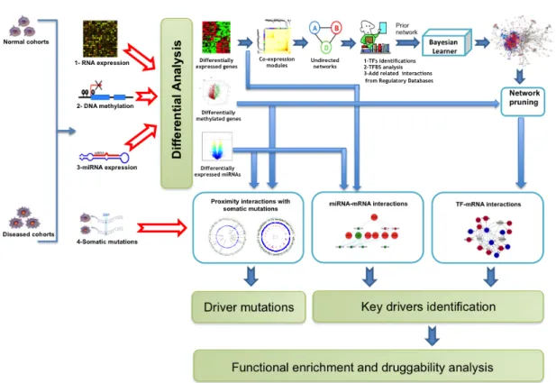
The increasing amount of biological data available from high-throughput technolo-gies poses great interdisciplinary challenges to research. Today, cost-efficient plat-forms generate manifold types of data and allow to build comprehensive resources that include but are not limited to genomics, proteomics, and metabolomics on a systemic scale. In order to adapt to this development in the post-wetlab analysis, computer scientists in computational biology work on methods and software frame-works that are able to account for data size and diversity, and allow to scrutinize data in respect to a specific context, such as the emergence of diseases.
Aiming for this, we first present a desktop software framework designed to integrate biological data that features a uniform interface to perform consecutive analysis steps managed by an automated task processing system. The extensibility of the platform based on a concise plugin interface was used for a study on breast cancer for which we developed a plugin to derive gene regulatory networks.
From this analysis, we derived a general approach to generate transcription factor-microRNA regulatory networks and built a webservice available for public use: TFmiR. Using differentially expressed sets of mRNAs and miRNAs, TFmiR generates a network with experimental or predicted evidence and provides down-stream investigation, e.g. applying various network measures and overrepresenta-tion analysis. Further in-depth analysis is provided with a motif search algorithm. For all motifs of particular interest, the software allows to investigate co-regulated and co-targeted subnetworks and calculates the functional similarity scores of the participating genes.
We investigated a comprehensive dataset on Alzheimer’s disease that was pro-vided by the neurological laboratory in Homburg. We conducted the individual analysis of the various types of data, followed by applying our approaches to build regulatory networks, and search for potential key drivers of the Alzheimer’s dis-ease. Moreover, we show a different strategy based on patient-similarity networks with the aim to find a descriptive combination of markers for AD spanning the multiple data sources.
Biotechnologische Hochdurchsatzverfahren und die damit verbundene stetig anwach-sende Menge an biologischen Daten stellen die Forschung vor ebenso wachanwach-sende Herausforderungen. Neue und kosteneffiziente Verfahren erlauben die Erstellung umfangreicher Datenbanken, die beispielsweise das vollst¨andige Genom, Proteom, oder Metabolom eines Organismus oder Individuums enthalten k¨onnen. Infor-matiker, BioinforInfor-matiker, und Biologen arbeiten daher an Methoden und Soft-wareumgebungen um dieser Entwicklung nachzukommen und diese Daten trotz ihres Umfangs und Vielf¨altigkeit einheitlich erfassen zu k¨onnen. Dabei gilt beson-deres Interesse der Notwendigkeit, diese Daten im Hinblick auf ihre Bedeutung in bestimmten Kontexten zu untersuchen, wie zum Beispiel im Zusammenhang mit Krankheiten.
Mit diesem Ziel vor Augen zeigen wir zun¨achst die Softwareumgebung Mebitoo, die wir zur Integration und automatisierten Analyse von biologischen Daten ent-wickelten. Mit einer Erweiterung der Software zur Erstellung regulatorischer Netz-werke zeigen wir die vielf¨altige Einsetzbarkeit der Platform am Beispiel von Daten zu Brustkarzinomen.
Aufbauend darauf entwickelten wir eine allgemeine Strategie zur Erstellung regulatorischer Netzwerke, die auf differentiell exprimierten Genen und microR-NAs basiert. Wir stellten einen Webservice zur Verf¨ugung, der durch die Ein-bindung verschiedener Datenbanken zu experimentell bestimmten oder in silico
berechneten mutmaßlichen Interaktionen ein regulatorisches Netzwerk, wahlweise im Hinblick auf eine m¨ogliche Krankheit, erstellt und untersucht. Die bereit-gestellten Analysen umfassen Methoden zur generellen Netzwerkevaluierung, sowie aufw¨andigere Algorithmen zur Bestimmung von Netzwerkmotiven und deren Sub-netzen, und die Untersuchung auf deren Funktionalit¨at.
Abschließend beschreiben wir die Untersuchung eines umfassenden Datensatzes zur Alzheimer’schen Krankheit, welcher vom neurologischen Labor der Univer-sit¨atsklinik des Saarlandes zusammengestellt wurde. Die Daten umfassen Gen-und miRNA Expressionsprofile, Methylierung, Proteinlevelmessungen, Gen-und SNPs zu einer Kohorte von Alzheimerpatienten und Kontrollen. Wir untersuchten die Daten jeweils individuell und zeigten anschließend die Anwendung unserer Pipeline Identifikation von mutmaßlichenKey Drivern. Dar¨uberhinaus verfolgten wir einen Ansatz, der auf ¨Ahnlichkeitsnetzen f¨ur die jeweiligen Patienten beruht.
I like to thank all members of Professor Volkhard Helms’ department for compu-tational biology for offering me an excellent and always pleasant environment to work in.
Especially, I want to mention Jennifer Degaˇc and Thorsten Will for being valuable partners in discussions about practical applications, theoretical problems, and utter nonsense alike.
I am thankful to Sabrina Pichler and Wei Gu who were a great support for my work on Alzheimer’s disease.
Most notably, I thank my colleague and friend Mohamed Hamed Al Fahmy. He is an inspiring person to work with and his dedication was a “key driver” for many valuable projects.
Additionally, I am grateful to Professor Dr. Matthias Riemenschneider for giving me the ongoing opportunity to study the Alzheimer’s Disease at his depart-ment.
I owe gratitude to Professor Dr. Volkhard Helms for offering me a position at his group and for his ongoing support, help and encouragement at all times.
Last, I thank my friends and family.
1 Introduction 1
1.1 Biological Data . . . 2
1.1.1 Enzyme Linked Immunosorbent Assay (ELISA) . . . 2
1.1.2 Microarrays . . . 2
1.1.3 DNA Methylation . . . 3
1.1.4 MicroRNA. . . 4
1.2 Single nucleotide polymorphisms (SNPs) . . . 5
1.3 Systems Biology. . . 5
1.3.1 Gene regulatory networks . . . 5
1.4 Similarity Networks . . . 6
1.5 Computational Tools for Data Integration . . . 6
1.6 Complex Diseases . . . 7 1.6.1 Breast Cancer . . . 7 1.6.2 Alzheimer’s Disease . . . 8 1.7 Outline. . . 9 2 Theory 11 2.1 Statistical Tests . . . 11 2.1.1 Fundamentals . . . 11
2.1.2 The students’s t-test . . . 12
2.1.3 Hypergeometric Test . . . 13
2.1.4 Kolmogorov-Smirnov Test . . . 13
2.1.5 Multiple Testing Correction . . . 14
2.2 Graphs . . . 15
2.2.1 Fundamentals . . . 15
2.2.2 Network Measures . . . 16
2.2.3 Minimum dominating sets . . . 19
2.2.4 Network Motifs . . . 20
2.2.5 Motifs in TF-miRNA interaction networks . . . 20
2.2.6 Statistical evaluation . . . 21
2.2.7 Motif search algorithm . . . 21 vii
2.3.1 SNF algorithm . . . 23
2.3.2 Network Clustering . . . 25
2.3.3 Normalized Mutual Information . . . 25
3 Mebitoo - an Extensible Software Framework for Bioinformatics Analysis Workflow Automatization 27 3.1 Introduction . . . 27 3.1.1 Related work . . . 28 3.1.2 Motivation. . . 28 3.2 Design . . . 28 3.2.1 Core Module . . . 29 3.2.2 Database Design . . . 30 3.2.3 Dataset Structure . . . 30 3.2.4 Plugin Interface . . . 32 3.2.5 Tasks. . . 34
3.3 Gene Regulatory Network Plugin . . . 35
3.4 Case Study - Breast carcinoma . . . 37
3.4.1 Motivation. . . 38 3.4.2 Approach . . . 38 3.4.3 Results. . . 39 3.5 Discussion . . . 40 3.6 Outlook . . . 41 4 TFmiR 43 4.1 Motivation . . . 43 4.2 Methods . . . 44 4.2.1 R statistical computing . . . 44 4.2.2 igraph . . . 44 4.2.3 Bioconductor . . . 44 4.2.4 HTML . . . 45 4.2.5 PHP . . . 45 4.2.6 Javascript . . . 45 4.2.7 JQuery. . . 45 4.2.8 Cytoscape.js . . . 46 4.2.9 Apache. . . 46
4.2.10 Javascript Object Notation. . . 46
4.2.11 Representational State Transfer . . . 47
4.2.12 Cytoscape . . . 47
4.2.13 Databases . . . 47 viii
4.4.1 Front page . . . 49
4.4.2 Result page . . . 49
4.4.3 Data management . . . 52
4.4.4 Cytoscape Plugin . . . 52
4.5 Case Study - Breast Cancer . . . 53
4.6 Discussion & Perspective . . . 57
5 Alzheimer’s Disease: Integrative Differential Analysis of Tempo-ral Cortex Brain Samples 59 5.1 Motivation . . . 59
5.2 Dataset . . . 60
5.2.1 Amyloid-β protein levels . . . 60
5.2.2 miRNA Expression . . . 61
5.2.3 Gene Expression . . . 65
5.2.4 Methylation . . . 72
5.3 Application of the key driver identification pipeline . . . 74
5.4 Proximity Analysis . . . 75
5.4.1 microRNA proximity . . . 75
5.4.2 Methylation proximity . . . 77
5.5 Epigenetic analysis of miRNA . . . 77
5.6 Integration with Similar Network Fusion . . . 79
5.6.1 Results . . . 81
5.7 Discussion . . . 82
5.7.1 MUC Dataset . . . 82
5.7.2 Early stage samples . . . 84
5.7.3 microRNA Promoter Methylation . . . 84
5.7.4 Similarity Network Fusion . . . 84
6 Summary and Discussion 87 6.1 Outlook . . . 88
6.2 Closing Remarks . . . 89
List of Abbreviations 105 Appendix 107 A Alzheimer Study 107 A.1 Table of differentially expressed genes . . . 107
A.2 Methylation Data Preprocessing . . . 112
1.1 Microarray Experiment Overview . . . 4
2.1 Graph representation . . . 16
2.2 Transcription factor - miRNA - Gene regulation motifs . . . 20
3.1 Mebitoo framework . . . 29
3.2 Database Design: Entity Relationship Model . . . 31
3.3 Dataset structure concept . . . 32
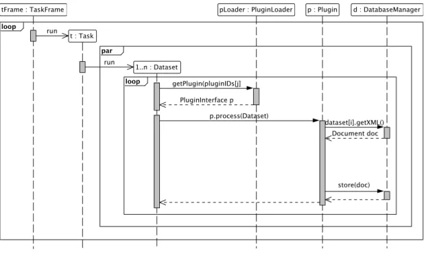
3.4 Task processing: Sequence diagram . . . 35
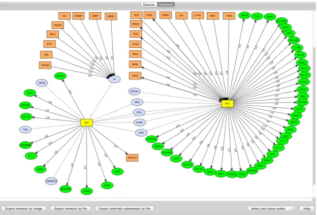
3.5 Network visualization in GRN I . . . 36
3.6 Network visualization in GRN II. . . 37
3.7 Key driver identification pipeline . . . 39
4.1 TFmiR Network View . . . 50
4.2 Distinction between co-targeted and co-regulated subnetworks . . . 51
4.3 Composite FFL motif co-regulation . . . 54
4.4 Cumulative distribution of GO functional semantic scores . . . 56
5.1 Age distribution in MUC Samples . . . 60
5.2 Amyloid-β levels . . . 61
5.3 miRNA expression vs. Braak stage . . . 62
5.4 miRNA Heatmap . . . 64
5.5 Expression before and after processing . . . 65
5.6 Top 12 differentially expressd genes vs. Braak Stage . . . 68
5.7 Overlaps for up- and downregulated genes with known genes . . . . 70
5.8 Overlap with known genes . . . 70
5.9 mRNA Heatmap . . . 71
5.10 Methylation before and after processing. . . 72
5.11 Transcription factor-mRNA network (created with igraph) . . . 75
5.12 miRNA SNP proximity analysis . . . 76
5.13 Differentially methylated regions SNP proximity analysis . . . 78
5.14 Methylated miRNA-gene network . . . 79 xi
A.1 Density of methylated and unmethylated probes before and after
processing . . . 112
A.2 Summed color bias before and after . . . 113
A.3 Color bias for both channels before and after . . . 113
A.4 Density before and after quantile normalization . . . 113
A.5 CpG Intensity before and after processing . . . 114
2.1 Possible outcomes of a hypothesis test . . . 15
3.1 Database Schema . . . 31
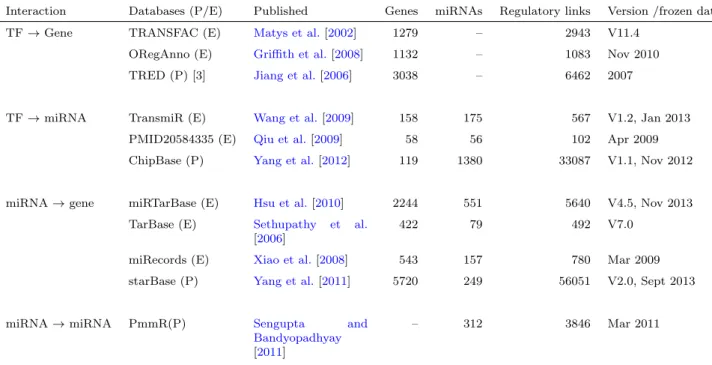
4.1 Databases used in TFmiR . . . 48
4.2 Most significant miRNA nodes in BC disease network . . . 55
4.3 Key drivers in BC network . . . 55
4.4 Drug-targeted key gene nodes . . . 56
5.1 Number of males and females in the example dataset . . . 60
5.2 Call ratios for the doubled samples . . . 63
5.3 Student’s t-test on miRNAs . . . 63
5.4 FDR corrected miRNAs . . . 64
5.5 Number of up- and downregulated genes in test set . . . 66
5.6 Top 30 differentially expressed genes . . . 66
5.7 Top 50 differentially methylated regions, sorted by p-Value . . . 73
5.8 Putative key drivers for Alzheimer’s disease . . . 74
5.9 Functional annotation for the putative miRNA regulated gene targets 80 5.10 Example of the Apogenotype table . . . 81
5.11 Apoprobability table [Raber et al., 2004] . . . 81
5.12 Scoring of different combinations for Similar Network Fusion . . . . 83
5.13 Post-mortem preservation times for MUC samples . . . 83
A.1 Full gene list for AD . . . 107
Introduction
In the last century, biological technology evolved to create a critical amount of data that exceeded the capability to comprehend manually in magnitudes. Thus, a need for structured data storage established and drove the development of bio-logical databases, starting with Margret Dayhoff and theAtlas of Protein Sequence and Structure. This lead to the Protein Information Resource database of protein sequences - today part of the Uniprot consortium [Dayhoff et al., 1976; Dayhoff,
1965]. Meanwhile, her group started the computational analysis of protein struc-tures [Dayhoff,1974,1969]. With Dayhoff’s field of research prevailing and gaining importance up to today, we regard this as the beginning of computational biol-ogy, and bioinformatics. Ever since, the rapidly increasing fund of biological data spans over a respectable amount of databases that hold DNA/RNA sequencing data, methylomes, genotypes, and protein structures.
When evaluating the human genome, more than 1 800 disease associated genes were discovered, enabling the development of a variety of genetic tests for certain conditions [Miklos and Rubin,1996]. However, the knowledge of the genome helps to assess genetic risks but delivers not necessarily deterministic answers for the occurrence of many diseases. Epigenetic regulation mechanisms known as DNA methylation, histone modification, chromatin remodeling and noncoding RNAs, influence which genes actually are expressed and play a major role in cell differen-tiation, growth, and eventually in the pathological history of each individual [Bird,
1986]. For this reason, studies of expression data and epigenetic features together delivered valuable insights.
In order to enhance a comprehensive understanding, databases were designed to embrace a variety of multifaceted biological data with respect to a specific pur-pose, such as The Cancer Genome Atlas (TCGA), which contains gene expression profiling, copy number variation profiling, SNP genotyping, genome wide DNA methylation profiling, microRNA profiling, and exon sequencing.
The availability of such comprehensive datasets rose the question of how to 1
contextualize each other, and lead to the efforts to employ integrated analysis on biological data.
1.1
Biological Data
The translation of biological features on molecular level to generate computation-ally assessable data poses various challenges itself. For example, there is no way to observe the DNA sequence of a human genome in its entirety of over 3 000 Mega-base pairs using a microscope. Thus research focused on methods to ac-complish such tasks, starting with the first practical method presented by Sanger et al.[1977] who amplified DNA using a DNA polymerase with specific terminators for each of the four nucleotides, and enabled to determine the base pair sequence using gel electrophoresis. As one of many examples, DNA sequencing methods enabled structured assessment of biological data and today, various experimental protocols exist to obtain methylomes, expression profiles, DNA/RNA sequences, protein structures and many more.
In the following sections, we outline the methods applicable to obtain the data we studied in the scope of this work.
1.1.1
Enzyme Linked Immunosorbent Assay (ELISA)
The Enzyme Linked Immunosorbent Assay (ELISA) is one of the most established methods to detect the presence of a certain substance in a sample, and its variations share the same concept.
In principle, a liquid sample subjected to test is added to a stationary solid phase with a ligand-specific binding reagent that contains the antigen for a certain antibody or vice versa. Subsequently, a labelled substrate for the antigen is added to the plate and the reaction of non-bound antigens with the substrate induces a color change. The resulting signal is measured using spectrophotometry and allows quantification of the antigen in the studied sample [Voller et al., 1978].
ELISA has been established as a standard for diagnostic tests such as the determination of serum antibody concentrations in HIV patients. In Chapter 5, we study Amyloid-β 40 and 42 measurements obtained with ELISA.
1.1.2
Microarrays
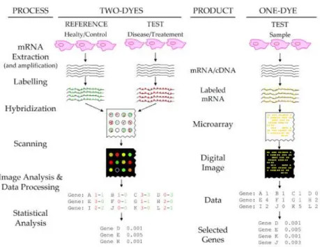
As mentioned before, regulatory mechanisms influence the transcription of the genome. In order to gain an insight into this transcriptional level, genome-wide hybridization arrays were designed and are used today to compare genome-wide features among individuals and tissues. For example, an investigation of samples
from disease patients in comparison with healthy controls may show differences in the expression profiles that hint information on the gene products responsible for the defect. A schematic of a gene expression microarray assay is shown in Figure 1.1. Extracted mRNAs or amplified cDNAs from tissues are labelled with fluorescent markers and hybridized to the array. A laser and a confocal scanner then excite and detect the fluorescent dyes, which yields a digital image from the microarray. Using image processing algorithms, the spot intensities are measured and translated into numerical readings. After estimation and subtraction of the background noise, the final signal is an integer proportional to the concentration of the target sequence for each spot. For two-dye experiments, a ratio of the expression levels of a sample in respect to the reference is determined [Trevino et al., 2007]. A microarray is capable to detect and measure expression levels of thousands of genes in a single experiment.
The microarray technology developed by Illumina in particular is based on oligonucleotides attached to beads that are randomly deposited onto a glass sur-face. Using the address sequence of each bead, bead positions are decoded to determine which bead combination is located in which well [Gunderson et al.,
2004]. Thus, each array has a unique layout file that is used to decode the data when scanning. For gene expression in human samples, Illumina provides an ex-pression BeadChip (HT12v4) that targets more than 47 000 probes with up to 12 different samples per chip.
The design of the beads and therefore the applications of the Illumina BeadChip technology are multifaceted and include arrays used for genotyping, copy-number determination, sequencing, and methylation analysis. The versatility of the plat-form enables to obtain variety of data cost-efficiently, and was used to generate most of the data studied in Chapter 5.
1.1.3
DNA Methylation
DNA Methylation, occuring at the CpG dinucleotide, is probably the most studied epigenetic modification so far. Extensive mapping experiments in different cancers pointed out a key role of DNA methylation in oncogenic development [Boerno et al.,
2010]. When studies showed the potential of methylation-based biomarkers that enhance early diagnosis, prognosis, and classification of cancer, the aim was set to perform epigenome-wide association analysis at reasonable costs.
The Illumina Infinium HumanMethylation 450k BeadChip covers 99% percent of all RefSeq genes with more than 480 000 CpG sites at high coverage with an average of 17 probes per gene. The array includes various functional elements, gene bodies and miRNA promoters are covered as well [Touleimat and Tost, 2012], and generates data for an extensive analysis with a single experiment. As we show in
Figure 1.1: Overview of a microarray experiment for both a comparison experiment with two dyes and a single dye experiment. Left column shows the processing steps, third column the results of each step. Source: Trevino et al.[2007]
Chapter5, we used this data to investigate methylation levels of gene and miRNA promoters together with expression and SNP data.
1.1.4
MicroRNA
Previously, we mentioned DNA methylation assuming a key role in the regulation of gene expression. Other than that, gene regulation may occur at the transcript level. Small non-coding RNAs, microRNAs (miRNA), bind to mRNA transcripts and prevent their translation to protein products. Moreover, targets may recipro-cally influence level and function of miRNAs [Pasquinelli, 2012].
The mutual regulation of miRNAs and target genes is crucial to the under-standing of gene-regulatory mechanisms.
The samples in our Alzheimer study were obtained using the Geniom RT An-alyzer, which is another microarray-based platform. In order to quantify miRNA from the tissue samples, microRNAs are hybridized to microfluidic primers, la-belled. After primer extension, a picture is obtained that is processed subsequently to translate the intensities into a numeric reading.
1.2
Single nucleotide polymorphisms (SNPs)
An investigation of single nucleotide polymorphisms (SNPs) enables to assess ge-netic variations between individuals on a genomic scale. For one position out of every 1 000 nucleotides, the human genome shows a base pair exchange among individuals [Syv¨anen, 2001]. Depending on the location of those SNPs, this may affect an individual in different ways. For example, a SNP that occurs within a gene coding region can change the amino acid composition of the encoded protein and, thus, alternate the structure and function of the product. In fact, many inher-ited disorders are associated with SNPs, such as the Apoallele, which was shown to affect atherosclerosis [Davignon et al., 1988] and plays a role in our studies on Alzheimer’s disease as well.
Apart from the obvious approach to sequence a sample genome, SNPs can be determined using a polymerase chain reaction with allele-specific oligonucleotides or, on larger scales, using microarrays. In our case, the Illumina Human610-Quad beadchip microarray was used to determine the SNPs for the samples in the Alzheimer study.
1.3
Systems Biology
Different biological data represent a collection of systematic measurements. Many-faceted system biology approaches that incorporate such genome-scale experiments have been developed to perform predictive, hypothesis-driven science [Chuang et al., 2010].
1.3.1
Gene regulatory networks
One systems biology strategy in particular aims at the reconstruction of gene regulatory networks (GRNs) from experimental data such as microarray gene ex-pression profiles. The incorporation of more information such as interaction data, genome sequences, or epigenetic information helps to prune and thus to create more concise networks [Hecker et al., 2009].
The construction of regulatory networks and their pruning using other systemic data motivated large parts of the work presented in this thesis. We developed a gene regulatory network plugin based on co-expression data for our software frame-work Mebitoo presented in Chapter 3.3 and published subsequently the breast cancer study described in 3.4. In Chapter4 we introduce the web service TFmiR, that was designed to build a transcription factor-miRNA regulatory network based on differentially expressed genes and miRNAs.
1.4
Similarity Networks
A different approach on data integration was done with networks of individuals [Barab´asi, 2007], for example in Christakis and Fowler [2007] where the authors investigated obesity of individuals and their social network and concluded obesity to spread through social ties.
Likewise, Wang et al. [2014] presented a method to create patient-similarity networks integrating biological data, and merge those into a single network that incorporates the information content of each data source. Thus, this network reflects a condensed representation of the dataset and offers insight into possible complementary characteristics of the different input sources.
Similarity networks and network merging are explained in more detail in section
2.3, and we outline their novel application on Alzheimer’s disease data in Chapter
5.
1.5
Computational Tools for Data Integration
Unsurprisingly, the need for software that enables to create workflows for efficient processing rose together with the amount of biological data available.
Cytoscape, a software environment to integrate biological interaction networks with expression data, was presented by Shannon et al. [2003a] and gained large popularity due to a platform-independent architecture with a graphical user inter-face. Since then, the plugin-based platform received with well over 5000 citations and grew a large developer base that contributed various plugins for data visualiza-tion, ontology analysis, data integravisualiza-tion, clustering, and many more as described inSaito et al.[2012]. However, some of the plugins mentioned are obsolete today, since the platform is under continuous development and was recently rebuild to be future-proof in a major version update to 3.x which is incompatible to 2.x.
Scripting languages on the other hand offer more flexibility to work with bio-logical data. Dialects like Python allow dynamic typecasting and are based on an easy-to-understand syntax in comparison to their regular programming language counterparts and allow for very quick prototyping of data analysis pipelines. The potential was recognized, and groups like Cock et al. [2009] developed libraries that wrapped standard tasks like data import and export for biological data and the execution of BLAST queries or ClustalW alignments on sequences into their package called BioPython.
Statistics in computational biology provide important methods to rule out sig-nificant pieces from the large puzzle of biological data. Designed specifically for the purpose of statistical computing, the R framework naturally provides much of the required functionality. Because R features a packing protocol to extend the
framework, Gentleman et al.[2004] presented their Bioconductor package to close the gap between R and biological data, starting with array-based expression data. Since then, Bioconductor has been extended continuously to allow processing of data from many different biotechnology platforms.
We present our own approach to a software framework for biological data in-tegration and workflow creation in Chapter 3. Both Cytoscape and R were used to develop the pipeline behind TFmiR (Chapter 4), and large parts of the anal-ysis in the Alzheimer’s disease study was carried out using R scripts based on Bioconductor, and various subpackages designed to handle the variation of data sources.
1.6
Complex Diseases
Research has shown that many diseases show a genetic component [Davison et al.,
1994]. Some disorders like sickle cell disease, cystic fibrosis, or Huntington’s disease are linked to mutations in single genes or loci. However, many other disorders are likely to arise due to a combination of genetic factors but are induced by certain lifestyles and environmental factors as well, many of which are yet to be determined. We now know that there are genetic predispositions for certain diseases (such as the Apolipoprotein E (Apo) allele in Alzheimer’s Disease), but a genetic tendency alone proved not be sufficient as definitive predictors for many of them [Craig, 2008].
In the next sections, we describe briefly the complex diseases studied in the scope of this thesis, in particular breast carcinoma and the Alzheimer’s disease.
1.6.1
Breast Cancer
Breast cancer (BC) is the most prevalent carcinoma in females, with one of ten women affected by the age of 80 years and accounts for the second-highest number of deaths of female cancer patients, after lung cancer [Siegel et al.,2014]. Because BC is a genetically heterogenous type of cancer, treatment and prognosis depends on correct classification of the carcinoma at hand [Volinia and Croce, 2013]. Due its complexity, molecular mechanisms and regulatory patterns of the disease are not yet completely understood.
In order to address the complexity with appropriate models,Cava et al.[2014], for example, presented an effective discrimination of cancer types based on a sup-port vector machine classifier combining copy number variations, SNP data, and the expression values of miRNAs, and mRNAs.
In section3.4, we describe our approaches to study BC with regulatory network approaches where we ruled out possible key driver genes and potential drug targets.
Additionally, we present the application of our TFmiR service to build a TF-regulatory network on breast cancer data in section 4.5.
1.6.2
Alzheimer’s Disease
With improved healthcare and life standards in general, the average human life expectancy increased largely, and thus aging and aging-related disease research is regarded increasingly important. Besides cancer that represents in fact a collection of diseases, neurodegenerative diseases pose the most prevalent risk for the elderly. For the most common disorder, the Alzheimer’s Disease (AD), cases double every five years from the age of 65 onwards. Since its discovery in the early 20th century, Alzheimer has been known as a complex disorder that is hard to diagnose in early stages, researchers started to search for possible connections and interactions between different regulatory pathways that point to the mechanism behind the disease.
Medical indications discern between Early-Onset Alzheimers Disease (EOAD) and Late-Onset Alzheimer’s Disease (LOAD). The early-onset form occurs prior to the age of 60-65 years and often even before the age of 55 and is known to be mainly caused by mutations in three genes and inherited in an autosomal-dominant fashion. This familial form is implied by mutations in the genes related to encoding the amyloid precursor protein (APP), as well as mutations both in presenilin-1 and presinilin-2 (PSEN1, PSEN2). In a normal metabolism, APP is processed by the β-secretase 1 (BACE1) and the γ-secretase and is transformed to β-amyloid 40 and 42 (Aβ40, Aβ42) which are then decomposed. However, both peptides show neurotoxic characteristics and plaque accumulations have been found in brain tissues of patients diagnosed with AD as well as with the Down Syndrome. Interestingly, those plaques have been found in patients that suffered from traumatic brain injury [Johnson et al., 2010], which indicates its connection to neurodegeneration not to be limited to AD.
On the other hand, for the LOAD forms that show prevalence in individuals of 60-65 years and above, there are several genes known to be involved in the development of sporadic AD. So far, the gene coding for apoliprotein (Apo) and its genotypes are considered a major factor but not a sufficient marker for diagnostics or prognosis. Statistically, AD patients are more likely to carry the Apo4 allele than the population in general, while Apo2 may be protective [Minati et al.,2009].
Alzheimer’s disease largely affects the episodic and semantic memory as well as it induces noncognitive behavioural changes [Mega et al., 1996]. The temporal lobe - one of the four major brain lobes of the cerebral cortex - has been shown to be largely associated with those traits and thus, with AD [Visser et al., 2002].
In the closing chapter5, we investigate a comprehensive dataset spanning mi-croRNA and gene expression as well as methylome and Amyloid-β levels obtained for 64 samples of temporal lobe tissue from post-mortem patients, of which 39 suffered from Late-Onset Alzheimer’s Disease.
1.7
Outline
This thesis is divided into six chapters. Closing the introduction at this point, the author presents the theoretical part relevant for this thesis in chapter2, where statistical methods and network theory are explained in more detail.
The subsequent three chapters outline major projects the author participated in.
In chapter3, the Mebitoo software framework for data integration and workflow pipelines and the application of the GRN plugin on breast cancer data and their downstream evaluation are presented.
Subject of chapter4is TFmiR, a web service we developed to build regulatory networks based on gene and miRNA expression data. Moreover, we show our studies with TFmiR in respect to breast cancer.
The last project presented in the scope of this thesis is the still ongoing study on Alzheimer’s disease, for which we carried out the analysis for a comprehensive dataset ourselves. Subsequently, we applied the former approaches and addition-ally pursued a different strategy based on patient-similarity networks (Chapter
5).
Finally, the last chapter 6 concludes this thesis with a summary and outlook on future work.
Theory
2.1
Statistical Tests
Statistical hypothesis testing is a common method to draw inference about popula-tions using deviapopula-tions within data from expected values or, in two-sample testing, to compare different groups of samples of a population. For instance, in the scope of this thesis, these are individual markers - such as expression levels for genes and microRNAs or methylated regions, that are tested for significant differences between case and control groups of different diseases.
For each test, one tries to determine a probability for a the dataset given a certain hypothesis is true.
2.1.1
Fundamentals
Classical statistical tests share the same concept:
1. A null-hypothesisH0 and an alternative hypothesis H1 are formulated. Ba-sically, it is hypothesized that a population is different or not different from a certain mean, while the alternative is the antithesis.
2. When calculating a test-statistic, it is determined how probable a property is for the samples in question. As it is in general unlikely to match the exact mean in a statistical test, results are judged by confidence levels. A significance level for the statistic reduces the decision whether or not the null hypothesis is rejected on the so called p-value.
3. If the test statistic fails to satisfy the significance level, it is rejected as being unlikely to hold given the samples.
For the scope of this thesis, a variety of statistical tests has been used which will be introduced in the following sections.
2.1.2
The students’s
t
-test
The t-test finds application when evaluating the mean values of a set of samples to an expected value.
Given a sample X = X1, . . . , Xn of probes independent to each other that
are N(µ, σ2)-distributed with unknown mean µ and variance σ2, the investigated hypothesis is defined as:
H0 :µ=µ0 (2.1)
The test statistic then is defined as shown in equation 2.2:
T :=√n· X¯ −µ0
Sn
(2.2) with the sample variance of the mean Sn= √σn.
This test can be applied for quality assurance, for example to ensure a cohort is within certain specifications: if one is interested if the mean durability time of a set of lightbulbs compared to the specification a manufacturer warrants.
Obviously, the test confidence grows with larger sample sizes.
In case the samples are not normally distributed, non-parametrical test meth-ods are required. For any t-test, there is an alternative non-parametrical test method.
Two-sample t-test
The two-samplet-test is applicable for two samplesX =X1, . . . , Xm ∼N(µX, σ2X)
and Y =Y1, . . . , Ym ∼N(µY, σY2) with homogeneous variance (σ2X =σY2 and both
samples are independent to each other.
Similary as with the one-sample t-test, the null hypothesis is defined alike in equation2.3.
H0 :µX =µY (2.3)
The test statistic in this case is defined in equation 2.4.
T := qX¯m−Y¯n 1 m + 1 n·Sp (2.4) with Sp2 := (m−1)S 2 X,m + (n−1)SY,n2 m+n−2 (2.5)
In order to accept the null hypothesis H0, T should be near to 0, otherwise it is rejected.
If the variance is proven to be heterogeneous instead of homogeneous, e.g. applying a Levene-Test, the t-test is not suitable. An alternative would be the Welch-Test.
In the scope of this thesis, the two-sample t-test is applied for the differential analysis of gene and microRNA expression data as well as methylation analysis.
2.1.3
Hypergeometric Test
The hypergeometric test is based on the hypergeometric distribution and provides a means to compute the statistical significance of specific k probes from n draws from a population sized N with a total of K success probes. In other words, this test is applicable to determine whether the amount of successful draws is over- or underrepresented.
A random variable that is hypergeometrically distributed follows equation2.6:
P(X =k) = K k · N−K n−k N n (2.6)
The p-value is calculated by 1−P
KP(k).
2.1.4
Kolmogorov-Smirnov Test
The Kolmogorov-Smirnov test allows to validate whether or not an observed cu-mulative frequency distribution of samples matches 1.) an expected distribution or 2.) the distribution of another random variable.
To apply this test, observed frequencies are arranged in ascending order, and each cumulative observed frequencyFi is calculated as the sum from f1 up to and including fi. From this, cumulative relative observed frequencies are determined
by:
relFi =
Fi
n (2.7)
with the number of data in the sample n=P
fi.
This distribution then tested against either an cumulative relative expected frequency rel ˆFi, which is calculated alike. The test statistic is calculated first by
the partial calculation
Di =|relFi−rel ˆFi| (2.8)
and
D0i =|rel Fi−1−rel ˆFi−1| (2.9)
Finally, D is the largest value of the largest Di or D0i:
D = max(maxDi,maxDi0) (2.10)
Depending on a desired significance levelα and the amount of samples n,D is rejected when it exceeds a criticalDα,n, for largen approximated by
Dα(2),n =
r
−ln(α/2)
2n (2.11)
as given bySmirnov[1948]. Other computations have been suggested and literature provides tables for those [Miller, 1956;Zar, 2007].
In a summary, the Kolmogorov-Smirnov test allows to search for a maximum deviation between the observed distribution F and the hypothetic distribution ˆF and in case this deviation exceeds a certain threshold, the hypothesis that both curves follow the same distribution is rejected.
In the scope of this thesis, this test has been used to calculate the significance of similar gene frequency within co-regulated and co-targeted genes of motifs in TFmiR.
2.1.5
Multiple Testing Correction
When statistical tests are applied, the probability to find a certain result “by chance” - the p-value usually defines the threshold whether a hypothesis is ac-cepted or rejected. While this works well for few tests, dealing with genomes and microarray experiments leads to several thousand separate hypothesis tests. Ac-cordingly, when testing 20 000 genes with a p-value cut-off at 0.05, still about 1.000 genes may mistakenly be considered significant. The possible outcomes for a hypothesis test are shown in Table2.1.
Thus, the probability of making an error αaccumulates with the number m of hypothesis tests. The probability of not making an error in such a series of tests can be written as:
P(No errors in m tests) = (1−α)m (2.12)
with the probability to make at least one error inm tests 1−(1−α)m. Controlling
the Type I error rate is the aim of thep-value adjustment for multiple testing. In the scope of this thesis we applied the False Discovery Rate correction presented byBenjamini and Hochberg [1995] (BH-FDR).
With the amount of mistakenly accepted hypotheses V - false positives -, the False Discovery Rate is defined as the expected proportion of Type I errors among the rejected hypotheses R:
Actual Situation
Decision H0 True H0 False
Accept H0 Correct decision 1−α Incorrect Decision Type II Error β RejectH0 Incorrect Decision Type I Error α Correct Decision (1−β)
Table 2.1: Possible outcomes of a hypothesis test withα=P(Type I Error)andβ=P(Type II Error). Minimization of Type I errors are the purpose of multiple testing correction methods.
FDR =E(V
R|R >0)·P(R >0) (2.13)
To control false discoveries, this rate is to be kept below a certain thresholdq. For example, if the threshold was 0.10 with 1000 hypotheses rejected for 20 000 genes, less than 100 of those are expected to be false positives.
In general, to control the FDR for m tests at level q, the following steps are applied:
1. Order unadjustedp-values: p1 ≤p2 ≤ · · · ≤pm
2. Identify the test with the highest rankj for which pj ≤ mj ·q
3. Tests of rank 1,2, . . . , j are declared significant
2.2
Graphs
First, fundamentals of graphs and the underlying abstract model is presented.
2.2.1
Fundamentals
On the most abstract level, a graph can be understood as a binary two-dimensional matrix, where rows and columns indicate the source and target elements of a graph and the binary value indicates an existing relation, as shown in equation 2.14.
v1 v2 v3
v1 0 0 1
v2 1 1 0
v3 1 1 0
(2.14)
More intuitively, a graph consists of a set of elements called nodes V =
{v1, v2, . . .}, which are connected via links that indicate connections between
nodes, e.g. with e1 = (v1, v2). The network from 2.14 is translated to a graphical representation in Figure 2.1. Note that, depending on the type of the graph - di-rected or undidi-rected -, the graphical representation may neglect the bidirectional relations inherently whereas the matrix representation is bijective.
Figure 2.1: Example from2.14translated to a graphical representation
The number of links pointing from one node v to all other nodes is defined as the degree of a node.
2.2.2
Network Measures
For analyzing networks in general terms, a variety of centrality measures have been included in the scope of the work presented in Chapter 4.
Degree distribution
The degree distribution defines the probability for each node in a network to have a certain degree k. The trend of the curve in the resulting plot gives information about the characteristics of a network. In an evenly distributed random network
the curve follows approximately a Poisson distribution, while the degree distribu-tion of a scale-free network that is characterized by a few hubs with many links and a large amount of nodes with few links follows a negative power law [Erd˝os and R´enyi,1959; Newman, 2003]. In a biological context, the degree of a node in terms of a protein-protein interaction network can hint at which proteins are key drivers for metabolic processes in a cell.
Average path length
The average path length lG is defined as the average number of steps along the shortest paths (d) between all pairs of all nodes (vi, vj) in a network G with size
n: lG = 1 n·(n−1) · X i6=j d(vi, vj) (2.15)
Intuitively, for a biological interaction network to be efficient in terms of few in-termediate steps, a short average path length indicates efficiency.
Density
The network densityDdenotes the ratio of the number of actual edges E existing in a network G to the number of possible edges, as shown in equation2.16.
D= 2E
N(N −1) (2.16)
Network density has been shown to be an indicator of how robust a model network is to failures. But it has been shown for biological networks that even networks with low average density were robust to node losses. For that reason, Hayes et al.
[2013] distinguished between local and global density and showed for real protein-protein interaction (PPI) networks, that the high local edge density in real world networks contributes to network stability as well.
Diameter
The length of the longest of all shortest paths in a network denotes the network diameter. This value is understood as a characteristic indicator for the linear size of a network.
Transitivity
The network transitivity - or clustering coefficient - is a measure for the clustering in a network.
Usually, one distinguishes between the global and the local clustering coeffi-cient.
The global clustering coefficient is determined by the ratio of the actual num-ber of 3 fully connected nodes to the numnum-ber of connected triplets of nodes in a network, such as shown in equation 2.17
C = no of closed triplets
number of connected triplets (2.17)
The local clustering coefficient measures the clustering coefficient for a single nodei. In words, it is the ratio of all neighbours Ni ={vj :eij ∈E ∧ eji ∈E} of
ithat are interconnected to each other to all possible interconnected nodes, given by the size ki of Ni, 2.18.
Ci =
|{ejk :vj, vk∈Ni, ejk ∈E}|
ki·(ki−1)
(2.18) Measuring the local clustering coefficient of a node in a PPI network, for ex-ample, may indicate the importance of the protein for the metabolism in question.
Closeness
The reciprocal sum of all shortest paths d from a node v to all other nodes in a network gives a measure for the centrality of a node, also called its closeness C, see Equation 2.19.
C(v) = P 1
wd(v, w)
(2.19) This value, relative to the closeness of the other nodes in a network, gives a measure of how relevant a node is in a network in respect to the other nodes.
Note, since this value is an average, it may indicate very proximate distances to only a few nodes (with some very far away) or more similar distances to all nodes. A protein with high closeness could be heavily involved in regulation.
Betweenness
Another measure for the centrality of a node is the betweenness. For any node n and a pair of nodes v1 and v2, the total number of shortest paths linking v1 and v2 passing node n is calculated and related to the overall number of shortest paths between v1 and v2. A high betweenness indicates the importance of a node to maintain connections in a network.
Eigenvector
Other than the degree centrality of a node, the eigenvector centrality assigns a
quality factor to each of the links connected to that node to weight the impor-tance of the respective link. This factor is obtained by calculating the eigenvalues for the adjacency matrix and assigning those as weights. Intuitively the higher the eigenvector value of a certain node scores implicates a higher weight for the neighbouring nodes.
In a biological sense, a high eigenvector centrality protein is likely to be in-teracting with other important proteins, together resembling a critical part of an metabolic pathway.
In the context of drug discovery and a differential analysis of disease and healthy population, eigenvector centralities may help to reveal potential targets.
2.2.3
Minimum dominating sets
Originally developed to minimize resource allocation for wireless networks, Rai et al. [2009] presented an algorithm to find a minimum connected dominating set that represents the most efficient way to connect through the hubs in a network.
A connected dominating set (CDS)C of a graph Gis the set S that induces a connected graph, and the minimum connected dominating set (MCDS) is the set with the minimal number of links necessary.
Because the problem is known to be NP-hard, it requires heuristics to solve a MCDS search in reasonable time [He et al., 2011].
For an adjacency matrix of a graph we define a vector X with Xi for each
nodei= 1, if the node has been recognized as a key node and 0 otherwise. Then, solving the optimization problem shown in equation2.20yields the dominating set of nodes. min n X i=1 Xi subject to∀i n X i adj (i, j)X(j)≥1 (2.20)
In collaboration with Maryam Nazarieh, the author adapted this algorithm to identify key driver nodes for regulatory networks, and we provide this functionality our webservice described in Chapter 4.
2.2.4
Network Motifs
Moreover, when it comes to understand network characteristics, an important question is whether the network can be decomposed into building blocks. This was shown in the transcription regulation of the bacterium E. Coli by Huerta et al. [1998] andThieffry et al. [1998].
2.2.5
Motifs in TF-miRNA interaction networks
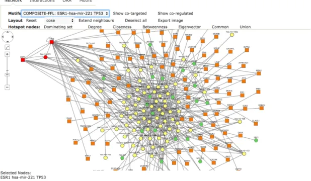
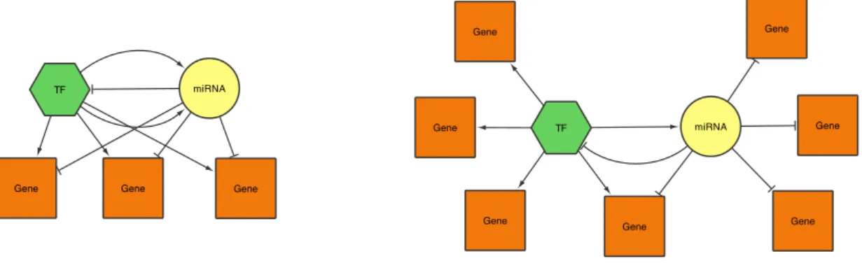
Key functional modules in a regulatory network are represented by Feed Forward Loops (FFLs). These have been shown to be important patterns in transcriptional regulation networks that are responsible in normal cell functions and diseases alike [Milo et al., 2002]. In Figure 2.2, the relevant motifs are shown.
Figure 2.2: Schematic of the four motifs investigated in TFmiR, as shown inHamed et al.[2015a]
Co-regulation feed forward loop (CR-FFL)
The co-regulation FFL resembles the regulation of a target gene by a transcription factor as well as the repression of the same gene by a miRNA.
miRNA feed forward loop (miRNA-FFL)
If a miRNA represses both the target gene and the TF which regulates the target gene as well, the miRNA-FFL pattern applies.
Transcription factor feed forward loop (TF-FFL)
This describes the regulation of expression of both miRNA and a target gene as well as the miRNA repression of the target gene.
Composite feed forward loop (C-FFL)
The composite FFL describes the most dense interaction between the three com-ponents. The transcription factor regulates both a miRNA and a target gene and the corresponding miRNA represses both the TF and the target gene.
2.2.6
Statistical evaluation
First, the hypergeometric test shown in Section 2.1.3 is applied to identify signifi-cant transcription factor and microRNA pairs that both regulate the same target:
p−value = 1− x X i=0 k i M−k N−i M N (2.21)
with k the number of targets of the miRNA in question, N the number of genes
regulated by a certain TF and x the number of common targets of both, and
M the number of all genes regulated by miRNAs and TFs in the databases we
queried. After applying the BH FDR correction (see 2.1.5), only remaining pairs with adjusted p-value <0.05 were retained as significant.
2.2.7
Motif search algorithm
Since the motifs are similar and share an incremental structure, instead of searching for each motif individually, the algorithm could be applied based on the existing links in the network in such manner that all motifs are discovered during a single iteration over the whole set of edges in the network, which made the processing highly efficient.
Since all motifs share outgoing edges for a transcription factor, all edges that originate from a TF are identified. Then, for those edges targeting a gene, the gene is subsequently tested for miRNA regulations (edges incoming from miRNAs). For those microRNAs, the interactions to the original TF are checked and subsequently the motif can be classified as one of the four motifs defined above. Algorithm 1
shows a pseudocode listing of the motif search.
The motif search algorithm was implemented on network level using Java and Cytoscape.
Algorithm 1 Motif search
1: procedureMotifSearch
2: MotifsList motifs
3: fore: edges in network ndo
4: interactionType←InteractionType.determine(e)
5: if interactionType.getSourceType() == ’TF’then
6: Node tf←e.getSource()
7: if interactionType.getTargetType() == ’GENE’then
8: Node gene←e.getTarget()
9: forEdge other : getAdjacentEdgeList(gene, INCOMING)do
10: InteractionType otherType = InteractionType.determine(other)
11: if otherType == ’miRNA’then
12: Node miRNA←other.getSource()
13: if n.containsEdge(miRNA, tf)
14: ∧n.containsEdge(tf, miRNA)
15: ∧n.getNeighbors(tf, OUTGOING).contains(miRNA)
16: ∧n.getNeighbors(tf, INCOMING).contains(miRNA)then
17: MotifType←COMPOSITE-FFL
18: else if n.containsEdge(miRNA, tf)
19: ∧n.getNeighbors(tf, INCOMING).contains(miRNA)then
20: MotifType←miRNA-FFL
21: else if n.containsEdge(tf, miRNA)
22: ∧n.getNeighbors(tf, OUTGOING).contains(miRNA)then
23: MotifType←TF-FFL
24: else
25: MotifType←CO-REGULATION
26: motifs.add(createMotif(motifType, tf, miRNA, gene))
returnmotifs
2.2.8
Motif significance
In order to validate the significance of the motifs found in a certain network, we implemented a comparison to their occurrence in random networks based on the original network layout.
Network randomization
In order to retain the stronger attachment of key driver nodes, we decided to apply a degree-preserving randomization algorithm. For a network with L edges, two edges e1 = (v1, v2) and e2 = (v3, v4) are randomly chosen for 2×L from all edges E of the network and rewired such that start and end nodes are swapped, i.e. e3 = (v1, v4) ande4 = (v3, v2) if{e3, e4} 6∈E.
Random network comparison
We calculate thep-value for a motif as follows:
p−value = Nh
Nr
which denotes the ratio of a certain motif to be acquired more or equal times in the tested networkNh to the number of created random networks, withNr = 100
in our specific case.
Moreover, we calculate the Z-score for each motif type to investigate by how many standard deviations the observed motif was above or below the mean of random ones, defined as:
Z−score = No−Nm
σ (2.23)
with number of motifs observed in the real network No and Nm, σ the mean and
standard deviation of motif occurrence in the 100 random networks created.
2.3
Similarity Network Fusion
In order to investigate the individual datasets provided by Riemenschneider et al (see Chapter 5), we applied Similarity Network Fusion (SNF), a method proposed byWang et al.[2014] which allows to integrate several different datasets retaining information about the individual samples. This approach was originally developed for computer vision and image processing by Wang et al. [2012].
2.3.1
SNF algorithm
The idea is to construct a graph G = (V, E) that resembles a patient similarity network for each dataset. The vertices V =v1, . . . , vn correspond to the patients,
while the edges E are weighted by how similar the patients are. For continous variables, with the Euclidian distance ρ(vi, vj) between two patients i and j, the
weight for this edge is determined by a scaled exponential similarity kernel defined as: W(i, j) = exp−ρ 2(v i, vj) µi,j (2.24) with an empirically set hyperparameter µ and i,j as a means to eliminate the
scaling problem, defined as:
i,j =
¯
ρ(vi, Ni) +ρ(vj¯, Nj) +ρ(vi, vj)
3 (2.25)
with ρ(vx¯, Nx) being the average value of distances between vx and each of its
neighbors.
For discrete variables, the authors suggested using the chi-squared distance measure which in our work has been used to incorporate Apogenotypes later on. As the intention is to integrate different measured datasets, a fused matrix from the individual patient similarity networks had to be computed.
For this, a normalized weight matrix P =D−1W is calculated with the matrix
D(i, i) = P
jW(i, j) such that
P
jP(i, j) = 1. This is called a full kernel on the
vertex set V. To account for the normalization for self-similarities, the normaliza-tion is adapted for wheni=j:
P(i, j) = ( W(i,j) 2P k6=iW(i,k), j 6=i 1 2, j =i (2.26)
Now, to measure the local affinity of a nodevi to all its neighborsNi (including
vi) in G, a k-nearest neighbors method applied as:
S(i, j) =
( W(i,j)
P
k∈NiW(i,k), j ∈Ni
0, otherwise (2.27)
That way, non-neighboring nodes are set to zero similarity values. While the matrix P contains full information about the similarities, S considers only the similarity to the k most similar patients for each patient.
The network fusion starts withP as initial states and incorporatesS as a kernel to model the local structure of the graphs.
For m different datasets, similarity matrices W1, . . . , Wm are computed using
equation2.24, likewise Pn and Sn from equations 2.26 and 2.27.
The idea behind SNF is to iteratively update the similarity matrix correspond-ing to each datatype. Assume two data sets for which two status matricesP1 and P2 have been calculated (iteration t = 0). The update process for both matrices is defined as:
Pt1+1 =S1×Pt2×(S1)T (2.28)
Pt2+1 =S2×Pt1×(S2)T (2.29)
with P1
t+1 and Pt2+1 the status matrices for the first and second datatype after t iterations, respectively. In that manner, status matrices are updated each time step in an interchanging fashion.
The final matrix after t steps is defined as:
Pc= P
1
t +Pt2
2 (2.30)
In order to reduce noise, the method can be modified to include only common neighborhoods Ni of a node vi: Pt1+1(i, j) = X k∈Ni X l∈Nj S1(i, k)×S1(j, l)×Pt2(k, l) (2.31)
As a result, if two nodesvi and vj share common neighbors in both similarity
matrices, they are likely to be part of the same cluster. Also, if two nodes are not similar according to one dataset, the similarity within other datasets propagates into the other matrices during the fusion. After each iteration, the normalization from Equation2.26is applied after each iteration step to ensure that a node always is more similar to itself than to others and to guaranteee that the final network is full rank, i.e. a regular matrix with non-zero eigenvalues. This is important to apply classification and clustering to the final network.
The extension to more than two datasets is defined as an generalized version of Equations 2.28 and 2.29: pv =Sv× P k6=v Pk m−1 ×(S v )T, v = 1, . . . , m (2.32)
The resulting fused matrix Pc can be used for clustering and classification of
the nodes.
2.3.2
Network Clustering
In order to identify possible subtypes in a fused network graph withnsamples and mmeasurements, we try to determine clusters of samples. A label vector is defined such that for each samplexi, a vector is defined such that for each possible subtype
k, yi(k), the value 1 and 0 is assigned depending on whether or not the sample
belongs to the respective subtype. Thus, the partition matrix Y = (yT
1, y2T, . . . yTn)
describes the clustering scheme.
With SNF, spectral clustering is used to identify the network clusters by min-imizing the RatioCut [Ng et al., 2001; Wei and Cheng, 1989] by solving the opti-mization problem defined as:
min
Q∈Rn×CTrace (Q
TL+Q)s.t.QTQ=I (2.33)
with the scaled partition matrixQ=Y(YTY)−12, the normalized Laplacian matrix
L+ = I −D−1
2W D− 1
2 with similarity matrix W and the network degree matrix
D (with 0 diagonal elements). This method has been shown to incorporate the global network structure [von Luxburg, 2007].
2.3.3
Normalized Mutual Information
The normalized mutual information (NMI) is a measure to evaluate a clustering against the number of clusters. The measure is defined as the ratio of the mutual information to the entropy H of clusters and classes, respectively.
The mutual information with clusters W and classes C is defined as: I(W, C) =X k X j P(wk∩cj) log P(wk∩cj) P(wk)·P(cj) (2.34)
withP(wk) the probability for an element to be in clusterwk,P(cj) the probability
being classcj and P(wk∩cj) the intersection of both.
The entropyH, a measure for the uncertainty of the respective outcomes for a probability function, is calculated as follows:
H(W) =−X
k
P(wk) logP(wk) (2.35)
and analogously for the classes C.
Finally, the normalized mutual information can be written as:
NMI(W, C) = I(W, C)
[H(W) +H(C)]/2 (2.36)
As bothH(W) and H(C) each are an upper bound to I(W, C), the dominator is divided by 2 to obtain values between 0 and 1 for the NMI score.
As the entropy increases with the number of clusters, the NMI score tends to value fewer clusters higher than a large number of clusters and, thus, allows to compare clusterings with different numbers of clusters.
We used NMI to compare the clusterings obtained with the similarity network fusion method using different combinations of data input sources.
Mebitoo - an Extensible Software
Framework for Bioinformatics
Analysis Workflow
Automatization
This chapter introduces the software framework Mebitoo. This software is a col-loborative project for which the author contributed the mainframe software and plugin architecture, while additional plugins have been developed and used in various Bachelor projects supervised by the author. This work was published in
Spaniol et al. [2015]. The case study on breast cancer describes a collaboration with Johannes Trumm and Mohamed Hamed that aimed at integrating regulatory network analysis.
3.1
Introduction
Initially, with Mebitoo we developed a software with the intention the perform analysis on membrane protein sequences [Spaniol, 2009]. However, applications in computational biology require to target a wider range of research fields beyond se-quence analysis. When aiming at a more extensive view at biological data to gain a better understanding of complex processes, it has become popular to integrate data from various sources and perform a comprehensive analysis. For instance, in the field of complex disorders such as Alzheimers disease, the pathogenic factors have remained largely unexplained so far and it has been suggested that integra-tion of various data such as gene expression, DNA methylaintegra-tion, single nucleotide polymorphisms (SNPs) and protein level measurements may lead to a better un-derstanding of the disease [Rhinn et al.,2013; Zhang et al., 2013].
3.1.1
Related work
In the last years, various tools to pipeline data analysis have been presented. Web-based software like the Galaxy tool [Goecks et al.,2010] allow for interactive analysis of sequencing data. Users upload sequences to a remote public server or set up a local workspace environment. The software allows stepwise processing of generated data so that the workflow is highly adaptable to different types of analysis intended. Programmers can also extend the software using their own plugins to customize workflows with Python scripts. Another well-known tool is Geneious [Kearse et al., 2012], which is a Java Desktop application that allows for a variety of sequence manipulation analysis and may also be extended by own workflows or plugins.
While Galaxy performs on webserver basis that has the possibility to scale for large computational efforts, Mebitoo as desktop application does not require system administration knowledge or access to a server infrastructure and still qual-ifies for working with sensitive (e.g. clinical) data. On the other hand, Geneious emerged to become the standard software for many applications and excels as tool for the daily work with biological data and features a plugin development API that exceeds the concise plugin architecture of Mebitoo in complexity.
3.1.2
Motivation
With Mebitoo we developed a desktop software framework that enables for the implementation of a variety of analysis tools with the intention to minimize the overhead of plugin development. That way, the software is amenable to extensions by developers who can focus on implementing new methods while the framework provides the interface for data management and interaction with other modules. To manage module interaction, users are enabled to define tasks that automatically execute a variety of customized workflows. Mebitoo is set apart from other software by the ability to process arbitrary data supported by a database management system and XML (see Section 3.2.2), a task manager to enable workflows within a graphical user interface (Section 3.2.5) and the extendability with customized method plugins (Section3.2.4).
3.2
Design
Mebitoo is a software application suite written in Java that is based on the Net-beans Rich-Client platform (RCP) project backed by Oracle.
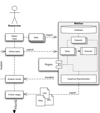
XML Researcher Sequences import Mebitoo Database Plugins Obtain sequences W orkfl ow
Define tasks submit
Analyse results redefi ne Executor Tasks CSV Graphical Representation Datasets PNG export visualize Further usage Data Data
Figure 3.1: Mebitoo framework overview. The core (grey) provides the basic functionality for data import and task definition and execution as well as the plugin interface. Externally devel-oped plugins can be mounted by the framework and executed by a task manager.
3.2.1
Core Module
The core module provides the framework for data management and processing. It (1) implements data import and storage, (2) defines the plugin system that provides an interface to communicate with extensions, and (3) provides a task management that is used to define and queue tasks that process the datasets. A framework overview is shown in Figure 3.1.
The data storage layout realized in Mebitoo uses the HSQL database engine and allows to store either collections of sequences as datasets or additional arbitrarily structured data as XML-documents.
The plugin structure is based on the module architecture provided by the Net-beans Rich-Client platform. It supports a concise abstract interface and provides plugin templates which can be easily adapted by developers to execute customized methods.
Tasks are defined as relations between plugins and datasets, that can be ob-jected to parallel processing. Each task can be queued and finally submitted as a single processing job.
3.2.2
Database Design
Concerning the database itself, we provide a concise concept with few tables that are not allowed to be altered by plugin developers.
In order not to limit a plugin developer on the database concept presented here, if an application requires to apply custom data structures as applied when we worked with regulatory networks, the database design can be extended by plugins themselves. To maintain consistency for the core module, Mebitoo runs a database check at every startup. When working with separate projects, Mebitoo features an option to swap between different databases.
Entity Relationship Model
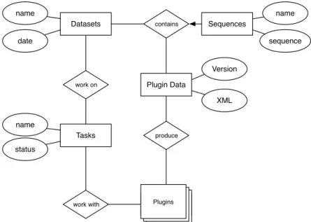
The diagram in Figure 3.2 shows a simplified entity relationship model, which omits the primary and foreign key attributes. Those have to be added for each entity and relation to obtain a complete model when the database is actually implemented.
Each entity and relation is modeled in the database, except for the plugins. Those are loaded from the file system dynamically. Instead of modeling a plugin representation within the database that requires to synchronize between database and plugins, we use the plugin identifiers (e.g. org.mebitoo.plugin.aligner) as symbolic foreign keys and use them to directly retrieve plugins from the module system service provider.
Any dataset may contain an arbitrary amount of sequences, but no sequence can belong to more than one dataset. A task can be linked to any dataset and plugin, but only once to every entity. This restriction is a key predicate for the task execution model. A plugin data entity has to be unique for each dataset and plugin – regardless of the plugin version – but any dataset can have as many data entries as there are plugins and a plugin may also produce XML files for any dataset.
Schema
The final database design applies to the schema shown in Table3.1.
3.2.3
Dataset Structure
In its abstract sense, a dataset in Mebitoo is a collection of data that belongs to one certain entity. For example, a dataset could consist of a single sequence, one sample of sequences from a cohort, or an entire cohort itself. Whenever a task is processed, the dataset as a whole is passed to the processing. Thus, it depends on the modules how to interpret the plugin data associated with a certain dataset.
Datasets contains Sequences name date name sequence Tasks work on name status Plugins work with Plugin Data XML produce Plugins Version
Figure 3.2: A compact Entity Relationship model of the Mebitoo database.
Table 3.1: Database Schema
Datasets (id: int,name: string, date: bigint) Sequences (id: int,dataset id: int,
name: string, sequence: string)
Tasks (id: int,name: string,
date: bigint,status:int)
Plugin Data (id: int,dataset id: int, plugin id: int,
plugin version: string, date: bigint, xml:CLOB) Task Plugins (id: int,task id: int;plugin id: int)
Task Datasets (id: int,task id: int;plugin id: int)
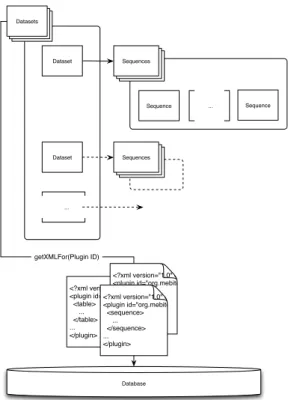
We defined the plugin data as XML documents that are stored as OTHER objects in the HSQL database. Basically an XML document is created for each dataset and plugin tuple. Thus, when a plugin and dataset are selected, the dataset container forwards the request to the database interface and builds a JDOM from the XML file on-the-fly.
Other than dataset, sequence, and task information, the plugin data is not read from the disk until required but the plugin data table is realized as a cached table. This affects the performance negatively because reading data from the hard disk