Generic Market Models

Generic Market Models

1

Raoul Pietersz

Erasmus Research Institute of Management, Erasmus University Rotterdam, P.O. Box 1738, 3000 DR Rotterdam, The Netherlands (e-mail: [email protected]) and Product Development Group (HQ7011), ABN AMRO Bank, P.O. Box 283, 1000 EA Amster-dam, The Netherlands.

Marcel van Regenmortel

Product Development Group (HQ7011), ABN AMRO Bank, P.O. Box 283, 1000 EA Amsterdam, The Netherlands (e-mail: [email protected]).

Abstract. Currently, there are two market models for valuation and risk man-agement of interest rate derivatives, the LIBOR and swap market models. In this paper, we introduce arbitrage-free constant maturity swap (CMS) market mod-els and generic market modmod-els featuring forward rates that span periods other than the classical LIBOR and swap periods. We develop generic expressions for the drift terms occurring in the stochastic differential equation driving the forward rates under a single pricing measure. The generic market model is par-ticularly apt for pricing of Bermudan CMS swaptions, fixed-maturity Bermudan swaptions, and callable hybrid coupon swaps.

Key words: market model, generic market models, generic drift terms, hybrid products, BGM model

JEL Classification: G13

Mathematics Subject Classification (2000): 91B28, 60H30, 60G44

1_{Date: 13 January 2005. We are grateful to Antoon Pelsser for comments and to Russell} Barker for simplifying the proof of Theorem 1. We are particularly grateful to Mark Joshi, for pointing out the possibility of reduced factor drift calculations in the swap market model, which eventually led us to Algorithm 3 for CMS market models.

1

Introduction

Currently, there are two types of market models for valuation and risk manage-ment of interest rate derivatives, which are the LIBOR and swap market models of Brace, G¸atarek & Musiela (1997), Jamshidian (1997), Musiela & Rutkowski (1997) and Miltersen, Sandmann & Sondermann (1997). In this paper, we in-troduce generic market models featuring forward rates that span periods other than the classical LIBOR and swap periods. The generic market model gener-alizes the LIBOR and swap market models. We derive necessary and sufficient conditions for the structure of the forward rates to span an arbitrage-free econ-omy in terms of relative discount bond prices, at all times. We develop generic expressions for the drift terms occurring in the stochastic differential equation (SDE) driving the forward rates under a single pricing measure. We show how the instantaneous correlation of the generic forward rates can be calculated from the single instantaneous correlation matrix of forward LIBOR rates. These re-sults are sufficient for implementation of calibration and pricing algorithms for generic market models.

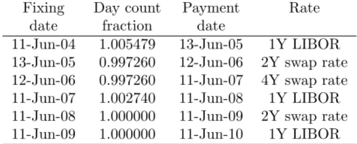
Generic market models are specifically designed for the pricing of certain types of swaps. In particular, we will consider constant maturity swaps (CMS) and hybrid coupon swaps. An interest rate swap is an agreement to exchange, over a specified period, interest rate payments, at a specified frequency, over a specified underlying notional that is not exchanged. In a plain-vanilla swap, the floating interest rate is the LIBOR rate. Aconstant maturity swap pays not the LIBOR rate but instead a swap rate with specified tenor, fixed for all payments in the CMS swap. The payment frequency remains unchanged however. Ahybrid coupon swap is a swap that features a floating payment schedule, designating the nature of each of the floating payments. The nature of the floating payment can be that it is determined by either a LIBOR rate with varying maturity or a swap rate with varying tenor. An example of such a payment schedule has been given in Table 1. Additionally, the function that transforms the LIBOR or swap rate into a cash flow may even be not entirely linear, for example, capped, floored or inverse.

The above swaps may have the feature that the swaps can be cancelled. Such versions are deemed cancellable swaps. To hold a cancellable swap is equal to holding a swap and an option to enter into the very same swap but with reversed cash flows2_{. The latter option is called acallable swap. In this paper we will}

also be concerned with the pricing of callable and cancellable CMS and hybrid coupon swaps. There are two types of callable swaptions: fixed-maturity or

co-terminal. A co-terminal option allows to enter into an underlying swap at several exercise opportunities, where each swap ends at the same contractually determined end date. The swap maturity becomes shorter as exercise is delayed. In contrast, for the fixed-maturity version, each underlying swap has the same contractually specified maturity and the respective end dates then differ.

The main outset of the paper is that a model is deemed to be proper for

valu-2_{Some readers might not be familiar with ‘callable’ and ‘cancellable’ swaps and might prefer} to think of swaps and options thereon.

Table 1: Example of a hybrid coupon swap payment structure for the floating side. Date roll is modified following and day count is actual over 365.

Fixing Day count Payment Rate

date fraction date

11-Jun-04 1.005479 13-Jun-05 1Y LIBOR

13-Jun-05 0.997260 12-Jun-06 2Y swap rate 12-Jun-06 0.997260 11-Jun-07 4Y swap rate

11-Jun-07 1.002740 11-Jun-08 1Y LIBOR

11-Jun-08 1.000000 11-Jun-09 2Y swap rate

11-Jun-09 1.000000 11-Jun-10 1Y LIBOR

ing a certain callable or cancellable swap, if the volatility of a rate that appears in the contract payoff has been calibrated correctly to the market volatility. The concept is best illustrated by example. In the case of the hybrid coupon swap of Table 1 at the valuation date 11 June 2004, we would want to calibrate ex-actly to the volatilities of the 1Y ×2Y swaption, 2Y ×4Y swaption, 3Y caplet, 4Y ×2Y swaption and 5Y caplet. In contrast, for a cap one would calibrate to the volatilities of the 1Y, 2Y, 3Y, 4Y and 5Y caplets. For a co-terminal Bermu-dan swaption, to the volatilities of the 1Y ×5Y, 2Y ×4Y, 3Y ×3Y, 4Y ×2Y

and 5Y ×1Y swaptions. When employing a LIBOR market model to value a cap, the model would feature the following 1Y forward LIBOR rates: 1Y, 2Y, 3Y, 4Y and 5Y. If a swap market model would be used to value the Bermu-dan swaption, it would feature the 1Y ×5Y, 2Y ×4Y, 3Y ×3Y, 4Y ×2Y and 5Y ×1Y forward swap rates. For both LIBOR and swap market models, the canonical interest rates are simply equipped with the corresponding canonical volatilities, allowing for an efficient and straightforward calibration. Obviously, to straightforwardly calibrate a market model for the hybrid coupon swap of Table 1, and callable or cancellable versions thereof, the model would have to feature the forward swap rates 1Y×2Y, 2Y×4Y, 4Y×2Y, and the 1Y forward LIBOR rates at 3Y and 5Y. Up to now, whether a model containing such rates would be arbitrage-free is not well-known. To our knowledge, generic methods for deriving the arbitrage-free drift terms for the SDE driving the various for-ward rates have not been developed yet. In this paper, we develop such generic theory.

In terms of practical relevance, the generic market model technology is valu-able to financial institutions that aim to trade in CMS Bermudan swaptions or callable hybrid coupon swaps. As such, their costumers might require any se-quence of various maturity LIBOR or swap rate payments in the tailored exotic derivatives that they demand for their business. In this paper, we show that a generic implementation of the resulting drift terms is feasible in practice, thereby enabling proper pricing and hedging of such hybrid coupon swaps.

A further motivation for the theory in this paper is that the idea of generic market models is not new to the finance literature, since it has already been

suggested by Galluccio, Huang, Ly & Scaillet (2004). These authors discuss what they call theco-sliding (commonly referred to as ‘LIBOR’) andco-terminal

(commonly referred to as ‘swap’) market models. The class of co-sliding market models corresponds to our class of CMS market models, but ours is defined differently. Galluccio et al. (2004) show that the only admissible co-sliding model is the LIBOR market model. Interestingly, we show that there aren arbitrage-free CMS market models associated with a tenor structure withnfixings, and the LIBOR and swap models are two special cases of these CMS models. In addition to thenCMS models, we introduce generic market models, extending the number of arbitrage-free market models ton!. Also, Galluccio et al. (2004) discuss theco-initial market model, but this model does not fit into our dynamic market model framework. Moreover, in contrast to Galluccio et al. (2004), we derive generic expressions for the drift terms of the forward rates, for all n! models (thus for LIBOR, swap, CMS and generic models).

An alternative way of calibrating a model to the relevant volatility levels, is to take a LIBOR market model, and derive generic approximate expressions for the volatility of various forward rates. Such a procedure, for the specific case of calibration of the LIBOR model to swaption volatility, has been investigated in J¨ackel & Rebonato (2003), Joshi & Theis (2002), Hull & White (2000) and Pietersz & Pelsser (2004). The advantage of the generic market model specifica-tion is that the relevant volatility funcspecifica-tions can be directly specified. Moreover, the development of the theory of generic market models is justified already by the additional insight into the workings of LIBOR and swap market models.

We mention three areas of market model theory to which the generic mar-ket model approach extends. First, generic models may also be used in multi-currency market models, see Schl¨ogl (2002). Second, a numerical implemen-tation of a generic model may utilize drift approximations, see, for example, Hunter, J¨ackel & Joshi (2001) and Pietersz, Pelsser & van Regenmortel (2004a,

b). Third, generic models may be equipped with smile dynamics. The volatil-ity smile is the phenomenon that for European options different Black (1976) implied volatilities are quoted in the market when the strike of the option is varied. The derivation of generic market models in this paper does not make any assumptions on the instantaneous volatility. As a result, smile-incorporating models, such as the displaced diffusion (Rubinstein 1983), and constant elastic-ity of variance (CEV) (Cox & Ross 1976) models, can be readily applied to the generic market model framework. An application of the CEV specification to the LIBOR market model can be found in Andersen & Andreasen (2000).

Finally, for an in-depth overview of pricing models for interest rate deriva-tives, the reader is referred to Rebonato (2004).

An outline of the paper is as follows. First, preliminaries are introduced. Second, necessary and sufficient no-arbitrage conditions on the structure and values of the forward rates are derived. Third, generic arbitrage-free drift terms for the forward rates are derived under a change of measure in a market model setting. Fourth, the numeric efficiency of the generic drift term calculations is discussed. Fifth, the issue of calibrating generic market models to correlation is addressed. Sixth, we end with conclusions.

2

Preliminaries

Consider tenor times or atenor structure 0 =:t1 < · · ·< tn+1 and day count

fractions αi, over the period [ti, ti+1], for i = 1, . . . , n. Suppose traded in the

market is a set ofmforward LIBOR or swap rate agreements that are associated with that tenor structure3_{. Initially,mmay be different fromn, but in Theorem}

1 we show that it makes sense, from an economic point of view, to consider only

m=n. The set of associated forward swap agreements is administered by a set of pairs

E = n²j=

¡

s(j), e(j)¢; j= 1, . . . , m; s(j), e(j) integers ;

1≤s(j)< e(j)≤n+ 1o. (1)

Here s(j) ande(j) denotestart andend of the forward swap agreement. The above set expression forEsimply designates that there aremassociated forward swap agreements, that each forward swap agreement starts and ends on one of the tenor times and that a start is strictly before an end. If the start s and endeof two forward swap agreements²(1)_,²(2) _{are equal, then²}(1) _and²(2) _are

considered equal, thereby a priori excluding the possibility of different forward rates for the same forward swap agreement. Note also that different payment frequencies for a given swap period are not allowed. The value of the forward rate associated with²j is denoted byfj. Forward ratefj may, and shall, in the

course of our paper, depend on time,fj =fj(t). The associated forward swap

agreement is defined as follows. At timests(j)andte(j)the agreement starts and

ends, respectively. The agreement is partitioned by thee(j)−s(j) accrual periods [ts(j), ts(j)+1], . . . , [te(j)−1, te(j)]. The LIBOR rate is recorded at the start of each

accrual period. If the accrual periods are indexed byi=s(j), . . . , e(j)−1, then the LIBOR-observation time isti, the maturity of the LIBOR deposit isti+1−ti,

and the observed LIBOR rate is denoted by `(ti). If forward swap agreement

j has been entered into at time t∗ _{at rate f}

j(t∗), then the fixed and floating

payments are αifj(t∗) and αi`(ti), respectively. We assume liquid trading in

the market at timest∗ _=t

1, . . . , tn of those forward swap agreements ²∈ E for

whichts(j)≥t∗. In other words, there is trading in a forward swap agreement

if the agreement has not yet started or is about to start. We assume the cost of entering into any forward swap agreement at any tenor time to be zero.

The forward swap agreement structures of the LIBOR and swap market models fit into the framework of (1). For the LIBOR market model (LMM),

ELMM = {(1,2),(2,3), . . . ,(n, n+ 1)}. For the swap market model (SMM),

ESMM={(1, n+ 1),(2, n+ 1), . . . ,(n, n+ 1)}. We introduce here a third kind of

market model, associated with theq-period CMS rates. We name it theCMS(q) market model, forq= 1, . . . , n, and it is defined byECMS(q)={(1,1 +q),(2,2 + 3_{The frequency of the floating payments is restricted to one payment per fixed-payment} period, but this is only for ease of exposition. In practice, this assumption may be relaxed and the theory follows through unchanged for any positive whole number of floating payments per fixed-payment period.

q), . . . ,(n−q+ 1, n+ 1),(n−q+ 2, n+ 1), . . . ,(n, n+ 1)}. Note that forq= 1 andq=nwe retain the LIBOR and swap market models, respectively.

The structure of these market models can be specified equivalently as follows, too. There exists an enumeration ²j = (s(j), e(j)), such that, for the LIBOR

model,s(j) =j,e(j) =j+ 1. For the swap model,s(j) =j, e(j) =n+ 1. For the CMS(q) model, s(j) =j,

e(j) =j+q (j = 1, . . . , n−q+ 1), e(j) =n+ 1 (j =n−q+ 2, . . . , n). (2)

2.1

Absence of Arbitrage

Associated with the tenor structure we also considerdiscount bonds. A discount bond is a hypothetical security that pays one unit of currency at its maturity. The price at timet of a discount bond maturing at timeti is denoted bybi(t).

Note that there aren+ 1 discount bonds and that we necessarily havebi(ti) = 1

for i = 1, . . . , n+ 1. The latter is just saying that the cost of immediately receiving one unit of currency is one unit of currency. The time-t1 discount

bond prices are sometimes simply denoted bybi rather than bybi(t1).

In terms of price consistency among the discount bonds, forward swap agree-ments, and LIBOR deposits, we require some form of absence of arbitrage. We follow Musiela & Rutkowski (1997), in which two forms of no-arbitrage are intro-duced. First, a weaker notion of no-arbitrage is the usual no-arbitrage condition in a pure bond market. Second, a stronger notion of no-arbitrage assumes, in addition, that cash is also available in the market, which means that money, not stored in a money market account, can be carried over at zero cost. The stronger form of no-arbitrage excludes a number of situations allowed by the weaker form. For example, discount bond prices greater than 1 (negative inter-est rates) are excluded by the strong form, but not by the weak form. More generally, the discount bond prices are required, by the strong form, but not by the weak form, to not increase with increasing maturity, as shown by Musiela & Rutkowski (1997, page 267, below Equation (13)). In the next section, it will be shown that the generic market models guarantee the weak form of no-arbitrage. Conditions guaranteeing the stronger form of no-arbitrage are more difficult to derive. Therefore, hereafter we only consider the weak form of no-arbitrage, and any mentioning of ‘no-arbitrage’ will refer to the weak form. Note that the weak form of absence of arbitrage is guaranteed when all discount bond prices are positive, since a set of positive future cash flows implies a portfolio that holds non-negative amounts of discount bonds, of which at least one position is pos-itive. Since all discount bond prices are positive by assumption, we have that the price of such a portfolio is positive, thereby excluding arbitrage.

Valuation of non-European interest rate derivatives requires a dynamic model, that is, a model that generates unique arbitrage-free discount bond prices at all future time points. Examples of such dynamic models are the LIBOR and swap market models. An example of a non-dynamic model is the co-initial market model, as defined by Galluccio & Hunter (2004). The co-initial model features forward swap rates that span the periods (1,2),(1,3),. . .,(1, n+ 1), that is, all swap rates start at time t1 but end consecutively at times t2, . . . , tn+1.

The co-initial specification is non-dynamic since at time t2, all forward swap

agreements have expired. From a practical point of view, non-dynamic mod-els are less useful than dynamic modmod-els, since non-dynamic modmod-els can only be used for European-style options. For the dynamic case, arbitrary specification of forward rates at not onlyt1, but at all time points t1, . . . , tn, is required to

lead to unique discount bond prices.

Given an arbitrary setE of forward rates and their values {fj(ti)}i,j, there

are two mutually exclusive possibilities, that are given in the following definition. Definition 1

• Condition A. At each of the timest1, . . . , tn, there is a unique system of prices

for the discount bonds, such that the resulting aggregate trade system of discount bonds, forward swap agreements, and LIBOR deposits, is arbitrage-free.

• Condition B.At least at one of the timest1, . . . , tn, either there exists no system

or there are more than one different systems of prices for the discount bonds, such that the resulting aggregate trade system of discount bonds, forward swap agreements, and LIBOR deposits, is arbitrage-free.

Obviously, we would want condition A to hold in financial models, and, in par-ticular, in generic market models. In this paper, we will derive necessary and sufficient conditions on E and the values {fj(ti)}, for condition A to hold. In

particular, given a number of n+ 1 tenor times, we will show that there are exactlyn! possibilities of choosingE. The CMS market model (with LIBOR and swap market models as special cases) only accounts forn of these possibilities. An example forn= 6 with market models of LIBOR, CMS(3), swap, co-initial, and the hybrid swap of Table 1 (viewed from the valuation date 11 June 2003), is given in Figures 1 and 2.

Remark 1 (Forward LIBOR versus swaption frequencies) In this remark we point out a silent assumption that is sometimes made when calibrating a market model to parts of the swaption volatility matrix. For concreteness, we consider the EUR market, for which market traded swaps have annual fixed payments and semi-annual floating LIBOR payments. If a market model with semi-annual fixed payments is calibrated to a swaption volatility, then silently it has been assumed that there is no significant difference between semi-annual fixed versus semi-annual floating swaption volatility and annual fixed versus semi-annual floating swaption volatility.

3

Necessary and Sufficient Conditions on the

Forward Swap Agreements Structure for

Guaranteed No-Arbitrage

In this section we derive the necessary and sufficient conditions for a set of forward rates to specify unique arbitrage-free discount bond prices. The program to achieve that goal is as follows. First, we value the forward swap agreements

tenor 1y 2y 3y 4y 5y 6y 1y 2y 3y 4y 5y 6y ex p ir y tenor 1y 2y 3y 4y 5y 6y 1y 2y 3y 4y 5y 6y ex p ir y tenor 1y 2y 3y 4y 5y 6y 1y 2y 3y 4y 5y 6y ex p ir y tenor 1y 2y 3y 4y 5y 6y 1y 2y 3y 4y 5y 6y ex p ir y tenor 1y 2y 3y 4y 5y 6y 1y 2y 3y 4y 5y 6y ex p ir y LIBOR Swap CMS(3) Co-initial Hybrid coupon

Figure 1: The swaptions from the swaption matrix to which various market models are calibrated.

t 1y 2y 3y 4y 5y 6y 1 2 3 4 5 6 fo rw ar d r at e in d ex t 1y 2y 3y 4y 5y 6y 1 2 3 4 5 6 fo rw ar d r at e in d ex t 1y 2y 3y 4y 5y 6y 1 2 3 4 5 6 fo rw ar d r at e in d ex t 1y 2y 3y 4y 5y 6y 1 2 3 4 5 6 fo rw ar d r at e in d ex t 1y 2y 3y 4y 5y 6y 1 2 3 4 5 6 fo rw ar d r at e in d ex LIBOR Swap CMS(3) Co-initial Hybrid coupon 7y 7y 7y 7y 7y Legend fixing date

fixing and payment date payment date

Figure 2: An overview of the forward swap agreements for various market mod-els.

in terms of discount bond prices. Second, the conditions on the forward swap agreements are translated into conditions on the discount bond prices.

A forward swap agreement is valued by valuation of its floating and fixed payments in turn. The collections of floating and fixed payments of a forward swap agreement are calledfloating andfixed legs, respectively. The valueπflt(²)

of the floating leg of a forward swap agreement²= (s, e) is4

πflt(²) =bs−be.

This equation can be seen to hold by considering a portfolio in the discount bonds that will have the exact same cash flows as the floating leg, to wit, long a discount bond maturing at timets and short a bond maturing at timete. At

time ts, we invest the proceeds of the long position in the discount bond into

the LIBOR deposit. At each LIBOR payment, we re-invest the notional into the LIBOR deposit. At the end of the floating leg, the notional cancels against the short position in the discount bond. It is not hard to see that such procedure provides the exact same cash flows as a floating leg.

The value πfxd(², f) of a fixed leg with forward rate f can be obtained by

simply discounting back the known future cash flows5_,

πfxd(², f) =f e−1 X i=s αibi+1 | {z } .

The under-braced expression is also calledpresent value of a basis point (PVBP

in short), and is denoted byps:e.

The conditions on the forward rates are governed by the forward swap agree-ments to have zero value, that is,πflt(²)−πfxd(², f) = 0. In fact, there exists

a unique system of prices for the discount bonds consistent with the forward rates if and only if the system ofmlinear equations in thenunknown variables

b2, . . . , bn+1 given by n bs(j)−be(j)− e(_Xj)−1 i=s(j) fjαibi+1= 0 om j=1, (3)

withb1= 1, has a unique solution. The latter is already a precisely specified and

tractable necessary and sufficient condition for existence of unique discount bond prices that are consistent with the forward rates. This condition can be validated by numerically checking invertibility of linear equation (3). In the sequel, we will develop conditions and implications that are more straightforward to verify and that a priori guarantee invertibility of (3), and we will sketch scenarios in which these implications will hold. It will be shown that invertibility of (3) is

4_{Here we assume equality of the forecast and discount curves and of the payment and index} day count fractions.

5_{Note that we assume, for notational simplicity only, that the fixed payment frequency} equals the floating payment frequency.

guaranteed in typical finance scenarios, and that invertibility can be violated only under extreme situations, that are fully irrelevant to a finance setting.

Ifm < n then if a solution exists, it is bound to exhibit non-uniqueness. If

m > n, then the system is in general over-determined. Only for a very particular choice of forward rates fj, the system could then be degenerate, thereby still

allowing for a unique solution. Given arbitrarily specified forward rates however, the degeneracy will occur, if at all, only occasionally. Generally specified forward rates span a non-degenerate set of equations, thereby implying that, whenm > n, in most cases the model does not have unique discount bond prices. In other words, two different subsets of n forward rates determine, via (3), two sets of discount bond prices that are different and thus inconsistent with each other. The model should have the property that there exist unique discount bond prices regardless of how the forward rates are specified. The possibility of degeneracy is excluded by the following assumption on the values that the forward rates can attain.

Assumption 1 A forward rate f can only attain any non-negative value, that is, we must have

f ≥0. (4)

Assumption 1 will be satisfied almost always in any interest rate market. Only in very rare occasions have negative interest rates been observed. An example of negative interest rates in Japan at the start of November 1998 is given in Ostrom (1998). These interest rates reached -3 to -6 basis points (bp) (-.03% to -.06%). Moreover, the popular displaced diffusion smile model of Rubinstein (1983) can generate negative forward rates with positive probability, if the displacement parameter is negative. However, violation of Assumption 1 does not necessarily imply that the system of forward rates admits arbitrage of the weak form. In fact, we make plausible that slightly negative interest rates still allow for unique discount bond prices that are arbitrage-free in the weak sense, by considering a simple numerical example. Consider a single forward rate, two tenor times

{t1= 0, t2} market model. The price of the discount bond for maturity at time

t2 is given by 1/(1 +αf). The ratef should thus satisfyf >−1/α, to ensure a

positive and finite price for the discount bond. For annual payments, for which

α ≈ 1, we have −1/α ≈ −100%. In fact, for more frequent payments than annual, the arbitrage-defying rate is even more negative than −100%. These considerations lead us to conclude that arbitrage of the weak form in a forward swap agreement market can occur only in situations that are considered finan-cially extreme. Essential to no-arbitrage is thus the structure of the forward swap agreements.

3.1

Main Result

The main result can now be formulated. The theorem below states that, for dynamic market models, (i) if a tenor structure has n fixing times t1, . . . , tn,

then we require n forward swap agreements, and (ii) for each fixing time ti,

i= 1, . . . , n. Note that the co-initial model does not fit the requirements below, though it is a perfectly sensible arbitrage-free model. The reason that the co-initial model is not incorporated is the requirement that a model be dynamic, see the discussion in Section 2.1.

Theorem 1 Let{t1, . . . , tn+1} be a set of tenor times. Let E={²j}mj=1 andfj

be a set of forward swap agreements and forward rates, respectively, associated with the tenor times. Then, at each of the timest1, . . . , tn, for all forward rates

{fj}mj=1 satisfying Assumption 1, there exists a unique weak-form arbitrage-free

solution to the system of linear equations (3) in the discount bond prices, if and only if m =n and there exists an ordering of the n forward swap agreements

²j= (s(j), e(j)),j = 1, . . . , msuch that s(j) =j.

Proof: The proof is split into two parts. First, we prove that the described structure of forward rates leads to arbitrage-free invertibility of system (3) for all forward rates satisfying Assumption 1. Second, the reverse implication is proven.

Suppose that the structureE of forward swap agreements is such thatm=

n and that there exists an ordering of the n forward swap agreements ²j =

(s(j), e(j)),j = 1, . . . , msuch that s(j) =j. The existence of unique arbitrage-free discount bond prices is guaranteed if we show there exists unique discount bond prices that are all positive. To that order, consider system (3) in terms of the deflated discount bond prices, ˆbi≡bi/bn+1, and substitutes(j) =j,

n ˆ bj−ˆbe(j)− e(_Xj)−1 i=j fjαiˆbi+1= 0 on j=1, { ˆ bn+1= 1}. (5)

Note that the (n+ 1)×(n+ 1) matrixU=U(f) associated with this system is unit upper-triangular, which means that the diagonal contains ones and that the lower-triangular part of the matrix contains zeros. It follows that this matrix is invertible. We thus have

U(f)ˆb=c, ˆb=U(f)−1_{c, c= (0 · · · 0 1)}T _∈Rn+1_.

An efficient method for calculating the inverse of a unit upper-triangular matrix isback substitution, see for example Golub & van Loan (1996, Algorithm 3.1.2). Back substitution will aid in the proof, therefore it has been displayed in Algo-rithm 1. We show by induction fori=n+ 1, n, . . . ,1 that ˆbi≥1. Fori=n+ 1,

ˆ_{bi = ˆbn+1 = 1, by line 1 of Algorithm 1, which states that ˆbn+1 = cn+1 = 1.} Suppose, then, that ˆbj≥1 for j=i+ 1, . . . , n+ 1. We have, by line 3 of

Algo-rithm 1, that ˆbi=ci−

P_n+1

j=i+1uijˆbj=−

P_n+1

j=i+1uijˆbj. Note that, forj > i,uij

is either−αjfi,−1−αjfi, or 0. It follows that

ˆ bi=fi e(_Xi)−1 j=i αjˆbj+1 | {z } ≥0 + ˆbe(i) |{z} ≥1 ≥1,

Algorithm 1Back substitution.

Input: n,U((n+ 1)×(n+ 1) unit upper-triangular), c∈Rn+1_.

Output: ˆb=U−1_c∈Rn+1_. 1: Set ˆbn+1⇐cn+1. 2: fori=n, . . . ,1 do 3: ˆbi ⇐ci− P_n+1 j=i+1uijˆbj. 4: end for

which concludes the induction proof. The unique solution for the undeflated discount bond prices is then given bybi ≡ˆbi/ˆb1, which is defined and positive

sincebˆ= (ˆb1, . . . ,ˆbn+1)≥1.

Note that the above proof is independent of the number of tenor times. Therefore the forward swap agreements structuren=mand{s(j) =j} guaran-tees existence of unique arbitrage-free discount bond prices forall forward rates satisfying Assumption 1 at all tenor timest1, . . . , tn, which was to be shown.

The reverse implication is proven by induction onn. Forn= 1, the result is immediate. Now, assume the result is true fori= 1 ton−1. We want to prove it is true forn. The model viewed fromt2hasntenor points, so by the induction

hypothesis we must have that: (i)m≥n−1, (ii) there are exactlyn−1 forward swap agreements that start at t2 or later, (iii) for these n−1 forward swap

agreements, there is an enumeration j = 2, . . . , n, such that s(j) = j. There are three possibilities: m =n−1, m > n or m=n. We show that the cases

m=n−1 andm > nlead to non-uniqueness or non-invertibility of (3) for some of the forward ratesf that satisfy Assumption 1.

Ifm=n−1, there are less equations than unknown variables in (3), and it follows that, if there is a solution at all, it will be non-unique.

If m > n, then we may form a sub-model withn forward swap agreements

such thats(j) =jforj= 1, . . . , n. We have already proven that such a structure with nforward rates leads to unique positive discount bond prices. For a left out forward swap agreement, say²= (s, e), the associated forward ratef should then satisfy

f = Peb−s1−be i=sαibi+1

. (6)

We conclude then that there are forward rates satisfying Assumption 1 for which there do not exist discount bond prices.

Thus we must havem=nand for remaining forward swap agreement 1 we

haves(1) = 1 from which the result follows. 2

As a corollary, we can count the dynamic market model structures given the number of tenor timesn+ 1. For forward rate 1, we can chose fromnend times

t2, . . . , tn+1, for forward rate 2, fromn−1 end timest3, . . . , tn+1, etcetera.

Corollary 1 (Counting dynamic market model structures) Consider market models with n+ 1 tenor times. Then there are n! ways of selecting forward swap agreements such that, for all forward rates satisfying Assumption 1, and

at all tenor timest1, . . . , tn, there exist unique weak-form arbitrage-free discount

bond prices satisfying (3).

Note that Theorem 1 rules out the applicability of generic market models to Bermudan-callable spread options, in the sense that we cannot define two rates, fixing at the same time, as state variables.

4

Generic Expressions for No-Arbitrage Drift

Terms

In this section, generic expressions are derived for the arbitrage-free drift terms of generic market models, that are so characteristic for the LIBOR and swap market models. We assume given a dynamic market model, therefore the forward swap agreements are of the form²i= (i, e(i)). If dependency of the end index is clear

we simply writee(i) ase. The forward ratefi:e has start dateti and end date

te. Forward ratefi:eis modelled under its forward measure, which is associated

with the PVBPpi:eas numeraire. Forward ratefi:eis modelled as

dfi:e(t)

fi:e(t) =σi:e(t)·dw

(i:e)_{(t), (7)}

withσi:e denoting ad-dimensional volatility vector, and withw(i:e)denoting a

d-dimensional Brownian motion under the forward measureQi:eassociated with

pi:eas numeraire. The positive integerdis deemed thenumber of factors of the

model. The volatility vectorσi:e(t) =σi:e(t, ω) can be state dependent to allow

for smile modelling.

For pricing of non-standard interest rate derivatives, it is necessary to jointly implement the above scheme (7) for all forward rates simultaneously. Therefore we must work out the SDE for the forward rates under a single pricing measure. We can work either with the terminal or spot measure. Each is treated below consecutively.

4.1

Terminal Measure

In this subsection, we work with the terminal measureQn+1, that is the measure

associated with the terminal discount bondbn+1 as numeraire.

Without loss of generality, the presentation is given as if all forward rates have not yet expired. We work with the numeraire-deflated discount bond prices. The quantity ˆpi:e denotes the deflated PVBP, ˆpi:e≡pi:e/bn+1. The deflated PVBPs

can be calculated, in turn, when the deflated discount bond prices ˆbi≡bi/bn+1

are known. The deflated discount bond prices are given by (5). Recall that (5) can be written in matrix form asUˆb=c, withc= (0 · · · 0 1)T_{, andU=U(f)}

an (n+ 1)×(n+ 1) unit upper-triangular matrix, given by

uij =        0 ifi > j or (i < j andj > e(i)), 1 ifi=j, −αj−1fi:e(i) ifi < j andj < e(i), −αj−1fi:e(i)−1 ifi < j andj =e(i).

Thusbˆ=U(f)−1_{c. We may writepˆas a function of the forward rates,ˆp=pˆ(f).} In fact, ˆ p=Aˆb, A≡      0 (α1 · · · αe(1)−10 · · · 0) 0 0 (α2 · · · αe(2)−10 · · · 0) 0 ... . .. ... ... 0 0 · · · 0 (αn)     ,

for the n×(n+ 1) matrix A. Thus, pˆ=AU(f)−1_{c. Subsequently, we define}

the Radon-Nikod´ym density

zi:e,n+1(t)≡ pi:e(t)/bn+1(t) pi:e(0)/bn+1(0) = ˆ pi:e(t) ˆ pi:e(0). (8)

Note that zi:e,n+1(t) is a martingale under the terminal measure Qn+1. This

implies that dzi:e,n+1(t) zi:e,n+1(t) = dˆpi:e(t) ˆ pi:e(t) =θi:e,n+1(t)·w (n+1)_{(t), (9)}

with thed-dimensional vectorθ given by θi:e,n+1(t) = 1 ˆ pi:e(t) n X k=i+1 ∂pˆi:e ∂fk:e(k) (t)fk:e(k)(t)σk:e(k)(t). (10)

The summation is required only fromi+ 1 tonsince ˆpi:eis dependent onfk:e(k)

only for k > i. Finally we apply Girsanov’s theorem to obtain the required expression for dw(i:e)_(t)−dw(n+1)_(t), dw(i:e)(t)−dw(n+1)(t) =−θi:e,n+1(t)dt. (11) Thus, dfi:e(t) fi:e(t) = − 1 ˆ pi:e(t) n X k=i+1 ∂pˆi:e ∂fk:e(k) (t)fk:e(k)(t)|σk:e(k)(t)||σi:e(t)|ρk:e(k),i:e(t)dt +σi:e(t)·dw(n+1)(t), (12)

where the scalarρk:e(k),i:ehas been defined as

ρk:e(k),i:e(t) =

σk:e(k)(t)·σi:e(t)

|σk:e(k)(t)||σi:e(t)|,

and has the interpretation of instantaneous correlation.

An expression is given for ∂pˆ/∂fk:e(k). Note that ∂U/∂fk:e(k) is a matrix

that is zero bar a single row, thekth_{row, and that the derivative is independent}

off, since allf terms occur linearly in the matrixU. Thekth_{row is filled, from}

entry (k, k+ 1), with the row vector (−αk · · · −αe(k)−10 · · · 0). We have that

∂pˆ ∂fk:e(k) =−AU −1 ∂U ∂fk:e(k)U −1_c=−AU−1 ∂U ∂fk:e(k) ˆ b=AU−1ckpˆk:e(k), (13)

where ck ∈ Rn+1 denotes the standard basis vector with unitkth coordinate,

and zero coordinates otherwise. We define ˜b(_ik)by ˜_b(k)

i = (U−1ck)i, i= 1, . . . , n, k= 1, . . . , n. (14)

Substituting (14) into (13) yields

∂pˆi:e ∂fk:e(k) = 1{k≥i+1}pˆk:e(k) Ã_{min(e(i)−1,k−1)} X j=i αj˜b(jk+1) ! . (15)

Defineµ(i, k)≡min¡e(i)−1, k−1). Substituting (15) into (12), suppressing the dependency of time, and using ˆpk:e(k)fk:e(k)= ˆbk−ˆbe(k), we obtain the generic

market model SDE under the terminal measure: dfi:e fi:e =− 1 ˆ pi:e n X k=i+1 ¡_ˆ bk−ˆbe(k) ¢ÃµX(i,k) j=i αj˜b(jk+1) ! σk:e(k)·σi:edt+σi:e·dw(n+1). (16)

4.2

Spot Measure

In this subsection, we work with the spot measureQSpot, that is the measure

associated with the spot LIBOR numeraire, defined as follows. The account starts out with one unit of currency. Subsequently, this amount is invested in the spot LIBOR account. After the first accrual period, the proceeds are re-invested in the then spot LIBOR account. This procedure is repeated. For the spot measure it is convenient to define the spot index i(t), defined by i(t) = min{integer i; t < ti}.

For the spot measure, we work with discount bond prices, deflated by the spot discount bondbi(t). The quantities¯pand ¯bdenote the vectors ofbi(t)-deflated

PVBPs and discount bond prices, respectively. We have¯p=Ab¯ and ¯ b= 1 ˆ bi(t) ˆ b= 1 (U−1_c) i(t) U−1_c.

The Radon-Nikod´ym densityzi:e,i(t)(t) is defined similarly to (8). A martingale

SDE for the Radon-Nikod´ym density holds, dzi:e,i(t)(t) zi:e,i(t)(t) = d¯pi:e,i(t)(t) ¯ pi:e,i(t)(t) =θi:e,i(t)(t)·dw(i(t)),

similar to (9), withd-dimensional volatility vector equal to θi:e,i(t)(t) = 1 ¯ pi:e(t) n X k=i(t) ∂p¯i:e ∂fk:e(k) (t)fk:e(k)(t)σk:e(k)(t). (17)

If we compare (17) to (10), we find that, for the spot measure, we sum over all available forward rates from i(t) to n, since ¯pi:e depends on all those forward

Similar to (11), we have dw(i:e)_−dw(i(t))_=−θ

i:e,i(t)dt. Thus we obtain the

equivalent of (12), dfi:e(t) fi:e(t) = − 1 ¯ pi:e(t) n X k=i(t) ∂p¯i:e ∂fk:e(k) (t)fk:e(k)(t)|σk:e(k)(t)||σi:e(t)|ρk:e(k),i:e(t)dt +σi:e(t)·dw(i(t))(t). (18)

An expression for∂¯p/∂fk:e(k)is given by

∂¯p ∂fk:e(k) = 1 ˆ_bi(t) ∂ˆp ∂fk:e(k)+ 1 ˆ bi(t) ¡ U−1 ∂U ∂fk:e(k)U −1_c¢ i(t) | {z } =ˆpk:e(k)˜b(ik(t)) ¯ p. (19)

Similar as in (13) and (15) for the terminal measure, we find for the spot measure:

∂p¯i:e

∂fk:e(k) = 1{k≥i+1}p¯k:e(k) µ_X(i,k)

j=i

αj˜bj(k+1) −p¯k:e(k)p¯i:e˜b(_i(k_t)₎. (20)

Substituting (20) into (18), suppressing the dependency of time, and using ¯

pk:e(k)fk:e(k) = ¯bk−¯be(k), we obtain the generic market model SDE under the

spot measure: dfi:e fi:e = − 1 ¯ pi:e n X k=i(t) ¡_¯ bk−¯be(k) ¢Ã 1{k≥i+1} µ_X(i,k) j=i αj˜b(jk+1) −p¯i:e˜b(_ik_(t)₎ ! σk:e(k) ·σi:edt+σi:e·dw(i(t)). (21)

4.3

An example: The LIBOR Market Model

For illustration, in this section the LIBOR drift terms are calculated starting from the generic market model framework. We stress here that the explicit calculation in this section of the generic expressions of the previous section is

not required for implementation of the generic market model framework, but is merely performed for illustration only.

First, we derive the LIBOR SDE for the terminal measure, by applying (16). In the LIBOR market model, a forward ratefk:e(k)is denoted byfk. Note that:

(i) ˆpi:e(i)= ˆpi:i+1=αiˆbi+1,

(ii) µ(i, k) = min(e(i)−1, k−1) = min(i, k−1) =i, fork=i+ 1, . . . , n, (iii) ˜b(_jk)= ˆbj ˆbk1{j≤k}= ¯_bj ¯ bk1{j≤k}, (iv) ˆbk−ˆbk+1 ˆ_bk = ¯ bk−¯bk+1 ¯ bk = 1− 1 1+αkfk = αkfk 1+αkfk, (v) Pµ_j=(i,k_i )αj˜b(jk+1) = ˆ pi:e(i) ˆ bk = ¯ pi:e(i) ¯_bk .

Substituting (i)–(v) into (16), we obtain, dfi fi =− n X k=i+1 αkfk 1 +αkfk σk·σidt+σi·dw(n+1),

which is the familiar expression for the SDE of the LIBOR market model under the terminal measure.

Second, we derive the LIBOR SDE for the spot measure. If we substitute (i)–(v) into (21), we see that fork≥i+1,Pi_j=iαj˜bj(k+1) cancels against ¯pi:i+1˜b(_ik_(t)₎,

and fork≤i, we are left with−p¯i:i+1˜b(ik(t)), therefore:

dfi fi = i X k=i(t) αkfk 1 +αkfkσk·σidt+σi·dw (i(t))_,

which is the familiar expression for the SDE of the LIBOR market model under the spot measure.

5

Complexity

We study the complexity of the drift calculation over a single time step in a numerical implementation. For generic market models, we show that the com-plexity is, at worse, of order O(n3_{). For specific market models, such as the}

LIBOR, swap, and CMS market models, we show that a more efficient imple-mentation is available that renders the order toO(nd). For CMS market models, this more efficient implementation is approximate.

For generic market models, the results are derived for the terminal measure, but can equally well be derived for the spot measure. Recall (13) that occurs in the drift calculation,

∂pˆ

∂fk:e(k) =−AU

−1 ∂U

∂fk:e(k)U

−1_c.

The inverse of U can be calculated in O(n3_{) operations. Subsequently, the 4}

consecutive matrix multiplications with a vector require O(n2_{) operations, for}

each forward ratek, thus in totalO(n3_{) operations. Therefore a generic market}

model has at worse a complexity ofO(n3_).

The LIBOR market model has a special structure that renders the complexity toO(nd), which has been shown by Joshi (2003). In Algorithm 2 such anO(nd) algorithm has been displayed that calculates the forward LIBOR rates for a time step under the terminal measure. An algorithm for the spot measure can be defined analogously, by summing from 1 tonand by incrementingγj (rather

than decrementing) before updatingφ(2)_i .

We show that a similar approximate algorithm can be defined for CMS(q) market models, for the terminal measure. The algorithm is shown to be exact

Algorithm 2AnO(nd)-algorithm for calculating the forward LIBOR rates for a time step in the LIBOR market model. The number of factors is denoted by d. The log forward rates, logf(t) = (logfi(t)(t), . . . ,logfn(t)) at time t,

and logf(t+ ∆t) at time t+ ∆t, are denoted by φ(1) and φ(2), respectively. Here Σ = (σij) governs the volatility, withσij the time-t volatility of forward

rate fi with respect to factor j in the model. ∆w should be sampled from a

N(0,√∆tId) distribution. Input: n;d(1≤d≤n);φ(1),α∈Rn_{; ∆w∈R}d_{; Σ∈R}n×d_{; ∆t.} Output: φ(2)_∈Rn_. 1: Setγ⇐0withγ∈Rd. 2: fori=n, . . . , i(t)do 3: φ(2)_i ⇐φ(1)_i . 4: forj= 1, . . . , ddo 5: φ(2)_i ⇐φ(2)_i + (γj−1₂σij)σij∆t+σij∆wj. 6: γj⇐γj− αiexp(φ (1) i ) 1+αiexp(φ(1)i ) σij. 7: end for 8: end for

for the swap market model (q=n). The following quantity that occurs in the drift term is approximated:

˜

p(_ik_:µ)_(i,k)+1= ˜p(_i:min(k) _k,i+q)=

min(_Xk,i+q)

j=i

αj˜b(jk+1) (i < k). (22)

The approximation is based on the assumption that αi is close to αi+q, for

i= 1, . . . , n−q. Note that this assumption is used only to efficiently approxi-mate (22) for calculation of drift terms, and this assumption isnot used in the calculation of contract payoffs. Moreover, if needs be, the drift terms can be calculated exactly by exact calculation of (22).

Approximation 1 Approximately, by assumption ofαi≈αi+q (i= 1, . . . , n−

q), we have, forp˜(_ik_:µ)_(i,k)+1 defined in (22),

˜ p(_i:k_µ)_(i,k)+1≈αk−1 k_Y−2 m=i ¡ 1 +αmfm+1:e(m+1) ¢ (i < k). (23)

Here, an empty product denotes 1. Formula (23) is exact fori > k−q−1. In particular, (23) is exact for anyiin the swap market model (q=n).

The rationale for Approximation 1, as well as the proof of exactness when i > k−q−1, are given in Appendix A. Note that accumulating errors in (23) are likely to cancel, since in practice the differenceαi−αi+q is both negative and

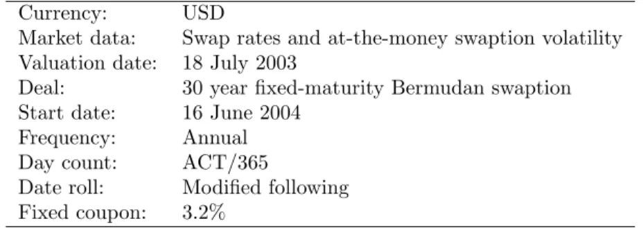
Table 2: Deal description for the test of exact versus approximate drift terms in CMS(q) models.

Currency: USD

Market data: Swap rates and at-the-money swaption volatility Valuation date: 18 July 2003

Deal: 30 year fixed-maturity Bermudan swaption Start date: 16 June 2004

Frequency: Annual

Day count: ACT/365

Date roll: Modified following Fixed coupon: 3.2%

positive. From (16) and Approximation 1, we obtain, dfi:e fi:e ≈ − 1 ˆ pi:e n X k=i+1 ¡_ˆ bk−ˆbe(k) ¢ αk−1 k_Y−2 m=i ¡ 1 +αmfm+1:e(m+1) ¢ σk:e(k)·σi:edt +σi:e·dw(n+1). (24) Define vi= n X k=i+1 ¡_ˆ bk−ˆbe(k) ¢ αk−1 k_Y−2 m=i ¡ 1 +αmfm+1:e(m+1) ¢ σk:e(k). (25)

The proof of the following lemma has been deferred to Appendix B.

Lemma 1 The quantity vi defined in (25) satisfies the following recursive

for-mulas: • vn=0, • vi= ¡ 1 +αifi+1:e(i+1) ¢ vi+1+αi ¡ ˆ_bi+1−ˆ_be(i+1)¢_{σi+1:e(i+1).}

In Algorithm 3 an O(nd) algorithm, based on Lemma 1, has been displayed that approximately calculates the forward swap rates for a time step under the terminal measure, for the CMS(q) market model. This algorithm is exact for the swap market model (q=n).

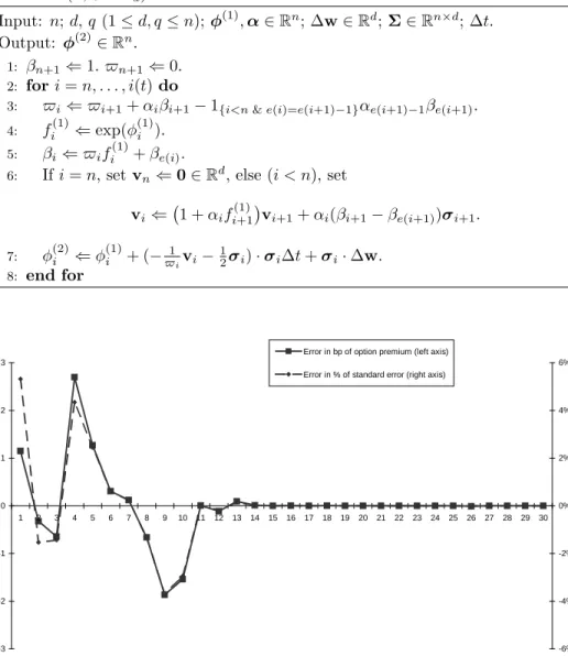
To benchmark the accuracy of Algorithm 3, various fixed-maturity Bermudan swaptions are priced in their corresponding CMS(q) market models, with both exact SDE (16) and approximate SDE (24). The deal specification is given in Table 2. The swap tenor isqyears, with 31−qexercise opportunities, at (16 June 2004 +iyears), i= 0, . . . ,30−q, forq= 1, . . . ,30. The difference between the minimum (0.996) and maximum (1.007) attained day count fractions is 0.011. To price fixed-maturity Bermudan swaptions in Monte Carlo, we use the algorithm of Longstaff & Schwartz (2001), with the swap value as explanatory variable

Algorithm 3 An O(nd)-algorithm for approximately calculating the forward swap rates for a time step in the CMS(q) market model (exact whenq =n), under the terminal measure. The number of factors is denoted by d. The log forward rates, logf(t) = (logfi(t):e(i(t))(t), . . . ,logfn:e(n)(t)) at timet, and

logf(t+ ∆t) at timet+ ∆t, are denoted by φ(1) and φ(2), respectively. Here Σ = (σij) governs the volatility, with σij the time-t volatility of forward rate

fi:e(i)with respect to factorj. Here,e(·) is defined in (2). ∆wshould be sampled

from aN(0,√∆tId) distribution. Input: n;d, q(1≤d, q≤n);φ(1)_,α∈Rn_{; ∆w∈R}d_;Σ∈Rn×d_{; ∆t.} Output: φ(2)∈Rn_. 1: βn+1⇐1. $n+1⇐0. 2: fori=n, . . . , i(t)do 3: $i⇐$i+1+αiβi+1−1{i<n&e(i)=e(i+1)−1}αe(i+1)−1βe(i+1). 4: f_i(1)⇐exp(φ(1)_i ). 5: βi ⇐$ifi(1)+βe(i).

6: Ifi=n, setvn⇐0∈Rd, else (i < n), set

vi ⇐ ¡ 1 +αifi(1)+1 ¢ vi+1+αi(βi+1−βe(i+1))σi+1. 7: φ(2)_i ⇐φ(1)_i + (−_$1 ivi− 1 2σi)·σi∆t+σi·∆w. 8: end for -3 -2 -1 0 1 2 3 1 2 3 4 5 6 7 8 9 10 11 12 13 14 15 16 17 18 19 20 21 22 23 24 25 26 27 28 29 30 q -6% -4% -2% 0% 2% 4% 6% Error in bp of option premium (left axis)

Error in % of standard error (right axis)

Figure 3: Results of the test of exact versus approximate drift terms in CMS(q) models.

x, and basis functions 1, x and x2_{. An 8 factor model is used (d = 8), with}

the correlation of the forward CMS(q) rates given by the parametrization of Rebonato (1998, Equation (4.5), page 83), exp(−β|ti−tj|), for ratesfi:e(i)and

fj:e(j), with β = 3%. The differences between the prices obtained with exact

and approximate drift terms have been displayed in Figure 3. We note that for

q = n, equal prices are obtained up to all digits. The results show that the error is small, up to only 3 bp of the option premium, and up to only 6% of the simulation standard error. Moreover, the error fluctuates robustly around 0, since the differenceαi−αi+q is both negative and positive, in practice.

A significant reduction of computational time can thus be attained by select-ing a low number of factorsd. A result of using a low number of factors is that the instantaneous correlation matrix (ρij) cannot be exactly fit to the

histori-cally estimated or market implied correlation matrix. The procedure for fitting a generic market model to correlation is exactly the same as for the LIBOR market model. For fitting a low-factor LIBOR market model to correlation, the reader is referred to Pietersz & Groenen (2004a,b), Grubiˇsi´c & Pietersz (2005), Wu (2003) and Rebonato (2002, Section 9) or Brigo (2002).

6

Generic Calibration to Correlation

When each particular interest rate derivative has its own generic market model that is used for its valuation and risk management, then the associated input cor-relation to those models involves different interest rates. There is a cor-relationship between these correlations, and this relationship allows for netting correlation risk or reserves. Moreover, utilizing the relationship between the correlations means that correlation is determined consistently across different products. In general all interest rate correlations stem from the correlations between differ-ent segmdiffer-ents of the yield curve. In this section we show how forward LIBOR correlations can be used to determine subsequently the correlations for any of the generic market models specific to certain interest rate products.

The advantage of considering all correlations in this way comes from the fact that one can treat correlation risk (or reserves) in a consistent fashion across all interest rate products. Netting of correlation reserves will subsequently occur naturally. Furthermore only instantaneous forward LIBOR correlations have to be determined and administered.

The key to the method is the well-known fact that, within the LIBOR market model, the instantaneous volatility vector σs:e(t) of a forward swap rate fs:e

can expressed as weighted averages of instantaneous volatility vectors σi(t) of

forward LIBORs, σs:e(t) = e−1 X i=s wis:e(t)σi(t).

An expression for the weightsws:e

i may be found, for example, in Hull & White

(2000, page 53). The weights ws:e

i are state dependent. A highly accurate

be obtained by evaluating the weights at time zero, ˜ σs:e(t) = e−1 X i=s wsi:e(0)σi(t).

From the preceding considerations it should be clear that the instantaneous forward rate correlationρs(1):e(1),s(2):e(2)(t) can be approximately expressed as a

function of the instantaneous forward LIBOR correlationsρij(t),

ρs(1):e(1),s(2):e(2)(t) = ρ ³ _df s(1):e(1)(t) fs(1):e(1)(t) , dfs(2):e(2)(t) fs(2):e(2)(t) ´ = σ T s(1):e(1)(t)σs(2):e(2)(t) q σT s(1):e(1)(t)σs(1):e(1)(t)σTs(2):e(2)(t)σs(2):e(2)(t) , where σT i:j(t)σk:l(t) ≈ σ˜Ti:j(t)σ˜k:l(t) = j−1 X m1=i l−1 X m2=k wi:j m1(0)w k:l m2(0)|σm1(t)||σm2(t)|ρm1m2(t).

7

Conclusions

In this paper, a generalization of market models has been studied, whereby arbitrary forward rates are allowed to span the tenor structure relevant to an in-terest rate derivative. The benefit of such generalization is that straightforward volatility-calibration can be achieved for the fixings of LIBOR or swap rates relevant to the interest rate derivative. Generic market models are therefore particularly apt for pricing and risk management of CMS and hybrid coupon swaps, and callable and cancellable versions thereof, in particular, Bermudan CMS swaptions and fixed-maturity Bermudan swaptions. We showed that the LIBOR and swap market models are special cases of the generic market model framework. The need for a generic specification of market models has been il-lustrated by counting the admissible market model structures withn+ 1 tenor times. We foundn! possible market models. For example, already only for an annual-paying deal of 10 years, there are 10!=3,628,800 market models, thereby establishing the need for a generic specification. Necessary and sufficient con-ditions were derived for a set of forward swap agreements to provide a unique solution for discount bond prices, essentially regardless of the scenario of attained forward rates. The major novelty of this paper is the derivation of generic ex-pressions for no-arbitrage drift terms in generic market models. We developed a novel algorithm of orderO(nd) for approximate drift calculations in CMS market models under the terminal measure.

References

Andersen, L. & Andreasen, J. (2000), ‘Volatility skews and extensions of the LIBOR market model’, Applied Mathematical Finance7(1), 1–32.

Black, F. (1976), ‘The pricing of commodity contracts’, Journal of Financial Economics3(2), 167–179.

Brace, A., G¸atarek, D. & Musiela, M. (1997), ‘The market model of interest rate dynamics’, Mathematical Finance7(2), 127–155.

Brigo, D. (2002), A note on correlation and rank reduction, www. damianobrigo.it.

Cox, J. C. & Ross, S. A. (1976), ‘The valuation of options for alternative stochas-tic processes’,Journal of Financial Economics3(2), 145–166.

Galluccio, S. & Hunter, C. (2004), ‘The co-initial swap market model’,Economic Notes33(2), 209–232.

Galluccio, S., Huang, Z., Ly, J.-M. & Scaillet, O. (2004), Theory and calibration of swap market models, Working Paper, June Version.

Golub, G. H. & van Loan, C. F. (1996), Matrix Computations, 3 edn, John Hopkins University Press, Baltimore, MD.

Grubiˇsi´c, I. & Pietersz, R. (2005), Efficient rank reduction of correlation matri-ces, www.few.eur.nl/few/people/pietersz.

Hull, J. C. & White, A. (2000), ‘Forward rate volatilities, swap rate volatilities, and implementation of the LIBOR market model’,Journal of Fixed Income

10(2), 46–62.

Hunter, C. J., J¨ackel, P. & Joshi, M. S. (2001), ‘Getting the drift’,Risk Magazine. July.

J¨ackel, P. & Rebonato, R. (2003), ‘The link between caplet and swaption volatili-ties in a Brace-G¸atarek-Musiela/Jamshidian framework: approximate solu-tions and empirical evidence’,Journal of Computational Finance6(4), 41– 59.

Jamshidian, F. (1997), ‘LIBOR and swap market models and measures’,Finance and Stochastics1(4), 293–330.

Joshi, M. S. (2003), ‘Rapid computation of drifts in a reduced factor LIBOR market model’, Wilmott Magazine5, 84–85.

Joshi, M. S. & Theis, J. (2002), ‘Bounding Bermudan swaptions in a swap-rate market model’, Quantitative Finance2(5), 370–377.

Longstaff, F. A. & Schwartz, E. S. (2001), ‘Valuing American options by sim-ulation: A simple least-squares approach’, Review of Financial Studies

14(1), 113–147.

Miltersen, K. R., Sandmann, K. & Sondermann, D. (1997), ‘Closed form solu-tions for term structure derivatives with log-normal interest rates’,Journal of Finance 52(1), 409–430.

Musiela, M. & Rutkowski, M. (1997), ‘Continuous-time term structure models: Forward measure approach’,Finance and Stochastics1(4), 261–291. Ostrom, D. (1998), ‘Japanese interest rates enter negative territory’,Japan

Eco-nomic Institute Report(43B), 4–6. www.jei.org/archive/.

Pietersz, R. & Groenen, P. J. F. (2004a), ‘A major LIBOR fit’,Risk Magazine

p. 102. December.

Pietersz, R. & Groenen, P. J. F. (2004b), ‘Rank reduction of correlation matrices by majorization’,Quantitative Finance.

Pietersz, R. & Pelsser, A. A. J. (2004), ‘Risk-managing Bermudan swaptions in a LIBOR model’,Journal of Derivatives11(3), 51–62.

Pietersz, R., Pelsser, A. A. J. & van Regenmortel, M. (2004a), ‘Bridging brow-nian LIBOR’, Wilmott Magazine. Forthcoming.

Pietersz, R., Pelsser, A. A. J. & van Regenmortel, M. (2004b), ‘Fast drift-approximated pricing in the BGM model’, Journal of Computational Fi-nance 8(1), 93–124.

Rebonato, R. (1998), Interest Rate Option Models, 2 edn, J. Wiley & Sons, Chichester.

Rebonato, R. (2002), Modern Pricing of Interest-Rate Derivatives, Princeton University Press, New Jersey.

Rebonato, R. (2004), ‘Interest-rate term-structure pricing models: a review’,

Proceedings of the Royal Society London460, 667–728. Series A.

Rubinstein, M. (1983), ‘Displaced diffusion option pricing’,Journal of Finance

38(1), 213–217.

Schl¨ogl, E. (2002), ‘A multicurrency extension of the lognormal interest rate market models’,Finance and Stochastics 6(2), 173–196.

Wu, L. (2003), ‘Fast at-the-money calibration of the LIBOR market model using Lagrange multipliers’,Journal of Computational Finance6(2), 39–77.