Microaneurysm Detection using Fully Convolutional
Neural Networks
Piotr Chudzika,∗, Somshubra Majumdarb, Francesco Caliv´aa, Bashir Al-Diria, Andrew Huntera
aSchool of Computer Science, University of Lincoln, LN6 7TS, Lincoln, UK. bDepartment of Computer Science, University of Illinois, IL 60607, Chicago, USA.
Abstract
Backround and Objectives: Diabetic retinopathy is a microvascular
complica-tion of diabetes that can lead to sight loss if treated not early enough. Mi-croaneurysms are the earliest clinical signs of diabetic retinopathy. This paper
presents an automatic method for detecting microaneurysms in fundus
pho-tographies.
Methods: A novel patch-based fully convolutional neural network with batch
normalization layers and Dice loss function is proposed. Compared to other
methods that require up to five processing stages, it requires only three.
Fur-thermore, to the best of the authors’ knowledge, this is the first paper that shows
how to successfully transfer knowledge between datasets in the microaneurysm
detection domain.
Results: The proposed method was evaluated using three publicly available and widely used datasets: E-Ophtha, DIARETDB1, and ROC. It achieved
bet-ter results than state-of-the-art methods using the FROC metric. The proposed
algorithm accomplished highest sensitivities for low false positive rates, which
is particularly important for screening purposes.
Conclusions: Performance, simplicity, and robustness of the proposed method
demonstrates its suitability for diabetic retinopathy screening applications.
Keywords: Medical Image Analysis, Microaneurysm Detection,
∗Corresponding author
Convolutional Neural Networks, Retinal Fundus Images
1. Introduction
Diabetes affects one in eleven adults (over 400 million people worldwide) [1].
Diabetic retinopathy (DR) is a microvascular complication of diabetes which
is the leading cause of vision loss in the working-age population [2]. One out
of three diabetics has DR [3] and one in ten diabetic patients develops most 5
vision-threatening form of DR [4]. Early detection of DR can prevent blindness
in 90% of cases [5].
DR screening is manually performed by ophthalmologists and trained graders
through a visual inspection of fundus photographs (FP). Unfortunately, the grading process is time-consuming, tedious, and error-prone with high inter-10
observer variability. Due to the rising number of DR patients worldwide
(ex-pected to exceed 640m by 2040 [1]) and their location (75% live in
underdevel-oped areas [6]) the development of computer-assisted diagnosis and automatic
DR screening approaches are of the utmost importance.
Microaneurysms (MAs) are spherical swellings of the capillaries caused by 15
weakening of the vascular walls; they appear as small round red dots. They
are the earliest clinical sign of DR and continue to be present as the disease
progresses. Consequently, automated detection of MAs can drastically reduce
the screening workload. MA detection is a challenging task even for the human eye due to many factors including uneven image illumination, reflections, limited 20
resolution and media opacity. The boundaries of MAs are not always
well-defined and local contrast to the background is low, even in high-resolution
images. Moreover, MAs may be confounded with visually similar anatomical
structures such as haemorrhages, junctions in thin vessels, disconnected vessel
segments, dark patches on vessels, background pigmentation patches and dust 25
particles on the camera lense.
In general, the majority of MA detection methods consists of up to five
Can-didate feature extraction, and 5) Classification. The main goal of preprocessing
is to remove noise, correct non-uniform illumination, and to improve contrast 30
between the MAs and background. The MA candidate extraction stage uses a simple algorithm to identify a reasonably small set of locations with somewhat
“lesion-like” appearance, attempting to identify all actual lesions together with
many false positive regions. The vessel removal stage addresses the large number
of false positives that may otherwise be produced by vessels. Next, hand-crafted 35
features are extracted from candidate regions; this is the most labour-intensive
and time-consuming part of the design stage. Finally, a classifier is trained to
distinguish MAs from non-MAs based on the extracted features.
Baudoinet al.[7] introduced the first MA detection algorithm applied to
flu-orescein angiogram images. They employed a mathematical morphology based 40
approach to remove vessels and applied a top-hat transformation with linear structuring elements to detect MAs. Several methods were built on this
ap-proach [8], however, since intravenous use of fluorescein can cause death in 1 in
222 000 cases [9], such methods are not suited for screening purposes. Walteret
al.[10] also used a top-hat based method and automated thresholding to extract 45
MA candidates. They extracted 15 features and applied kernel density
estima-tion with variable bandwith for MA classificaestima-tion. In general, morphology-based
approaches are sensitive to changes in size and shape of structuring elements
which result in significant variations in MAs detection results. Zhanget al.[11]
proposed a method based on dynamic thresholding and correlation coefficients 50
of a multi-scale Gaussian template. They used 31 manually designed features based on intensity, shape and response of a Gaussian filter. Veiga et al. [12]
presented an algorithm using Law texture features. Support Vector Machines
(SVM) were used in a cascading manner: first SVM was used to extract MA
can-didates whereas the second SVM performed final MA classification. Haloi [13] 55
used a vanilla convolutional network with 3 convolutional layers and 2 fully
connected layers to detect MAs. Javidi et al. [8] proposed a technique which
used 2D Morlet wavelet to find MA candidates. At the next stage, a
structures. Srivastavaet al. [14] used Frangi-based filters that were manually 60
designed to distinguish vessels from red lesions. Filters were applied to multiple
sized image patches to extract features. Finally, these features were classified using a SVM.
Compared to the methods mentioned above, the proposed algorithm requires
only three stages instead of five (preprocessing, patch extraction and classifica-65
tion). There is no need for MA candidate detection, vessel removal or feature
extraction. Furthermore, the proposed method does not require manually
hand-crafted features, it automatically learns the most discriminative features for MA
detection. The vast majority of MA detection algorithms employ features based
on MA shape, colour and texture. Unfortunately, many image modalities makes 70
it virtually impossible to model them manually. To address this challenge, a
Convolutional Neural Network (CNN) was used. CNNs have emerged as a powerful family of algorithms for solving computer vision tasks such as object
detection [15], semantic segmentation [16] and image classification [17].
Com-pared with [13] method, the presented algorithm proposes a novel fully convo-75
lutional neural network (FCNN) architecture and transfers knowledge between
MA datasets.
Training CNNs from scratch is not a trivial task, as they require large
amounts of labelled data for training. In the MA detection domain, public
datasets are small, scarce, and local lesion annotations on a per-pixel level are 80
almost non-existent (to the best of authors knowledge, only one such dataset
exists [18]). Moreover, the CNNs have vast capacity as learning models with millions of learnable parameters. As a result, they are very prone to overfitting
and various convergence difficulties. Consequently, the initial values of a
net-work’s weights have paramount importance in the learning process, especially 85
for avoidance of local minima and saddle points.
To address these challenges, prior knowledge in the form of a network’s
weights can be transferred between models that are later fine-tuned with new
data. Azizpouret al.[19] showed that the success of knowledge transfer depends
on the similarity between the training dataset of a CNN, and the dataset to 90
which the knowledge is transferred. Given the limited availability of large
medi-cal datasets, research on transfer learning in medimedi-cal imaging is largely focussed
on transferring knowledge from general natural images datasets. However, these datasets have very different properties to medical datasets, including the fact
that in medical datasets objects of interest may be very small and boundaries 95
are of paramount importance. Consequently, knowledge transfer between these
two domains is not optimal and produces various success rates [19]. In this
pa-per we show that knowledge transfer even between small medical datasets can
produce state-of-the-art results with an appropriate network architecture. To
the best of our knowledge, this is the first time that deep transfer learning has 100
been applied in the MA detection domain.
The main contributions of this paper are as follows. First, we propose a
MA detection method that requires only three stages of analysis. Second, we present a novel CNN with a dedicated architecture for MA detection that does
not require hand-crafted features. Third, we show how to successfully transfer 105
knowledge between small datasets in MA domain - an important innovation in
this domain as retinal image set characteristics vary between cameras, so that
any practically useful method must be capable of simple and reliable retraining.
This paper is organized as follows. The proposed method is described in
Section II. Section III describes the datasets and performance metrics used for 110
experiments. In Section IV the evaluation results are presented and compared
with existing approaches. Finally, in Section V discussion and conclusions are
given.
2. Proposed Method
Fig. 1 shows a general overview of the proposed method. It consists of three 115
main stages: preprocessing, patch extraction and pixel-wise classification. The
main objective of the preprocessing stage is to remove the non-uniform illumi-nation and redundant data from images. The patch extraction stage prepares
with a novel architecture. 120
2.1. Preprocessing
First, we extract the green plane of the fundus image as it provides the highest contrast between foreground structures, such as lesions and vessels, and
the background. Since we are only interested in pixels inside a Field-of-View
(FOV), we automatically generate a mask for pixels outside the FOV. A mask 125
is generated by applying Otsu thresholding [20] to the green plane of the
im-age. Noisy regions are removed by morphological opening and closing with a
structuring element of size five. Next, the image is cropped to the size defined
by its FOV to accelerate further processing. Subsequently, the image is resized
to the smallest image width of the E-ophtha dataset [18], while maintaining the 130
aspect ratio, using bicubic interpolation. Simultaneously, the same operations are applied to the corresponding annotation image. Finally, each image (I) was
preprocessed (Ip) by computing a weighted sum as in Eq. 1:
Ip=I·α+IGauss·β+γ (1)
where alpha= 4 and β =−10 are weight factors; IGauss is Gaussian blurred
image that was created using filter computed as described in Eq. 2 withσ= 10; 135
γ= 128 is a scalar added to each sum.
G(x, y) = 1 2πσ2e
−x2 +y2
2σ2 (2)
All values were determined experimentally. Fig. 3 shows an example
prepro-cessed image.
2.2. Pixel-Wise Classification
The main goal of this stage is to classify each pixel as either MA or non-140
MA. We cast pixel-wise classification as a probabilistic classification task, where
each pixel can be assigned a continuous value between 0 (non-MA) and 1 (MA).
Compared to other works which perform a binary classification, this learning
task is more challenging because the expected output is more complex, hence
the underlying data distribution function is harder to model. 145
The CNN is trained to map an image patchP to the corresponding
annota-tionA(P) for all possible locations within an image. A training sample consists
ofS×S sizedP andA(P) : {P, A(P)}.
The goal of training is to learn a mappingP →A(P) in the form of a CNN by minimizing 150 L= N X i=1 l(A(P)i, f(Pi; Θ)) + Φ(Θ)), (3)
where A(P)i and Pi are the i-th annotation patch and i-th image patch,
N is the number of training samples, l(·) is the loss function, Θ are learning parameters, and Φ(Θ) is the regularization term.
2.2.1. Patch Generation
At training time, all possible image patches are extracted from each training 155
image using a sliding window approach with 2×2 stride. The patches are divided into two groups: MA patches containing at least 1 MA pixel and
non-MA patches consisting of all remaining patches. Both non-MA and non-non-MA patches
are randomly sampled from the set of all possible patches. Patches that are completely outside the FOV are discarded. Each training sample is subject 160
to random artificial transformations (AT) including rotation, horizontal and
vertical reflections with 0.5 probability. The ATs are performed to increase
variety in the training set and combat overfitting; they are performed during
CNN training so their computational footprint is limited. The proposed method
works on a pixel level hence even MA patches consist of more non-MA pixels 165
than MA pixels. As such, MA patches provide both positive and negative
training samples. Nevertheless, we added a small set of non-MA patches to the
training set to provide network with examples of as many as possible retinal structures(e.g. fovea, optic nerve head) and backgrounds. As a result, the
training set consists in 80% of MA patches and in 20% of non-MA patches. 170
At testing time, all possible image patches from inside of a FOV are
used. EachA(P) produced by the model provides a single vote for all pixels it
contains. Given that patches are centred at all possible locations and theA(P)
size isS×S, each pixel receives S2 votes, and a pixel receiving v votes as an 175
MA is assigned a probability of v/S2. As a result, a confidence map for pixel
MA membership is created.
2.2.2. CNN Architecture and Training
Inspired by [21], we adopted a fully convolutional approach when designing the CNN. The architecture of the CNN is similar to a convolutional autoencoder: 180
it consists of “contracting” and “expanding” paths. The “contracting” path is
used to extract most discriminative features from input (encode the input),
whereas the “expanding” path is tasked with recreating and classifiying the
input by using upscaling and 1×1 convolution operations. Skip connections between the two paths allow for a direct flow of feature maps from earlier to 185
latter layers, which is beneficial for the learning process [22]. Ronnenberg et
al. [21] designed their fully convolutional neural networks for segmentation of
whole images in one pass. As MAs are local features, it is more appropriate
here to use a network with a small receptive field and a sliding window approach to processing. Compared with [21], the proposed architecture works on small 190
image patches, incorporates batch normalization (BN) layers and uses different
loss function. As MAs occupy a very small proportion of fundus images that
feature them, there is a significant class imbalance in the problem domain. To
address this we incorporated a Dice coefficient function [23] as a loss function
as it effectively handles the overwhelming number of true negatives. The Dice 195
coefficient loss function was used before with CNNs [22] but not in context of
MA detection. The training algorithm maximises the Dice loss function which
measures the overlap between ground truthsyand predicted segmentation ˆy. Its
values range between 0 (no overlap) and 1 (perfect agreement) and is calculated as
200
DICE =2∗ |y
Tyˆ|+δ
whereδis a small smoothing factor that counteracts against zero value and
zero denominator.
The MA detection domain suffers from a common problem in medical imag-ing that stems from data scarcity, known as Covariate Shift: the distribution
of features is different for subsets of training and test datasets which violates 205
the i.i.d.(independent and identically distributed) assumption of many machine
learning (ML) algorithms [24]. This may result from the use of different retinal
camera systems and/or camera settings. The Covariate Shift in small datasets
renders the modelling of true data distribution using ML models virtually
im-possible. To mitigate this difficulty and make data comparable across features, 210
a normalization technique (shifting data to zero mean and unit variance) is
used as a preprocessing step [24]. The same phenomenon occurs during training
deep CNNs which are hierarchical in nature and is called Internal Covariate Shift [25]. A small change in lower layers can cause a landslide effect in
up-per layers due to changes in the distribution of upup-per layer inputs. Ioffe and 215
Szegedy [25] proposed a batch normalization layer that partially alleviates the
Internal Covariate Shift by normalizing/whitening data flowing between layers.
The use of BN layers in CNNs results in faster convergence (higher learning
rates) and better regularization (by constraining layer’s inputs, it’s weights are
also indirectly constrained). 220
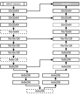
The CNN architecture was determined experimentally and is depicted in
Fig. 2. It consists of 18 convolutional layers, each followed by a BN layer apart
from the final classification layer; three 2×2 max-pooling layers in the “contrac-tive” path and corresponding three 2×2 simple upsampling layers that replicate rows and columns of data in the “expanding” path; 4 skip connections between 225
both paths. Double inputs in the “expanding” path are merged by
concatena-tion. All convolutional layers use 3×3 filters and ReLU activation function [26] apart from the final layer which uses a sigmoid activation function. Weights
are updated using stochastic gradient descent with batch size 128 and Adam
optimization technique [27] with 0.0001 initial learning rate. All training pairs 230
Fine-tuning is a process of training a neural network from a set of
pre-defined weights [28]. A traditional approach to fine-tine deep neural networks
(DNN) is to train only the final layers of a network using a small learning rate. Similarly to [28], it was observed that such approach can provide sub-235
optimal performance. To find the best ratio between trained and frozen layers,
an iterative approach with varying train/freeze ratio was employed on a small
dataset.
3. Materials and Evaluation
The proposed algorithm was evaluated using most widely used performance 240
metrics and publicly available datasets which are described below.
3.1. Datasets
E-Ophthadataset [18] consists of 381 compressed images of which 148 have
MAs presents and 233 depict healthy FPs. Images were acquired at more than
30 screening centres around France at various resolutions at 45◦ FOV. There 245
are no separate testing and training datasets provided. The variety of image
quality, resolution and illumination conditions makes it the most challenging
publicly available dataset. To the best of the authors’ knowledge, this is the
only public dataset that provides pixel-wise ground truths of MAs.
ROCdataset [29] is composed of 50 training and 50 test compressed images. 250
Images were captured by three different fundus cameras at various resolutions
ranging from 768×576 to 1389×1383 at 45◦FOV. All images were annotated by four experienced graders. Since test ground truths were never made public
and the ROC competition website is inactive [29], only training ground truths
are available. 37 images of the training set have at least one MA present, and 255
remaining 13 images present healthy FPs.
DIARETDB1 dataset [30] comprises of 28 training and 61 test
uncom-pressed images acquired at 50◦ FOV. Each 1500×1152 image was manually annotated for presence of MAs and HEs by four medical experts. The final
ground truths were created by fusing all annotations with 75% confidence. 38 260
FPs have no MAs present whereas remaining 51 FPs have at least one MA.
Since the E-Ophtha dataset does not provide separate train and test sets, it is randomly divided into two sets containing 190 and 191 images respectively.
During experimentation 2-fold cross-validation is performed, with each subset
alternatively treated as the training or testing set. A similar approach is used 265
with the ROC training dataset, which is split into two sets of 25 images each.
DI-ARETDB1 is explicitly divided into training and testing datasets and we utilise
the standard split during experiments. ROC and DIARETDB1 datasets do not
provide pixel-wise ground truths however they offer central points and radii of
all MAs. Following common practice, we use this information to calculate eval-270
uation metrics. All datasets have been acquired using similar FOV(either 45◦ or 50◦). As a result, the downsampling process produces lesions with a common scale. It is important to note that when dealing with images acquired using very
different FOVs, the downsampling alone is not enough to successfully normalize
lesions and other techniques are necessary (e.g. FOV cropping). 275
3.2. Evaluation Metrics
The free-response ROC (FROC) curve is the most commonly used metric for
abnormality detection in medical imaging. It plots per-lesion sensitivity against
the average number of false positives per image for different threshold values.
In contrast to ROC or specificity-based measures, FROC provides meaningful 280
statistics despite the class imbalance between non-MA and MA pixels in an
image. Following common practice we calculate a sensitivity score at seven
average false positives per image (FPI) points: 1/8,1/4,1/2,1,2,4,8 [29].
Fol-lowing common practice, we define lesion as a true positive if at least one pixel
overlaps with a corresponding ground truth lesion [12]. We performed Wilcoxon 285
signed ranked tests to estimate the statistical significance of results. Tests were conducted using 255 sensitivity values corresponding to all possible greyscale
4. Experimental Results
To assess the performance of the proposed method we performed two sets 290
of experiments. In the first set of experiments we evaluate and compare
fine-tuning schemes. In the second, we compare the performance of proposed MA
detection technique with other state-of-the-art methods.
The implementation was based on Keras deep learning framework [31] and
Tensorflow numerical computation library [32]. The experiments were con-295
ducted using a PC with Intel Core i7-6700K CPU, two NVIDIA TitanX graphics cards, and 64GB of RAM.
4.1. Model Description
Table 1: Training data.
Dataset Nr of training images Nr training patches
ROC 50 72 481
DIARETDB1 28 40 549
E-Ophtha 381 552 451
Table 1 shows the amount of training images and patches used for
experi-ments. 10% of the training samples are held back as a validation set and an 300
early stopping criteria is used: training stops when validation error does not
im-prove for 20 epochs. If the validation error does not imim-prove for 10 epochs, the learning rate is reduced by a factor of 0.3. During testing all possible patches
are extracted from the FOV and forward propagated through the network. All
experiments apart from the E-Ophtha evaluation use a network trained on 354 305
randomly selected E-Ophtha images, and evaluated on remaining 27 images, as
the base model. All parameters were determined empirically based on authors
experience or successful deep learning works ( [15], [16], [21]). We observe that
the proposed approach is robust to changes in parameters’ values. The
modifi-cation of parameters barely affects the final results, however it has a moderate 310
impact on speed of error convergence. We conclude that the system is not
sen-sitive to small parameters change, however such changes can affect the amount
of time needed for training.
4.2. Fine-Tuning
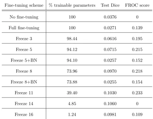
Table 2: Comparison od fine-tuning schemes.
Fine-tuning scheme % trainable parameters Test Dice FROC score
No fine-tuning 100 0.0376 0 Full fine-tuning 100 0.0271 0.139 Freeze 3 98.44 0.0616 0.195 Freeze 5 94.12 0.0715 0.215 Freeze 5+BN 94.10 0.0257 0.152 Freeze 8 73.96 0.0970 0.218 Freeze 8+BN 73.88 0.0255 0.154 Freeze 11 39.40 0.1030 0.233 Freeze 14 4.85 0.1060 0 Freeze 16 1.24 0.0981 0.109
To find the optimal fine-tuning scheme we performed 10 experiments using 315
ROC training dataset; we randomly divided this into a 25 image training set
and 25 image test set, using the same split for all experiments. The base model
for fine-tuning was trained on the E-Ophtha dataset as described above. Unless
stated otherwise, during fine-tuning the same early stopping and training
hyper-parameters were used as in the case of base model training. 320
Table 2 shows a comparison of all fine-tuning schemes. The Dice metric was
calculated on per-pixel basis for the test dataset. In our experiments we
layers as proposed by [28]. As expected, networks trained from scratch (no
fine-tuning) and fully retrained (full fine-fine-tuning) provided the worst results. The 325
network without any fine-tuning did not produce a FROC score because the lowest achieved FPI was just below 0.5, and to calculate the FROC score all
seven FROC values are required. For comparison purposes we assign a 0 value
to all methods that fail to produce the FROC score. These approaches do not
take full advantage of already provided knowledge in the form of a base model. 330
Freezing BN layers results in worse performance compared with the same models
when BN layers are trainable. The network with 14 initial layers frozen achieved
a comparably high test DICE, which means that it still produced competitive
results for all possible pixels. However, the per-lesion evaluation showed that
the lowest FPI it managed to reach was around 0.25 which is not enough to cal-335
culate a FROC score. As expected, freezing the final most task-specific layers results in decreased performance. We observe that by increasing the number of
frozen initial layers, our model accomplishes the best performance by freezing
11 initial layers and training 7 final layers. As a result, all following experiments
will use this fine-tuning scheme when transferring knowledge between datasets. 340
4.3. Microaneurysm detection
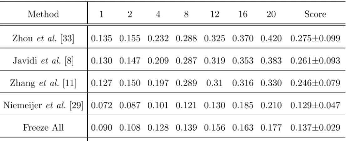
Table 3: The sensitivies at various FPIs using ROC training dataset.
Method 1 2 4 8 12 16 20 Score Zhou et al.[33] 0.135 0.155 0.232 0.288 0.325 0.370 0.420 0.275±0.099 Javidiet al.[8] 0.130 0.147 0.209 0.287 0.319 0.353 0.383 0.261±0.093 Zhanget al.[11] 0.127 0.150 0.197 0.289 0.31 0.316 0.330 0.246±0.079 Niemeijeret al.[29] 0.072 0.087 0.101 0.121 0.130 0.185 0.210 0.129±0.047 Freeze All 0.090 0.108 0.128 0.139 0.156 0.163 0.177 0.137±0.029 Proposed Method 0.174 0.243 0.306 0.385 0.431 0.461 0.485 0.355±0.109
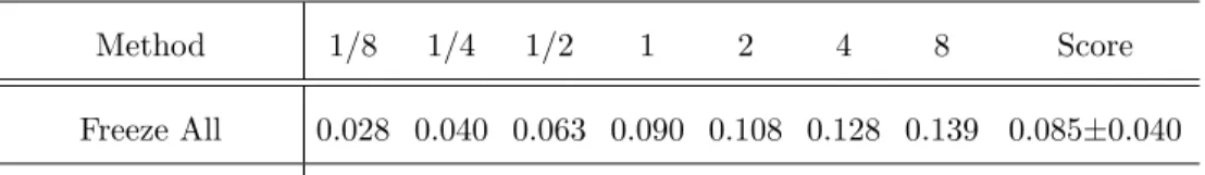
Table 4: The sensitivies at low FPIs using ROC training dataset.
Method 1/8 1/4 1/2 1 2 4 8 Score
Freeze All 0.028 0.040 0.063 0.090 0.108 0.128 0.139 0.085±0.040
Proposed Method 0.039 0.067 0.141 0.174 0.243 0.306 0.385 0.193±0.116
Table 3 presents a performance comparison between the proposed method
and state-of-the-art methods using the ROC training dataset. The Freeze All
method corresponds to a FCNN without any fine-tuning. Compared to other
techniques, the proposed algorithm achieves the highest average FROC score of 345
0.355. Most importantly, it provides much better performance for low FPIs. For comparison purposes, we present the sensitivites at seven high FPIs.
Nonethe-less, similarly to [29] we think that sensitivity values at FPI higher than 1.08 are
of little clinical importance. Consequently, we provide the performance metrics
for much lower FPI in Table 4. 350
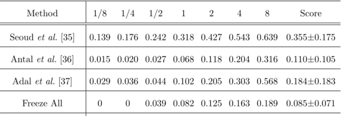
Table 5 shows a comparison of MA detection methods using the DIARETDB1
dataset. Consistently with ROC results, the proposed algorithm produces the
highest average score of 0.392. Furthermore, the sensitivities for all FPIs are
higher than provided by other methods. To transfer knowledge from the base
model to models used with ROC and DIARETDB1 datasets, 11 initial layers 355
of the base model were frozen with remaining 7 trained with new data. Table 6 presents the performance comparison using E-Ophtha dataset. This dataset is
much bigger than the previous datasets which results in bigger training datasets.
The DNNs benefit from bigger datasets [34] hence the results are better than
compared with other datasets. Fig. 4 presents FROC curves produced by the 360
proposed algorithm for all three datasets.
Table 7 shows results of Wilcoxon signed rank tests between the proposed
method and Freeze All method for ROC and DIARETDB1 datasets. The null
hypothesis is that the proposed method provides similar results to Freeze All
method, whereas the alternative hypothesis is that the proposed method pro-365
vides better results than Freeze All method. In our case, the null and alternative
hypotheses can be defined asH0 :MP =MF and H1 :MP > MF, where MP
and MF are medians of sensitivity values produced by the proposed method
and Freeze All method respectively. Following common practice, we set the
significance level at 0.05. Wilcoxon signed rank tests show statistically signifi-370
cant improvement in the sensitivity values when using the proposed approach
(p0.05).
Table 5: The sensitivies at various FPIs using DIARETDB1 dataset.
Method 1/8 1/4 1/2 1 2 4 8 Score Seoudet al. [35] 0.139 0.176 0.242 0.318 0.427 0.543 0.639 0.355±0.175 Antalet al.[36] 0.015 0.020 0.027 0.068 0.118 0.204 0.316 0.110±0.105 Adalet al. [37] 0.029 0.036 0.044 0.102 0.205 0.303 0.568 0.184±0.183 Freeze All 0 0 0.039 0.082 0.125 0.163 0.189 0.085±0.071 Proposed Method 0.187 0.246 0.288 0.365 0.449 0.570 0.641 0.392±0.157
Table 6: The sensitivies at various FPIs using E-ophtha dataset.
Method 1/8 1/4 1/2 1 2 4 8 Score
Veigaet al.[12] 0.110 0.152 0.222 0.307 0.383 0.494 0.629 0.328±0.174
Proposed Method 0.185 0.313 0.465 0.604 0.716 0.801 0.849 0.562±0.233
Table 7: Wilcoxon signed rank test results. Sincep0.05, results are statistically significant.
Compared Methods p-value
ROC: Proposed method vs Freeze All 1.97×10−43
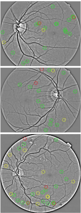
Fig. 6 presents examples of lesion detection results. The detection results
were calculated at 1.08 FPI rate which is regarded as clinically acceptable [29].
We observe that many false positive detections are difficult to discern even for a 375
human eye. Similarly to [30] we observe high inter-observer variability between
human graders, which negatively affects the quality of provided ground truths
and trained models.
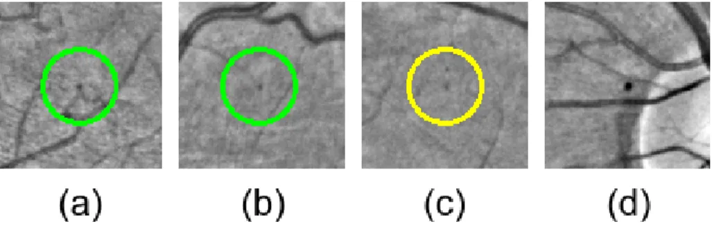
Fig. 5 shows examples of various challenging detections. Many detection
al-gorithms have to extract and remove vessels first to correctly detect MAs close 380
to vessels. Fig. 5 (a) shows that the proposed method can successfully detect
MAs very close to vessels. In fig. 5 (b) the MA is almost at the end of a small
vessel. Fig. 5 (c) presents a false positive example, which is a subtle
pigmenta-tion change. DIARETDB1 dataset contains dust artefacts located in exactly the
same location across many images. Fig. 5 (d) shows that the proposed method 385
correctly ignores such artefact.
5. Discussion
The proposed algorithm achieves better results than state-of-the-art methods
in terms of the FROC metric. Most importantly, it provides highest performance at low FPIs which are particularly significant for screening application. An MA 390
detection system for screening purposes does not have to find all MAs, but
enough MAs to help a clinician decide if a patient needs referral. As such, we
think that the proposed algorithm would prove useful as a component of a DR
screening process.
The total time required to process a single image is around 220 seconds. 395
The majority of this time is spent on forward propagating the large amount of
patches through the network. However, during this study we did not concentrate
on algorithm’s efficiency, hence the implementation is experimental and can be
improved. The processing time per image could be drastically reduced if the forward propagation step would be parallelized across multiple devices. This 400
used devices.
6. Conclusions
This paper presents a novel MA detection method evaluated using three
publicly available datasets. The proposed algorithm uses a novel FCNN archi-405
tecture with BN layers and Dice coefficient loss function to segment and detect
MAs. Compared to other techniques that typically require five computational
stages, the proposed method requires only three. Furthermore, we show how
to successfully and efficiently transfer knowledge between small datasets in the
MA detection domain. 410
Almost all current MA detection methods rely on human-crafted features,
hence their usability and robustness is dependent on the designer’s knowledge,
experience, and skills. Such systems have to be manually recalibrated due to
ever-changing image modalities. The proposed method extracts the most
dis-criminative features for MA detection automatically and proves to be robust 415
against changes in image illumination or contrast. In the future, we are
plan-ning to parallelize the inference step and reduce the processing time to the range
of seconds.
Acknowledgments
This research was made possible by a Marie Curie grant from the Euro-420
pean Commission in the framework of the REVAMMAD ITN (Initial Training
Research network), Project number 316990.
Conflict of interest statement
No potential conflict of interest was reported by the authors.
References
425
[1] Idf diabetes atlas, 7th edn., International Diabetes Federation.
[2] N. Cheung, P. Mitchell, T. Wong, Diabetic retinopathy, Lancet 376 (9735)
(2010) 124–36.
[3] J. Ding, T. Y. Wong, Current epidemiology of diabetic retinopathy and 430
diabetic macular edema, Current diabetes reports 12 (4) (2012) 346–354.
[4] J. W. Yau, S. L. Rogers, R. Kawasaki, E. L. Lamoureux, J. W. Kowalski, T. Bek, S.-J. Chen, J. M. Dekker, A. Fletcher, J. Grauslund, et al., Global
prevalence and major risk factors of diabetic retinopathy, Diabetes care
35 (3) (2012) 556–564. 435
[5] R. J. Tapp, J. E. Shaw, C. A. Harper, M. P. De Courten, B. Balkau, D. J.
McCarty, H. R. Taylor, T. A. Welborn, P. Z. Zimmet, The prevalence of and
factors associated with diabetic retinopathy in the australian population,
Diabetes care 26 (6) (2003) 1731–1737.
[6] L. Guariguata, D. Whiting, I. Hambleton, J. Beagley, U. Linnenkamp, 440
J. Shaw, Global estimates of diabetes prevalence for 2013 and projections
for 2035, Diabetes research and clinical practice 103 (2) (2014) 137–149.
[7] C. Baudoin, B. Lay, J. Klein, Automatic detection of microaneurysms in
di-abetic fluorescein angiography., Revue d’´epid´emiologie et de sant´e publique 32 (3-4) (1983) 254–261.
445
[8] M. Javidi, H.-R. Pourreza, A. Harati, Vessel segmentation and
microa-neurysm detection using discriminative dictionary learning and sparse
rep-resentation, Computer Methods and Programs in Biomedicine 139 (2017)
93–108.
[9] L. A. Yannuzzi, K. T. Rohrer, L. J. Tindel, R. S. Sobel, M. A. Costanza, 450
W. Shields, E. Zang, Fluorescein angiography complication survey,
Oph-thalmology 93 (5) (1986) 611–617.
[10] T. Walter, P. Massin, A. Erginay, R. Ordonez, C. Jeulin, J.-C. Klein,
Auto-matic detection of microaneurysms in color fundus images, Medical image
analysis 11 (6) (2007) 555–566. 455
[11] B. Zhang, X. Wu, J. You, Q. Li, F. Karray, Detection of microaneurysms
using multi-scale correlation coefficients, Pattern Recognition 43 (6) (2010)
2237–2248.
[12] D. Veiga, N. Martins, M. Ferreira, J. Monteiro, Automatic microaneurysm detection using laws texture masks and support vector machines, Com-460
puter Methods in Biomechanics and Biomedical Engineering: Imaging &
Visualization (2017) 1–12.
[13] M. Haloi, Improved microaneurysm detection using deep neural networks,
arXiv preprint arXiv:1505.04424.
[14] R. Srivastava, L. Duan, D. W. Wong, J. Liu, T. Y. Wong, Detecting retinal 465
microaneurysms and hemorrhages with robustness to the presence of blood
vessels, Computer Methods and Programs in Biomedicine 138 (2017) 83–91.
[15] K. Simonyan, A. Zisserman, Very deep convolutional networks for
large-scale image recognition, arXiv preprint arXiv:1409.1556.
[16] J. Long, E. Shelhamer, T. Darrell, Fully convolutional networks for seman-470
tic segmentation, in: Proceedings of the IEEE Conference on Computer
Vision and Pattern Recognition, 2015, pp. 3431–3440.
[17] A. Krizhevsky, I. Sutskever, G. E. Hinton, Imagenet classification with deep convolutional neural networks, in: Advances in neural information
processing systems, 2012, pp. 1097–1105. 475
[18] E. Decenci`ere, G. Cazuguel, X. Zhang, G. Thibault, J.-C. Klein, F. Meyer,
B. Marcotegui, G. Quellec, M. Lamard, R. Danno, et al., Teleophta:
Ma-chine learning and image processing methods for teleophthalmology, IRBM
34 (2) (2013) 196–203.
[19] H. Azizpour, A. Sharif Razavian, J. Sullivan, A. Maki, S. Carlsson, From 480
generic to specific deep representations for visual recognition, in:
Proceed-ings of the IEEE Conference on Computer Vision and Pattern Recognition
[20] N. Otsu, A threshold selection method from gray-level histograms, IEEE
transactions on systems, man, and cybernetics 9 (1) (1979) 62–66. 485
[21] O. Ronneberger, P. Fischer, T. Brox, U-net: Convolutional networks for biomedical image segmentation, in: International Conference on Medical
Image Computing and Computer-Assisted Intervention, Springer, 2015, pp.
234–241.
[22] M. Drozdzal, E. Vorontsov, G. Chartrand, S. Kadoury, C. Pal, The im-490
portance of skip connections in biomedical image segmentation, in:
In-ternational Workshop on Large-Scale Annotation of Biomedical Data and
Expert Label Synthesis, Springer, 2016, pp. 179–187.
[23] L. R. Dice, Measures of the amount of ecologic association between species,
Ecology 26 (3) (1945) 297–302. 495
[24] J. Quionero-Candela, M. Sugiyama, A. Schwaighofer, N. D. Lawrence,
Dataset shift in machine learning, The MIT Press, 2009.
[25] S. Ioffe, C. Szegedy, Batch normalization: Accelerating deep network
train-ing by reductrain-ing internal covariate shift, arXiv preprint arXiv:1502.03167.
[26] G. E. Dahl, T. N. Sainath, G. E. Hinton, Improving deep neural networks 500
for lvcsr using rectified linear units and dropout, in: Acoustics, Speech
and Signal Processing (ICASSP), 2013 IEEE International Conference on,
IEEE, 2013, pp. 8609–8613.
[27] D. Kingma, J. Ba, Adam: A method for stochastic optimization, arXiv
preprint arXiv:1412.6980. 505
[28] N. Tajbakhsh, J. Y. Shin, S. R. Gurudu, R. T. Hurst, C. B. Kendall, M. B.
Gotway, J. Liang, Convolutional neural networks for medical image
anal-ysis: full training or fine tuning?, IEEE transactions on medical imaging
[29] M. Niemeijer, B. Van Ginneken, M. J. Cree, A. Mizutani, G. Quellec, 510
C. I. S´anchez, B. Zhang, R. Hornero, M. Lamard, C. Muramatsu, et al.,
Retinopathy online challenge: automatic detection of microaneurysms in digital color fundus photographs, IEEE transactions on medical imaging
29 (1) (2010) 185–195.
[30] T. Kauppi, V. Kalesnykiene, J.-K. Kamarainen, L. Lensu, I. Sorri, A. Ra-515
ninen, R. Voutilainen, H. Uusitalo, H. K¨alvi¨ainen, J. Pietil¨a, The diaretdb1
diabetic retinopathy database and evaluation protocol., in: BMVC, 2007,
pp. 1–10.
[31] F. Chollet, et al., Keras,https://github.com/fchollet/keras(2015).
[32] M. Abadi, A. Agarwal, P. Barham, E. Brevdo, Z. Chen, C. Citro, G. S. 520
Corrado, A. Davis, J. Dean, M. Devin, et al., Tensorflow: Large-scale machine learning on heterogeneous distributed systems, arXiv preprint
arXiv:1603.04467.
[33] W. Zhou, C. Wu, D. Chen, Y. Yi, W. Du, Automatic microaneurysm
de-tection using the sparse principal component analysis-based unsupervised 525
classification method, IEEE Access 5 (2017) 2563–2572.
[34] Y. Bengio, et al., Learning deep architectures for ai, Foundations and
trendsR in Machine Learning 2 (1) (2009) 1–127.
[35] L. Seoud, T. Hurtut, J. Chelbi, F. Cheriet, J. P. Langlois, Red lesion detec-tion using dynamic shape features for diabetic retinopathy screening, IEEE 530
transactions on medical imaging 35 (4) (2016) 1116–1126.
[36] B. Antal, A. Hajdu, An ensemble-based system for microaneurysm
detec-tion and diabetic retinopathy grading, IEEE transacdetec-tions on biomedical
engineering 59 (6) (2012) 1720–1726.
[37] K. M. Adal, D. Sidib´e, S. Ali, E. Chaum, T. P. Karnowski, F. M´eriaudeau, 535
anal-ysis and semi-supervised learning, Computer methods and programs in
Figure 2: CNN Architecture. Each block provides the shape of its output. Solid line blocks consists of a convolutional and batch normalization layers. Dashed line blocks correspond to pooling layers. Dotted line blocks represent upsampling layers. The final grey block is the final convolutional layer.
Figure 3: Example image from E-Ophtha dataset. From left to right: original image; prepro-cessed image.
Figure 4: FROC curves produced by the proposed method. (a) E-Ophtha; (b) DIARETDB1; (c) ROC Training.
Figure 5: Detection results in presence of common challenges using image regions extracted from E-Ophtha and DIARETDB1. True positives are green circled and false positives are yellow circled. (a) Correct detection of an MA close to a vessel; (b) Correct detection of a subtle MA close to the end of a small vessel; (c) False detection of a small pigmentation change; (d) Dust artefact close to the optic nerve head which is correctly ignored.
Figure 6: Examples of lesion detection results for E-Ophtha dataset. The probability threshold is set to 0.68 which corresponds to 61.86% per-lesion sensitivity and 1.08 average FPI rate. True positives are green circled, false positives are yellow circled and false negatives are red circled.