STRUCTURAL QUALITY ASSURANCE

14

STRUCTURAL QUALITY ASSURANCE

Roman A. Laskowski

The experimentally determined three-dimensional (3D) structures of proteins and nucleic acids represent the knowledge base from which so much understanding of biological processes has been derived over the last three decades of the twentieth cen-tury. Individual structures have provided explanations of specific biochemical functions and mechanisms, while comparisons of structures have given insights into general principles governing these complex molecules, the interactions they make, and their biological roles.

The 3D structures form the foundation of structural bioinformatics; all structural analyses depend on them and would be impossible without them. Therefore, it is crucial to bear in mind two important truths about these structures, both of which result from the fact that they have been determined experimentally. The first is that the result of any experiment is merely a model that aims to give as good an explanation for the experimental data as possible. The term structure is commonly used, but you should realize that this should be correctly read as model. As such the model may be an accurate and meaningful representation of the molecule, or it may be a poor one. The quality of the data and the care with which the experiment has been performed will determine which it is. Independently performed experiments can arrive at very similar models of the same molecule; this suggests that both are accurate representations, that they are good models.

The second important truth is that any experiment, however carefully performed, will have errors associated with it. These errors come in two distinct varieties: sys-tematic and random. Syssys-tematic errors relate to theaccuracy of the model—how well it corresponds to the true structure of the molecule in question. These often include errors of interpretation. In X-ray crystallography, for example, the molecule(s) need to be fitted to the electron density computed from the diffraction data. If the data are poor and the quality of the electron density map is low, it can be difficult to find the

Structural Bioinformatics

Edited by Philip E. Bourne and Helge Weissig

ISBN 0-471-20199-5 Copyright_2003 by Wiley-Liss, Inc.

correct tracing of the molecule(s) through it. A degree of subjectivity is involved and errors of mistracing and frame-shift errors, described later, are not uncommon. In NMR spectroscopy, judgments must be made at the stage of spectral interpretation where the individual NMR signals are assigned to the atoms in the structure most likely to be responsible for them.

Random errors• depend on how precisely a given measurement can be made. All measurements contain errors at some degree of precision. If a model is essentially correct, the sizes of the random errors will determine howprecise the model is. The distinction between accuracy and precision is an important one. It is of little use having a very precisely defined model if it is completely inaccurate.

The sizes of the systematic and random errors may limit the types of questions a given model can answer about the given biomolecule. If the model is essentially correct, but the data was of such poor quality that its level of precision is low, then it may be of use for studies of large scale properties—such as protein folds—but worthless for detailed studies requiring the atomic position to be precisely known; for example, to help understand a catalytic mechanism.

STRUCTURES AS MODELS

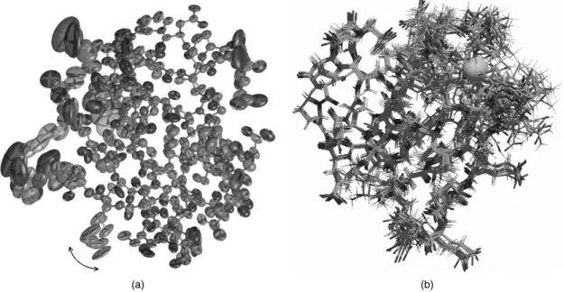
To make the point about 3D structures being merely models it is instructive to con-sider the subtly different types of model obtained by the two principal experimental techniques: X-ray crystallography and NMR spectroscopy. Figure 14.1 shows the two different interpretations of the same protein that are given by the two methods, as explained below. The models are of the protein rubredoxin with a bound zinc ion held in place by four cysteines.

Models from X-Ray Crystallography

Figure 14.1a is a representation of the protein model as obtained by X-ray crystallog-raphy. It is not a standard depiction of a protein structure; rather, its aim is to illustrate some of the components that go into the model. The components are: the x-, y-, z -coordinates, theB-factors, and occupancies of all the individual atoms in the structure. These parameters, together with the theory that explains how X-rays are scattered by the electron clouds of atoms, aim to account for the observed diffraction pattern. The x-,y-,z-coordinates define the mean position of each atom, whereas itsB-factor and occupancy aim to model its apparent disorder about that mean. This disorder may be the result of variations in the atom’s position in time, due to the dynamic motions of the molecule, or variations in space, corresponding to differences in conformation from one location in the crystal to another, or both. The higher the atom’s disorder, the more “smeared out” its electron density. B-factors model this apparent smearing around the atom’s mean location; at high resolution a better fit to the observations can often be obtained by assuming theB-factors to be anisotropic, as represented by the ellipsoids in Figure 14.1a. Occasionally, the data can be explained better by assuming that certain atoms can be in more than one place, due, say, to alternative conformations of a particular side chain (indicated by the arrows showing the two alternative positions of the glutamate sidechain in Figure 14.1a). The atom’s occupancy defines how often it is found in one conformation and how often in another (for example, in the example

(a) (b)

Figure 14.1. The different types of model generated by X-ray crystallography and NMR spec-troscopy. Both are representations of the same protein: rubredoxin. (a) In X-ray crystallography the model of a protein structure is given in terms of atomic coordinates, occupancies, and

B-factors. The side chain of Glu50 has two alternative conformations, with the change from one conformation to the other identified by the double-headed arrow. TheB-factors on all the atoms are illustrated by ‘‘thermal ellipsoids,’’ which give an idea of each atom’s anisotropic displacement about its mean position. The larger the ellipsoid, the more disordered the atom. Note that the main-chain atoms tend to be better defined than the side-chain atoms, some of which exhibit particularly large uncertainty of position. The region around the bound zinc ion appears well ordered. This is in stark contrast with the NMR case below. The coordinates andB-factors come from PDB entry 1irn, which was solved at 1.2 ˚A and refined with anisotropicB-factors. (b) The result of an NMR structure determination is a whole ensemble of model structures, each of which is consistent with the experimental data. The ensemble shown here corresponds to 10 of the 20 structures deposited for as PDB code 1bfy. In this case the metal ion, is iron. The more disordered regions represent either regions that are more mobile, or regions with a paucity of experimental data, or a combination of both. The region around the iron-binding site appears particularly disordered. Both diagrams were generated with the help of the Raster3D program (Merritt and Bacon, 1997). Figure also appears in Color Figure section_•.

given in Figure 14.1a the occupancies of the two alternative conformations are 56% and 44%).

Models from NMR Spectroscopy

The data obtained from NMR experiments are very different, so the models obtained differ in their nature, too. The spectra measured by NMR provide a diversity of infor-mation on the average structure of the molecule, and its dynamics, in solution. The most numerous, but often least precise, data are from NOESY• experiments where the intensities of particular signals correspond to the separations between spatially close

protons (≤6 ˚A) in the structure. The spectra from COSY-type• experiments give more precise information on the separations of protons up to three covalent bonds apart, and in some cases on the presence, or even length, of specific hydrogen bonds. Recently developed dipolar-coupling experiments give information on the relative orientation of particular backbone covalent bonds (Clore and Gronenborn, 1998).

For the vast majority of NMR experiments, the sample of protein or nucleic acid is in solution, rather than in crystal form, which means that molecules that are difficult to crystallize, and hence impossible to solve by crystallography, can often be solved by NMR instead. The separations are converted into distance and angular restraints and models of the structure that are consistent with these restraints are generated using various techniques, most commonly molecular dynamics-based simulated annealing procedures similar to those used in X-ray structure refinement. The end result is not a single model, but rather an ensemble of models that are all consistent with the given restraints, as illustrated in Figure 14.1b.

The reasons for generating an ensemble of structures from NMR data are twofold. Firstly, the NMR data are relatively less precise and less numerous than experimen-tal restraints from X rays so that a diversity of structures are consistent with them. Secondly, the biomolecules may genuinely possess heterogeneity in solution.

For general use, an ensemble of models is rather more difficult to handle than a single model. Ensembles deposited in the Protein Data Bank (PDB) can typically com-prise 20 models. One of these is often designated as representative of the ensemble, or a separate file containing an average model may be deposited in addition to the ensem-ble. The separate average structure is energy minimized to counteract the unphysical bond lengths and angles that the averaging process introduces. Such a structure tends to have a separate PDB identifier from that of the ensemble—so the same structure, or rather the outcome of the same experiment, appears as two separate entries in the PDB. This is clearly potentially confusing and the use of separate files is now discouraged. The representative member of an ensemble is usually taken to be the structure that differs least from all other structures in the ensemble. An algorithmic Web-based tool called OLDERADO (http://neon.chem.le.ac.uk/olderado) allows you to select such a representative from an ensemble (•Kelley, Gardner, Sutcliffe, 1996), but no single algorithm is universally agreed upon.

AIM

The aim of this chapter is to demonstrate that not all structures are of equally high quality, usually because of the quality of the experimental data from which they were determined, and that care needs to be taken before using any structure to draw biological or other conclusions. When selecting data sets for deriving general principles about, say, protein structures it is important to filter out those that might give misleading results simply because they are unlikely to be sufficiently accurate or precise to contribute meaningful or correct data to the analysis.

It does seem slightly churlish to reject structures from consideration given the amount of time, care, and hard work the experimentalists have put into solving them. However, if you put unsound data into your analysis, you will get unsound conclusions out. This chapter hopes to explain the limitations of using 3D structures uncritically for structural bioinformatics purposes, and to provide some rules of thumb for weeding out the defective ones: what are the symptoms, what should you look for, and which structures should you reject?

ERROR ESTIMATION AND PRECISION

All scientific measurements contain errors. No measurement can be made infinitely precisely; so, at some point, say after so many decimal places, the value quoted becomes unreliable. Scientists acknowledge this by estimating and quoting standard uncertainties on their results. For example, the latest value for Boltzmann’s constant is 1.3806503(24)×10−23 _{J K}−1_{, where the two digits in brackets represent the standard} uncertainty (ors.u.) in the last two digits quoted for the constant.

Compare this with the situation we have in relation to the 3D structures of bio-logical macromolecules. Figure 14.2 shows a typical extract from the atom details section of a PDB file. It relates to a single amino acid residue (a lysine) and shows the information deposited about each atom in the protein’s structure.

Looking at only the columns representing thex-,y-,z-coordinates you will notice that each value is quoted to three decimal places. This• suggests a precision of 1 in 105_{. Similarly, the B-factors (in the final column) are each quoted to two decimal} places. Is it possible that the atomic positions and B-factors were really so precisely defined? What are the error bounds on these values? What are their s.u.s? Are the values accurate to the first place of decimals? The second? The third?

In fact, with the exception of a very few PDB structures, no error bounds are given. As at November 2001 there were 5 such exceptions out of 16,646 structures: one was a carbohydrate (cycloamylose, PDB code 1c58), three were marginally differing copies of the same 13-residue enterotoxin (1etl, 1etm and 1etn), and the fifth was the crystal structure of the 54-residue rubredoxin (4rxn). All had been solved at atomic resolution (ranging from 0.89 ˚A to 1.2 ˚A) and refined by the full-matrix least-squares method that is mentioned below.

Thus, in the overwhelming majority of cases one cannot tell how precisely defined the values are. Why is this so? What kind of scientific measurement is this? And how are we to judge how much reliance to place on the data given?

Error Estimates in X-Ray Crystallography

Estimation of Standard Uncertainties. In X-ray crystallography it is, in the-ory, possible to calculate the standard uncertainties of the atomic coordinates and

Atomic coordinates Atom number Atom name Residue number Residue name Occup-ancy x y z B-factor ATOM 1 N LEU 1 -15.159 11.595 27.068 1.00 18.46 ATOM 2 CA LEU 1 -14.294 10.672 26.323 1.00 9.92 ATOM 3 C LEU 1 -14.694 9.210 26.499 1.00 12.20 ATOM 4 O LEU 1 -14.350 8.577 27.502 1.00 13.43 ATOM 5 CB LEU 1 -12.829 10.836 26.772 1.00 13.48 ATOM 6 CG LEU 1 -11.745 10.348 25.834 1.00 15.93 ATOM 7 CD1 LEU 1 -11.895 11.027 24.495 1.00 13.12 ATOM 8 CD2 LEU 1 -10.378 10.636 26.402 1.00 15.12

Figure 14.2. An extract from a PDB file of a protein structure showing how the atomic coordinates and other information on each atom are deposited. The atoms are of a single leucine residue in the protein. The contents of each column are labeled above the column. It can be seen that thex-,y-,z-coordinates of each atom are given to three decimal places.

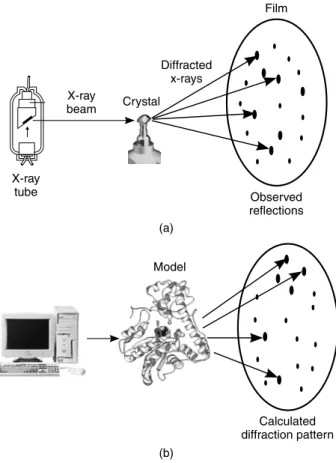
B-factors. In fact, it is routinely done for the crystal structures of small molecules such as those deposited in the Cambridge Structural Database (CSD; Allen et al., 1979). The calculations of the s.u.s are performed during the refinement stage of the structure determination. As you learned in Chapter 4, refinement involves modifying the initial model to improve the match between the experimentally determined structure factors—as obtained from the observed X-ray diffraction pattern—and the calculated structure factors—as obtained from applying scattering theory to the current model of the structure. Figure 14.3 illustrates this principle.

In practice refinement is usually a long drawn-out procedure requiring many cycles of computation interspersed here and there with manual adjustments of the model using molecular graphics programs to nudge the refinement process out of any local

(b) Model Calculated diffraction pattern (a) Film Observed reflections Diffracted x-rays X-ray beam X-ray tube Crystal

Figure 14.3. A schematic diagram illustrating the principle of structure refinement in X-ray crystallography. (a) X-rays are passed through a crystal of the molecule(s) of interest, generating a diffraction pattern from which, by one method or another (see Chapter 5), an initial model of the molecular structure is calculated. (b) Using the model, it is possible to apply scattering theory to calculate the diffraction pattern we would expect to observe. Usually this will differ from the experimental pattern. The process of structure refinement involves iteratively modifying the model of the structure until a better and better fit between the observed and calculated patterns is obtained. The goodness of fit of the two sets of data is measured by the reliability index, or

minimum that it may have become trapped in. Furthermore, because in protein crystal-lography the data-to-parameter ratio is poor (the data being the reflections observed in the diffraction pattern and the parameters being those defining the model of the protein structure: the atomic x-,y-,z-coordinates,B-factors, and occupancies) the data need to be supplemented by additional information. This extra information is applied by way of geometrical restraints. These are target values for geometrical properties such as bond lengths and bond angles and are typically obtained from crystallographic stud-ies of small molecules. The refinement process aims to prevent the bond lengths and angles in the model from drifting too far from these target values, which is achieved by applying additional terms to the function being minimized of the form:

Distances k=1

wk(dk0−dk)2,

where dk and dk0 are the actual and target distance, and wk is the weight applied to

each restraint.

If the structure is refined using full-matrix least-squares refinement, a by-product of this method is that thes.u.s of the refined parameters, such as the atomic coordinates andB-factors, can be obtained. However, their calculation involves inverting a matrix whose size depends on the number of parameters being refined. The larger the structure, the more atomic coordinates andB-factors, the larger the matrix. As matrix inversion is an ordern3 process, it has tended to be unfeasible for molecules the size of proteins and nucleic acids; these have several thousand parameters and consequently a matrix whose elements number several millions or tens of millions, which is why s.u.s have been routinely published for small-molecule crystal structures, but not for structures of biological macromolecules. It is purely a matter of size.

Recently, however, as faster workstations with larger memories have become avail-able, the situation has started to change, and calculation of atomic errors has become more practicable (Tickle, Laskowski, and Moss, 1998). Indeed,s.u.s are now frequently calculated for small proteins using SHELX (Sheldrick and Schneider, 1997), the refine-ment package originally developed for small molecules, but sadly, thes.u.data are still not commonly deposited in the PDB file. So this makes us none the wiser about the precision with which any given atom’s location has been determined.

So what is to be done? What information is there on the reliability of an X-ray crystal structure? What should one look for?

First of all, there are several parameters relating to the overall quality of the structure commonly cited in the literature that can be found in the header records of the PDB file itself, as described in Global Parameters for X-ray Structures.

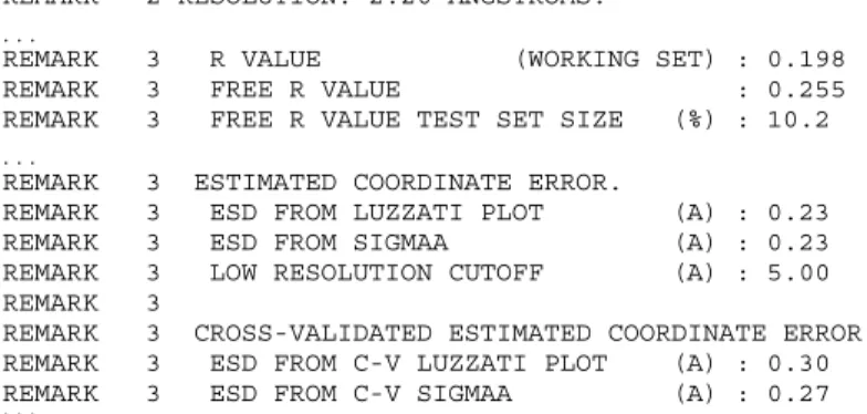
Global Parameters for X-ray Structures. Figure 14.4 shows an extract from the header records of a PDB file showing some of the commonly cited global parameters.

RESOLUTION. The resolution at which a structure is determined provides a mea-sure of the amount of detail that can be discerned in the computed electron density map. The reflections at larger scattering angles,θ, in the diffraction pattern correspond to higher resolution information coming as they do from crystal planes with a smaller interplanar spacing. The high-angle reflections tend to be of a lower intensity and more difficult to measure and, the greater the disorder in the crystal, the more of these high-angle reflections will be lost. Resolution is related to how many of these high-high-angle

REMARK 2 RESOLUTION. 2.20 ANGSTROMS.

REMARK 3 R VALUE (WORKING SET) : 0.198 REMARK 3 FREE R VALUE : 0.255 REMARK 3 FREE R VALUE TEST SET SIZE (%) : 10.2 REMARK 3 ESTIMATED COORDINATE ERROR.

REMARK 3 ESD FROM LUZZATI PLOT (A) : 0.23 REMARK 3 ESD FROM SIGMAA (A) : 0.23 REMARK 3 LOW RESOLUTION CUTOFF (A) : 5.00 REMARK 3

REMARK 3 CROSS-VALIDATED ESTIMATED COORDINATE ERROR. REMARK 3 ESD FROM C-V LUZZATI PLOT (A) : 0.30 REMARK 3 ESD FROM C-V SIGMAA (A) : 0.27 ⋅ ⋅ ⋅

⋅ ⋅ ⋅

⋅ ⋅ ⋅ ⋅ ⋅ ⋅

Figure 14.4. Extracts from the header records of a PDB file (1ydv) showing some of the statistics pertaining to the quality of the structure as a whole. These include the resolution,R-factor,R_free, and various estimates average positional errors ranging from 0.23–0.30 ˚A. TheR_free has been calculated on the basis of 10.2% of the reflections removed at the start of refinement and not used during it.

reflections can be observed, although the value actually quoted can vary from crystal-lographer to crystalcrystal-lographer as there is no clear definition of how resolution• should be calculated. The higher resolution shells will tend to be less complete and some crystallographers will quote the highest resolution shell giving a 100% complete data set, whereas others may simply cite the resolution corresponding to the highest angle of scatter observed.

The higher the resolution the greater the level of detail, and hence the greater the accuracy of the final model. The resolution attainable for a given crystal depends on how well ordered the crystal is—that is, how close the unit cells throughout the crystal are to being identical copies of one another. A simple rule of thumb is that the larger the molecule the lower will be the resolution of data collected.

Figure 14.5 shows an example of how the electron density for a single side chain improves as resolution increases. In general, side chains are difficult to make out at very low resolution (4 ˚A or lower), and the best that can be obtained is the overall shape of the molecule and the general locations of the regions of regular secondary structure. Models at such low resolution are clearly of no use for investigating side-chain conformations or interactions! At 3 ˚A resolution, the path of a protein’s chain can be traced through the density and at 2 ˚A the side chains can be confidently fitted.

The most precise structures are the atomic resolution ones (from around 1.2 ˚A resolution up to around 0.9 ˚A). Here the electron density is so clear that many of the hydrogen atoms become visible, and alternate occupancies become more easily dis-tinguishable. These structures require fewer geometrical constraints during refinement and hence give a better indication of the true geometry of protein structures.

The resolution of structures in the PDB varies from atomic resolution structures to very low resolution structures at around 4.0 ˚A, with a definite peak at around 2.0 ˚A. The lowest quoted resolution as of November 2001 was 30.0 ˚A for PDB entry 1qgc—the structure of the capsid protein of the foot-and-mouth virus, complexed with antibody, and solved by a combination of cryoelectron microscopy and X-ray crystallography (Hewat et al., 1997).

(a)

(b)

(c)

Figure 14.5. The effect of resolution on the quality of the electron density. The three plots show the electron density, as the green wire-frame cage, surrounding a single tyrosine residue. The residue is Tyr100 from concanavalin A as found in three PDB structures solved at (a) 3.0 ˚A resolution (PDB code 1val), (b) 2.0 ˚A (1con), and (c) 1.2 ˚A (1jbc). At the lowest resolution the electron density is merely a shapeless blob, but as the resolution improves the individual atoms come into clear focus. The electron density maps were taken from the Uppsala Electron Density Server (http://portray.bmc.uu.se/eds) and rendered using BobScript (Esnouf, 1997) and Raster3D (Merritt and Bacon, 1997)•.

Resolution is probably the clearest measure of the likely quality of the given model. However, bear in mind that, because there is no single definition of resolution, it tends not to be used consistently and its value can be overstated (Weissig and Bourne, 1999).

R-factor. TheR-factor is a measure of the difference between the structure factors calculated from the model and those obtained from the experimental data. In essence, it is a measure of the differences in the observed and computed diffraction patterns schematically illustrated in Figure 14.3. Higher values correspond to poorer agreement with the data, whereas lower values correspond to better agreement. Typically, for protein and nucleic acid structures, values quoted for theR-factor tend to be around 0.20 (or equivalently, 20%). Values in the range 0.40 to 0.60 can be obtained from a totally random structure, so structures with such values are unreliable and probably would never be published. Indeed, 0.20 seems to be something of a magical figure and many structures are deemed finished once the refinement process has taken the R-factor to this mystical value.

As a reliability measure, however, the R-factor is itself somewhat unreliable. It is quite easily susceptible to manipulation, either deliberate or unwary, during the refinement process, and so models with major errors can still have reasonable-looking R-factors. For example, one of the early incorrect structures, cited by Br¨and´en and Jones (1990), was that of ferredoxin I, an electron transport protein. The fully refined structure was deposited in 1981 as PDB code 2fd1, with a quoted resolution of 2.0 ˚A and anR-factor of 0.262. Due to the incorrect assignment of the crystal space group during the analysis of the X-ray diffraction data, this structure turned out to be completely wrong. The replacement structure, reanalyzed by the original authors and having the correct fold, was deposited as PDB entry 3df1 in 1988. Its resolution was given as 2.7 ˚A and itsR-factor as 0.35. On the face of it, therefore, mere comparison of the resolution and R-factor parameters would lead one to believe the first of the two structures to be the more reliable! The reason that anR-factor as low as 0.262 was achieved for a totally incorrect structure was that the coordinates included 344 water molecules, many extending far out from the protein molecule itself. This is a large number of waters for a protein containing only 107 residues. A rule of thumb suggested by Br¨and´en and Jones (1990) is that, for high-resolution structures, one water molecule for each residue is reasonable, and waters should only be added to the structure if they make plausible hydrogen bonds.

Incidentally, the version of ferredoxin that was 3df1 was itself twice superseded, first by entry 4df1 in mid-1988 and then by entry 5df1 in 1993. The last of these had a quoted resolution of 1.9 ˚A andR-factor of 0.215.

The ferredoxin example is one of overfitting; that is, having too many parameters for the experimental data available. It is always possible to fit a model, however wrong, to the data if there is an excess of parameters over observations.

Rfree. A more reliable measure is Br¨unger’s freeR-factor, orRfree(Br¨unger, 1992). This is less susceptible to manipulation during refinement. It is calculated in the same way as the standardR-factor and again measures the agreement between the structure factors as calculated from the model and as obtained from the experimental data. It differs in that its calculation uses only a small fraction of the experimental data, typically 5–10%, and, crucially, this fraction is excluded from the structure refinement procedure. The test set, as it is called, thus provides an independent measure of the goodness of fit of the model to the data while the refinement proceeds on the remaining

data, the working set. Unless there are correlations between the data in the test set and those in the working set, the refinement process should not be able to influence the Rfree measure.

The value ofRfree will tend to be larger than theR-factor, although it is not clear what a good value might be. Br¨unger has suggested that any value above 0.40 should be treated with caution (Br¨unger, 1997). There were approximately 20 structures in this category in the PDB, as of November 2001. Not surprisingly, most are fairly low-resolution structures (3.0–4.0 ˚A).

AVERAGEPOSITIONALERROR. Even though atomic coordinates.u.s are not com-monly given, it is quite usual for an estimate of the average positional error of a structure’s coordinates to be cited. There are two principal methods for estimating the average positional errors: the Luzzati plot (Luzzati, 1952) and theσAplot (Read, 1986).

The Luzzati plot is obtained by partitioning the reflections from the diffraction pattern into bins according to their value of sinθ, whereθis the reflection’s scattering angle, and then calculating theR-factor for each bin. The value calculated for each bin is plotted as a function of sinθ/λ, where λ is the wavelength of radiation used. The resulting plot is compared against the theoretical curves of Luzzati (1952) to obtain an estimate of the average positional error. One problem with this method is that the actual curves do not usually resemble the theoretical ones at all well, and so the error estimate is somewhat crude and often merely provides an upper limit on the error. Better results are obtained if the Rfree is used instead of the traditionalR-factor.

The σA plot provides a better estimate still. It involves plotting ln σA against

(sinθ/λ)2_{, where σ}

A is a complicated function that has to be estimated for each

(sinθ/λ)2 bin, as described in Read (1986). The resultant plot should give a straight line whose slope provides an estimate of the average positional error.

Most refinement programs compute both error estimates from the Luzzati and Read methods, so these values are commonly cited in the PDB file. You will find them in the file’s header records under the now unfashionable term “estimated standard deviation” (or ESD)—see Figure 14.4.

Bear in mind that an averages.u.is exactly what it says: an average over the whole structure. Thes.u.s of the atoms in the core of the molecule, which tends to be more ordered, will be lower than the average, while those of the atoms in the more mobile and less well-determined surface—and often more biologically interesting—regions will be higher than the average.

ATOMICB-FACTORS. A more direct, albeit merely qualitative, way of determining the precision of a given atom’s coordinates is to look at its associated B-factor. B -factors are closely related to the positional errors of the atoms, although the relationship is not a simple one that can be easily formulated (Tickle, Laskowski, and Moss, 1998). It is safe to say, however, that atoms in a structure with the largest B-values will also be those having the largest positional uncertainty. So if high levels of precision are required in your analysis, leave out the atoms having the highest B-factors. As a rule of thumb, atoms with B-values in excess of 40.0 are often excluded as being too unreliable. Similarly, if atoms in your region of interest, such as an active site, are all cursed with highB-factors then your region of interest is not well determined and you will need to be careful about the conclusions you draw from it.

Rules of Thumb for Selecting X-Ray Crystal Structures. Many analyses in structural bioinformatics require the selection of a dataset of 3D structures on which

to perform one’s analysis. A commonly used rule of thumb for selecting reliable struc-tures for such analyses, where reasonably accurate models are required, is to choose those models that have a quoted resolution of 2.0 ˚A or better, and an R-factor of 0.20 or lower. These criteria will give structures that are likely to be reasonably reli-able down to the conformations of the side chains and local atom–atom interactions. One example that uses such a dataset is the Atlas of Protein Side-Chain Interac-tions (http://www.biochem.ucl.ac.uk/bsm/sidechains), which depicts how amino acid sidechains pack against one another within the known protein structures.

Of course, it•really depends on the type of analysis required. For some analyses only atomic resolution structures (i.e., 1.2 ˚A or better) will do, as in the accurate deriva-tion geometrical properties of proteins—for example, side-chain torsional conformers and their standard deviations (EU 3-D Validation Network, 1998), or fine details of the peptide geometry in proteins that can reveal subtle information about their local electronic features (Esposito, et al., 2000). For other types of analysis, structures solved down to 3 ˚A may be good enough, as in any comparison of protein folds. One inter-esting example is that of the lactose operon repressor. Three structures of this protein were solved to 4.8 ˚A resolution, giving accurate position for only the protein’s Cα_atoms

(Lewis• et al., 1996). However, because the three structures were of the protein on its own, of the protein complexed with its inducer, and of the protein complexed with DNA, the global differences between the three structures showed how the protein’s conformation changed between its induced and repressed states. Thus even very low resolution structures were able to help explain how this particular protein achieves its biological function (Lewis•et al., 1996).

Often the above rule of thumb (resolution≤2.0 ˚A, andR-factor≤0.20) is supple-mented by a check on the year when the structure was determined. Structures are more likely to be less accurate the older they are simply because experimental techniques have improved markedly since the early pioneering days of the 1960s and 1970s. Indeed, many of the early structures have been replaced by more recent and accurate determinations.

Error Estimates in NMR Spectroscopy

The theory of NMR spectroscopy does not provide a means of obtainings.u.s for atomic coordinates directly from the experimental data, so estimates of a given structure’s accuracy and precision have to be obtained by more indirect means.

Global Parameters for NMR Structures. As mentioned above, a number of models can be derived that are compatible with the NMR experimental data. It is difficult to distinguish whether this multiplicity of models reflects real motion within the molecules or simply results from insufficient experimentally derived restraints. (Compare how the most poorly defined regions of the X-ray model of rubredoxin in Figure 14.1a do not necessarily correspond to the most poorly defined regions of the NMR model in Figure 14.1b, although remembering that one structure was in crystal form and the other in solution). Generally, the agreement of NMR models with the NMR data is measured by the agreement between the distance and angular restraints applied during refinement of the models and the corresponding distances and angles in the final models. Large numbers of severe violations would indicate a serious problem of data interpretation and model building.

However, the errors associated with the original experimental data are sufficiently large that it is almost always possible to generate models that do not violate the

restraints, or do so only slightly. Consequently, it is not possible to distinguish a merely adequate model from an excellent one by looking for restraint violations alone. Traditionally, the quality of a structure solved by NMR has also been measured by the root=mean=squaredeviation (rmsd) across the ensemble of solutions. Regions with high rmsd values are those that are less well defined by the data. In principle, such rmsd measures could provide a good indicator of uncertainty in the atomic coordinates; however, the values obtained are rather dependent on the procedure used to generate and select models for deposition. An experimentalist choosing the best few structures for deposition from a much larger draft ensemble can result in very misleading statis-tics for the PDB entry. For example, the best few structures may, in effect, be the same solution with minor variations—so the rmsd values will be small. Structures further down the original list may provide alternative solutions, which are slightly less con-sistent with the data, but that are radically different. The sizes of ensembles deposited in the PDB range from 1 to 85 models (as of November 2001).

The number of experimentally derived restraints per residue can give an indication of how effectively the NMR data define the structure in a manner analogous to the resolution of X-ray structures. Indeed, the number of restraints per residue correlates with the stereochemical quality of the structures to an extent, but some restraints may be completely redundant and no consistent method of counting is used by depositors. None of these measures gives a true indication of the accuracy of the models, that is, how well they represent the true structure, and few are reported in the PDB file.

In recent years, NMR equivalents of the crystallographicR-factor have been intro-duced. One method involves the use of dipolar couplings. These provide long-range structural restraints that are independent of other NMR observables such as the NOEs•, chemical shifts, and couplings constants that result from close spatial proximity of atoms. Because the expected dipolar couplings can be computed for a given model, this• provides a means of comparing observed with expected, and obtaining an R -factor that is a measure of the difference between the two (Clore and Garrett, 1999). What is more, it is also possible to obtain a cross-validatedR-factor, equivalent to the crystallographicRfree, wherein a subset of dipolar couplings are removed prior to the start of structure refinement and used only for computing the R-factor. This gives an unbiased measure of the quality of the fit to the experimental data. However, in the case of NMR, one cannot use a single test set of data; one has to perform a complete cross-validation. The reason for this is that, whereas in crystallography each reflec-tion contains informareflec-tion about the whole molecule, in NMR each dipolar coupling does not. So a complete cross-validation is required, which means that a number of calculations have to be performed, each using a different selection of test sets and working data sets; the test set, which usually comprises 10% of the whole data set, being selected at random each time.

Another technique for calculating an NMRR-factor uses the NOEs and involves back-calculation of the NMR intensities from the models obtained and comparison with those observed in the experiment. This technique is implemented in the program RFAC (Gronwald et al., 2000), which calculates not only an overall R-factor for the entire structure, but also local R-factors, including residue-by-residue R-factors and individual R-factors for different groups of NOEs (e.g., medium-range NOEs, long-range NOEs, interresidue NOEs, etc.).

An additional back-calculation method for checking structure quality is to calculate the expected frequencies (positions) of spectral peaks from the structure and compare them to those observed. This comparison• has the advantage that the frequencies are

not usually a target of the structure refinement procedure (Williamson, Kikuchi, and Asakura, 1995).

However, the measures described here are not yet generally included in the depo-sited PDB files.

Rules of Thumb for Selecting NMR Structures. Historically, the rule of thumb for selecting NMR structures for inclusion in structural analyses has been the simple one of excluding them altogether! This early prejudice stems from the fact that they were viewed as being of generally lower quality than X-ray structures, there was no easy way of selecting them with a consistent rule as that used for selecting X-ray structures, and they represented only a minority of the PDB anyway. However, nowadays NMR structures provide much valuable information about protein and DNA structures not available from X-ray studies. Indeed, although only about one in eight PDB structures come from NMR experiments (as at November 2001), in data sets of representative structures (Hobohm and Sander, 1994) around one in four are NMR structures. This result• stems from the fact that many unique and important proteins can only be solved by NMR.

Nevertheless, it is still not possible to differentiate between reliable and unreliable NMR structures from the information given in the PDB files. There is no standardized information provided that is akin to the resolution,R-factor, and estimated s.u.s rou-tinely quoted for X-ray crystal structures. The only way to get an idea of the quality of the structure is to read the paper describing it and judge from the statistics provided there or, more ambitiously, to carry out your own analysis of either the stereochemistry of the structure (using the programs that will be described later in this chapter) or the agreement between restraints and structures in those cases where the experimental data has been deposited along with the structure.

ERRORS IN DEPOSITED STRUCTURES Serious Errors

There have been a number of serious errors in X-ray and NMR structures documented in the literature (for references see Br¨and´en and Jones, 1990; Kleywegt, 2000). Many of the erroneous models have been retracted by their original authors, or replaced by improved versions. Structures are often re-refined, or solved with better data, and the models in the PDB are replaced by the improved versions.

The models that are replaced do not completely disappear, though. There is a grow-ing graveyard of obsolete structures—some very, very incorrect, others merely slightly mistaken—available at the Archive of Obsolete PDB Entries (http://pdbobs.sdsc.edu). This Web site provides a graphic history of each structure, some of which have gone through several incarnations (e.g., 1atc, which has been replaced in turn by 3atc, 5atc, 7atc, and 5at1).

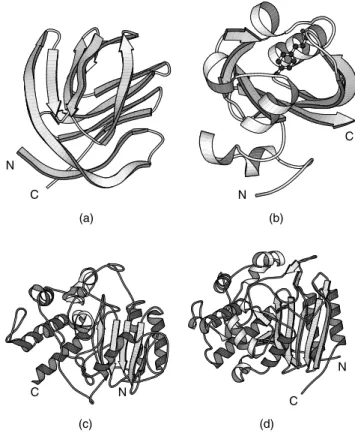
Of all errors, the most serious are those where the model is, essentially, completely wrong; for example, the trace of the protein chain follows the wrong path through the electron density and the resultant model has the wrong fold completely. Figures 14.6a and 14.6b give an example of such a case. There is practically no similarity between the correct and incorrect models.

The next most serious errors are where all, or most, of the secondary structural elements have been correctly traced, but the chain connectivity between them is wrong.

N C (c) N C (d) N C (a) N C (b)

Figure 14.6. Examples of seriously wrong protein models and their corrected counterparts. (a) Incorrect model of photoactive yellow protein (PDB code, 1phy, an all-Cα _{atom model), and}

(b) the corrected model (2phy, all atoms plus bound ligand). Superposition of the two models gives an rmsd of 15 ˚A between equivalent Cα_{atoms. Such a high value is hardly surprising given that}

the folds of the two models are so completely different. (c) Incorrect model of D-alanyl-D-alanine peptidase (1pte, an all-Cα _{atom model), and (d) corrected model (3pte, all atoms). The initial}

model had been solved at low resolution (2.8 ˚A) at a time when the protein’s sequence was unknown, so tracing the chain had been much more difficult than usual. Many of the secondary structure elements were correctly detected, but incorrectly connected. The matching secondary structures are shown in color: red for helices, and yellow for strands. The connectivity between them is completely different in the two models, with the earlier model having completely wrong parts of the sequence threaded through the secondary structure elements. Indeed, you can see that the central strand of theβ–sheet runs in the opposite direction in the two models. The N-and C-termini of all models are indicated. All plots were generated using the MOLSCRIPT program (Kraulis, 1991).

An example is given in Figures 14.6c and 14.6d. Here the erroneous model has most of the correct secondary structure elements, and has them arranged in the correct architecture. However, the protein sequence has been incorrectly traced through them (in one case going the wrong way down a β–strand). Thus most of the protein’s residues are in the wrong place in the 3D structure. Such errors arise because the loop regions that connect the secondary structure elements tend to be more flexible, and more disordered, so their electron density tends to be more poorly defined and

difficult to interpret correctly. This situation was particularly true in the case shown in Figure 14.6c as theprimary sequence of the protein was unknown at the time the structure was being solved and had to be guessed from the limited clues in the electron density map.

Less serious are frame-shift errors, although they can often result in a significant part of the model being incorrect. These errors occur where a residue is fitted into the electron density that belongs to the next residue. The frame shift persists until a compensating error is made when two residues are fitted into the density belonging to a single residue. These mistakes often occur at turns in the structure, and almost exclusively at very low resolution (3 ˚A or lower).

The least serious model-building errors involve the fitting of incorrect main-chain or side-chain conformations into the density. Of course, even such errors, depending on where they occur, can have an effect of the biological interpretation of what the structure does and how it does it.

Typical Errors

Typically, the models deposited in the PDB will be essentially correct. The remaining errors will be the random errors associated with any experimental measurement. As mentioned above for X-ray structures, the averages.u.s—estimated on the basis of the Luzzati andσAplots—can provide an idea of the magnitude of these errors. The values

range from around 0.01 ˚A to 1.27 ˚A. Note that the latter value approaches the length of some covalent bonds! The median of the quoted s.u.s corresponds to estimated average coordinate errors of around 0.28 ˚A. It has to be remembered that these values are estimates, and apply as an average over the whole model.

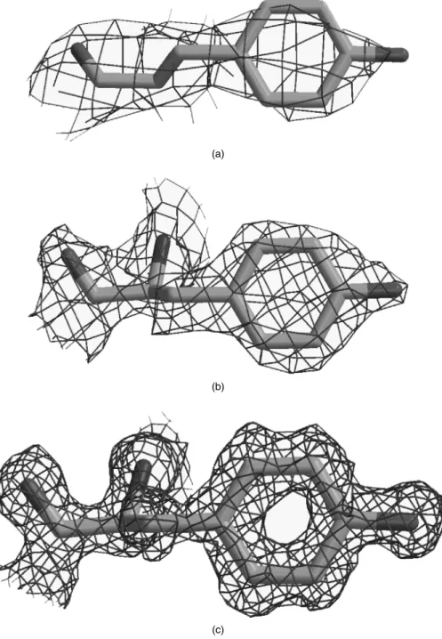
Figure 14.7 gives a feel of some typical uncertainties in atomic positions.

Stereochemical Parameters

An alternative way of assessing a structure’s quality, which complements the types of checks described so far, is to examine its geometry, stereochemistry, and other structural properties. A number of tests can be applied to a protein or nucleic acid structure that compare it against what is known about these molecules. This knowledge comes from systematic analyses of the existing structures in the PDB. In other words, the vast body of structures that have been solved to date provides a knowledge base of what is normal for proteins and nucleic acids.

The advantage of such tests of normality is that they do not require access to the original experimental data. Although it is possible to obtain the experimental data for many PDB entries—structure factors in the case of X-ray structures, and dis-tance restraints for NMR ones—these entries are still the minority, and deposition of these data is still at the discretion of the depositors. Furthermore, to make use of the

> Figure 14.7. Examples of typical uncertainties in atomic positions for (a) ans.u.of 0.2 ˚A, (b) 0.3 ˚A, and (c) 0.39 ˚A. The protein is the same rubredoxin from Figure 14.1a. Of course, as shown in Figure 14.1a, the distribution of uncertainties would not normally be so uniform, with higher variability in the surface side-chain atoms than, say, the buried main-chain atoms. Figure also appears in Color Figure section•.

(a)

(c)

Figure 14.7. (Continued)

data requires appropriate software packages and expert know-how. The stereochemical tests, however, require no experimental data. So any structure, whether experimentally determined, or the result of homology modeling, molecular dynamics, threading, or blind guesswork can be checked. The software is freely available and easy to use and interpret. What is more, many of the results of such checks made on existing structures are readily available on the Web, as will be mentioned below.

Most of the tests described here apply exclusively to protein structures. Similar tests have been developed for DNA and for small molecules (hetero atom groups) that may be bound to protein or DNA. These will be mentioned later. The stereochemi-cal tests include bond lengths, bond angles, torsion angles, hydrogen bond energies, and so on.

Before describing the checks, one crucial point needs to be stressed at the start. The majority of the checks compare a given structure’s properties against what is the norm. Yet this norm has been derived from existing structures and could be the result of biases introduced by different refinement practices. Furthermore, outliers, such as an excessively long bond length or an unusual torsion angle, should not be construed as errors. They may be genuine—for example, as a result of strain in the conformation, say, at the active site. The only way of verifying whether oddities are errors or merely oddities is by referring back to the original experimental data. Indeed, the experimenters who solved the structure may already have done this, found the apparent oddity to be correct and commented to that effect in the literature.

Having said that, if a single structure exhibits a large number of outliers and oddi-ties, then it probably does have problems and can safely be excluded from any analyses.

Proteins

The Ramachandran Plot. Perhaps the best-known, and certainly the most pow-erful, check for the stereochemical quality of a protein structure is the Ramachandran plot (Ramachandran, Ramakrishnan, and Sasisekharan, 1963). This plot is of the ψ main-chain torsion angle versus the φ main-chain torsion angle for every amino acid residue in the protein (except the two terminal residues, because the N-terminal residue has noφand the C-terminus has noψ). In the resulting scatter plot, the points tend to cluster in certain favorable regions, and tend to be excluded from certain disallowed regions due to steric hindrance of the side-chain atoms. Glycine and proline, which have no side chains as such, have slightly different distributions on the plot, although they too have regions from which they are excluded (Fig. 14.8).

Psi −180 ₋90 0 90 180 −90 0 90 0 90 180 Arg Phi −180 ₋90 0 90 180 −90 180 Gly Phi 0 90 Psi −180 −90 0 90 180 −90 180 Pro Phi

Figure 14.8. Differences in Ramachandran plots for (a) arginine, representing a fairly standard amino acid residue, (b) glycine that, due to its lack of a side chain, is able to reach the parts of the plot that other residue cannot reach, and (c) proline that, due to its restraints on the movement of the main chain, has a restricted range ofφvalues. The darker regions correspond to the more densely populated regions as observed in a representative sample of protein structures.

The favorable regions correspond to the regular secondary structures: right-handed helices, extended conformation (as found inβ-strands), and left-handed helices. Even residues in loops tend to lie within these favored regions. Figure 14.9a shows a typical Ramachandran plot,. The residues show a tight clustering in the most favored regions with few or none in the disallowed regions. The regions themselves have been deter-mined from an analysis of torsion angles in existing structures in the PDB (see, for example, Morris et al., 1992, or Kleywegt and Jones, 1996).

Figure 14.9b, shows a pathological Ramachandran plot. It comes from a structure that shall remain nameless. Here the majority of the residues lie in the disallowed regions, and it can be confidently concluded that the model has serious problems.

One caveat concerns proteins containing D-amino acids rather than the more com-mon L-amino acids. These residues have the opposite chirality so their φ–ψ values will be negative with respect to their L-amino cousins. The Ramachandran plot for D-amino acids is the same as for L-amino acids, but with every point reflected through the origin. Thus, proteins such as gramicidin A (e.g., PDB code 1grm) that have many D-amino acids, give Ramachandran plots that look particularly troubling but that may be perfectly correct.

Few models are as extreme as the one in Figure 14.9b. The tightness of clustering tends to be a function of resolution, with atomic resolution structures exhibiting very tight clustering (EU 3-D Validation Network, 1998). At lower resolution, as the data quality declines and the model of the protein structure becomes less accurate, so the points on the Ramachandran plot tend to disperse and more of them are likely to be found in the disallowed regions.

One feature that makes the Ramachandran plot such a powerful indicator of protein structure quality is that it is difficult to fool (unless one does so intentionally by, say, restraining φ–ψ values during structure refinement as is sometimes done for NMR structures). This reliability• was demonstrated by Gerard Kleywegt in Uppsala who once attempted to deliberately trace a protein chain backwards through its electron density to see whether it would refine and give the sorts of quality indicators that could fool people into believing it to be a reasonable model (Kleywegt and Jones, 1995). Of the parameters that he tried to fool, the two that seemed least gullible were theRfree factor mentioned above and the Ramachandran plot. The latter looked most

> Figure 14.9. Ramachandran plots for (a) a typical protein structure, and (b) a poorly defined protein structure. Each residue’sφ–ψ combination is represented as a black or red box, except for glycine residues, which are shown as black triangles. The red regions correspond to the most favorable, or core, regions (labeled A forα–helix, B forβ–sheet and L for left-handed helix) where the majority of residues should be found. The progressively lighter regions are the less-favored zones, with the white region corresponding to disallowedφ–ψcombinations for all but glycine residues. Residues falling within these disallowed regions are shown by the labeled red squares. The plot inais for PDB code 1ubi, which is of the chromosomal protein ubiquitin. All but one of the protein’s 66 nonglycine and nonproline residues are in the core regions of the Ramachandran plot (giving a core percentage of 98.5%). What is more, the points cluster reasonably well in the core regions. The structure was solved by X-ray crystallography at a resolution of 1.8 ˚A. The plot in

bexhibits many deviations from the core regions. The structure was solved by NMR, in the early days of the technique, and has a core percentage of 6.8%, while over a third of its residues lie in the disallowed regions. The plots were obtained using the PROCHECK program•.

unhealthy, with several residues in disallowed regions and no significant clustering in the most highly favored regions.

A simple measure of quality that can be derived from the plot is the percentage of residues in the most favorable or core regions. (Glycines and prolines are excluded from this percentage because of their unique distributions of availableφ–ψ combinations).

B A L b a l p ~p ~b ~a ~l b ~b b ~b ~b −180 −135 −90 −45 0 45 90 135 180 Phi (degrees) (a) 0 −135 −90 −45 45 90 135 180 Psi (degrees) B A L b a l p ~p ~b ~a ~l b ~b b ~b ~b VAL TYR VAL VAL ASP LYS MET ASP THR ILE THR VAL LEU VAL GLU THR TYR LYS HIS LEU ARG VAL LYS TYR SER

LYS _LYS ALA HIS

HIS ALA LYS ASP VAL LYS ILE MET SER LEU VAL GLU ILE VAL ALA VAL −135 −90 −45 0 45 90 135 180 −180 −135 −90 −45 0 45 90 135 180 Phi (degrees) (b) Psi (degrees)

Using the core regions defined by the PROCHECK program (see below), one generally finds that atomic resolution structures have well over 90% of their residues in these most favorable regions. For lower and lower resolution structures this percentage drops, with structures solved to 3.0–4.0 ˚A tending to have a core percentage around 70%. NMR structures also show increasing core percentage with increasing experimental information. However, NMR structures can have relatively good side-chain positions even with a poor core percentage as NMR data restrain side chains more strongly than the backbone because of the large number of side-chain protons.

Side-Chain Torsion Angles. Protein side chains tend to have preferred con-formations, known as rotamers, about their rotatable bonds, again as a result of steric hindrance. The rotamers are defined in terms of the side-chain torsion anglesχ1,χ2,χ3, and so. The first of these,χ1, is defined as the torsion angle about N—Cα—Cβ—Aγ, where Aγ _{is the next atom along the side chain (for example, in lysine the A}γ _atom

is Cγ_{). The next, χ}

2, is defined as Cα—Cβ—Aγ—Aδ, and so on. The χ1 and χ2 distributions are both trimodal with the preferred torsion angle values being termed gauche-minus (+60◦), trans (+180◦), and gauche-plus (−60◦). A plot of χ2 against χ1 for each residue has 3×3 preferred combinations, although the strength of each depends very much on the residue type. Figure 14.10 shows some examples of the distributions for different amino acid types.

Like the Ramachandran plot, a plot of the χ1–χ2 torsion angles can indicate problems with a protein model as these, like theφandψtorsion angles, tend not to be restrained during refinement. What is more, these torsion angles tend to cluster more tightly toward their ideal rotameric values as resolution improves (EU 3-D Validation Network, 1998). For example, the standard deviation of the χ1 torsion angles about their ideal position tends to be around 8◦ for atomic resolution structures and can go as high as 25◦ for structures solved at 3.0 ˚A. Similarly, the corresponding standard deviations for theχ2 torsion angles tend to be 10◦ and 30◦, respectively.

Bad Contacts. Another good check for structures to be wary of is the count of bad and unfavorable atom–atom contacts that they possess. Too many and the model may be a poor one.

The simplest checks are those which merely count bad contacts, that is, those where the distance between any pair of nonbonded atoms is smaller than the sum of their van der Waals radii. Furthermore, the atoms checked should not merely be those resulting in intraprotein contacts within the given protein structure; for X-ray crystal structures it is also necessary to consider atoms from molecules related by crystallographic and noncrystallographic symmetry.

More sophisticated checks consider each atom’s environment and determine how happy that atom is likely to be in that environment. For example, the ERRAT program

> Figure 14.10. Examples ofχ1–χ2distributions for six different amino acid residue types: Arg, Asn, Asp, His, Ile, and Leu. The darker regions correspond to the more densely populated regions as observed in a representative sample of protein structures. The dotted lines represent idealized rotameric torsion angles at 60◦, 180◦, and 300◦(equivalent to₋60◦). It can be seen that the true rotameric conformations differ slightly from these values and that the different side-chain types have very differentχ1–χ2distribution preferences.

0 90 180 270 360 90 180 270 360 Chi-1 Arg Chi-2 0 90 180 270 360 90 180 270 360 90 180 270 360 Chi-1 0 90 180 270 360 Chi-1 Asp His Chi-2 180 270 0 90 180 270 360 90 360 Chi-1 Asn 0 90 180 270 360 90 180 270 360 90 180 270 360 Chi-1 Leu 0 90 180 270 360 Chi-1 Chi-2 Ile

(Colovos and Yeates, 1993) counts the numbers of nonbonded contacts, within a cutoff distance of 3.5 ˚A, between different pairs of atom types. The atoms are classified as car-bon (C), nitrogen (N), and oxygen/sulfur (O), so there are six distinct interaction types: CC, CN, CO, NN, NO, OO. If the frequencies of these interaction types differ signif-icantly from the norms (as obtained from well-refined high-resolution structures) the protein model may be somewhat suspect. A similar analysis can be used to locate local problem regions by using a nine-residue sliding window and obtaining the interaction frequencies at each window position.

One level up in sophistication is the DACA method (Vriend and Sander, 1993), which is implemented in the WHAT IF program (Vriend, 1990). DACA stands for Directional Atomic Contact Analysis and compares the 3D environment surrounding each residue fragment in the protein with normal environments computed from a high-quality data set of protein structures. There are 80 different fragment types, including main-chain fragments as well as side-chain fragments. The environment of each frag-ment is essentially the count of different nonbonded atoms in each 1 ˚A×1 ˚A×1 ˚A cell of a 16 ˚A×16 ˚A×16 ˚A cube surrounding the fragment.

A similar approach is that of the ANOLEA program (Atomic NOn-Local Environ-ment AssessEnviron-ment), which calculates a nonlocal energy for atom–atom contacts based on an atomic mean force potential (Melo and Feytmans, 1998).

Other Parameters. Other parameters that can be used to validate protein struc-tures include counts of unsatisfied hydrogen bond donors and hydrogen-bonding ener-gies as is done in the WHATCHECK program mentioned below (Hooft et el., 1996). See also Chapter 15.

C-alpha Only Structures. As of November 2001, there were around 200 struc-tures in the PDB (out of over 16,000) that contain one or more protein chains for which only the Cα _{coordinates have been deposited. The deposition of C}α_{-only coordinate}

sets is usually done where the data quality has been too poor to resolve more of the structure. It was common in the early days of protein crystallography for only Cα_s

to be deposited; nowadays it is still quite common for only Cαs to be deposited for very large structures, such as the recently determined structure of the ribosome at 5.5 ˚A (PDB codes 1gix and 1giy).

The standard validation checks are of no use for such models, lacking as they are in so much of their substance. However, there is an equivalent to the Ramachandran plot for these structures (Kleywegt, 1997). The parameters plotted are the Cα_—Cα_—Cα_—Cα _{torsion angle as a function of the C}α_—Cα_—Cα _{angle for}

every residue in the protein. As with the Ramachandran plot, there are regions of this plot that tend to be highly populated, and others that appear forbidden. So a structure with many outliers in the forbidden zones should be treated with caution. The checks are incorporated in the program MOLEMAN2 which can be run over the Web (see Table 14.1).

Nucleic Acids

Finding validation tools for DNA and RNA is trickier than for proteins. The PDB’s validation tool, ADIT (AutoDep Input Tool), incorporates a program called NuCheck (Feng, Westbrook, and Berman, 1998) for validating the geometry of DNA and RNA. Binary versions of the ADIT package can be downloaded for use on SGI and Linux machines (see Table 14.2).

T A B L E 14.1. WWW Servers for Checking Structure Coordinates Online

Program Reference Protein/DNA URL

ANOLEA Melo and Feytmans,

1998 Protein www.fundp.ac.be/sciences/ biologie/bms/CGI/test.htm Biotech Validation: PROCHECK, PROVE, WHAT IF EU 3-D Validation Network, 1998 Protein biotech.embl-ebi.ac.uk:8400 biotech.embl-ebi.ac.uk:8400

DACA Vriend and Sander,

1993

Protein cmbi1.cmbi.kun.nl:1100/

WIWWWI/oldqua.html

ERRAT Colovos and Yeates,

1993

Protein www.doe-mbi.ucla.edu/

Services/ERRAT

MC-Annotate Gendron, Lemieux,

and Major, 2001

RNA www-lbit.iro.umontreal.ca/

mcannotate

MOLEMAN2 Kleywegt, 1997 Protein

(C-alpha only)

xray.bmc.uu.se/cgi-bin/gerard/ rama server.pl

Verify3D Bowie, L¨uthy and

Eisenberg, 1991

Protein www.doe-mbi.ucla.edu/

Services/Verify 3D

T A B L E 14.2. Programs for Checking Structure Coordinates

Program name Reference URL

ADIT PDB pdb.rutgers.edu/software

ERRAT Colovos and Yeates, 1993 www.doe-mbi.ucla.edu/People/Yeates/

Gallery/Errat.html

PROCHECK Laskowski et al., 1993 www.biochem.ucl.ac.uk/∼roman/

procheck/procheck.html

PROVE Pontius, Richelle, and Wodak,

1996

www.ucmb.ulb.ac.be/SCMBB/PROVE

SQUID Oldfield, 1992 www.yorvic.york.ac.uk/∼oldfield/

squidmain.html

WHATCHECK Hooft et al., 1996 www.cmbi.kun.nl/gv/whatcheck

WHAT IF Vriend, 1990 www.cmbi.kun.nl/whatif

A program specifically developed for checking the geometry of RNA structures, but that can also be used for DNA structures, is MC-Annotate (Gendron, Lemieux, and Berman, 2001). It computes a number of peculiarity factors, based on various metrics including torsion angles and root-mean-square deviations from standard conformations, that can highlight irregular regions in the structure that may be in error or merely under strain.

Hetero Groups

The geometry of hetero compounds, as deposited in structures in the PDB, tends to be of widely varying quality. The HETZE program (Kleywegt and Jones, 1998) is one of the few validation methods that checks various geometrical parameters of the hetero compounds associated with PDB structures. These parameters include bond lengths,

torsion angles, and some virtual torsion angles, the information principally coming from the small-molecule structures in the CSD (Allen et al., 1979).

Software for Quality Checks

A large number of programs are freely available that can perform the sorts of quality checks described above on proteins, nucleic acids, and hetero compounds. Below are listed the most commonly used programs not requiring any specialist knowledge or additional specialist software. Details of how to obtain the programs are given in Table 14.2.

PROCHECK. PROCHECK (Laskowski et al., 1993) computes a number of stereo-chemical parameters for a given protein model and outputs the results in easy-to-understand colored plots in PostScript format. Significant deviation in the parameters from the standards that have been derived from a database of well-refined high-resolution proteins are highlighted as being unusual. The plots include: Ramachandran plots, both for the protein as a whole and for each type of amino acid;χ1–χ2 plots for each amino acid type; main-chain bond lengths and bond angles; secondary structure plot; deviations from planarity of planar side chains; and so on.

WHATCHECK and WHAT IF. The WHATCHECK program (Hooft et al., 1996) is a subset of Gert Vriend’s WHAT IF package (Vriend, 1990). It contains an enormous number of checks and produces a long and very detailed output of discrepancies of the given protein structure from the norms. The DACA method, mentioned above, for analyzing nonbonded contacts, is incorporated into the original WHAT IF program.

PROVE. PROVE compares atomic volumes against a set of precalculated standard values (Pontius, Richelle, and Wodak, 1996). Volumes are calculated using Voronoi polyhedra to define the space that each atom occupies by placing dividing planes between it and its neighbors.

SQUID. The SQUID program (Oldfield, 1992) displays two-dimensional and three-dimensional data derived from protein structures using many graph types. It can also be used for validation via ready-to-use scripts.

ERRAT. The ERRAT program has already been described. It analyzes nonbonded atom contacts in protein structures in terms of CC, CN, CO, and so forth contacts.

QUALITY INFORMATION ON THE WEB

Rather than having to install and run one of the above packages, it is possible to obtain much of the information it provides from the Web. Several sites provide precomputed quality criteria for all existing structures in the PDB. Other sites allow you upload your own PDB file, via your Web browser, and will run their validation programs on it and provide you with the results of their checks.

PDBsum—PROCHECK Summaries

The first site that provides precomputed quality criteria is the PDBsum Web site (Laskowski, 2001) at http://www.biochem.ucl.ac.uk/bsm/pdbsum. This Web site spe-cializes in structural analyses and pictorial representations of all PDB structures. Each

structure containing one or more protein chains has a PROCHECK and a WHAT CHECK button. The former gives a Ramachandran plot for all protein chains in the structure, together with summary statistics calculated by the PROCHECK program. These results can provide a quick guide to the likely quality of the structure, in addition to the structure’s resolution,R-factor and, where available,Rfree.

The WHATCHECK button links to the PDBREPORT for the structure, described below.

Occasionally the model of a protein structure is so bad that one can tell immediately from merely looking at the secondary structure plot on the PDBsum page. Most proteins have around 50–60% of their residues in regions of regular secondary structure, that is, in α-helices and β–strands. However, if a model is really poor, the main-chain oxygen and nitrogen atoms responsible for the hydrogen-bonding that maintains the regular secondary structures can lie beyond normal hydrogen-bonding distances; so the algorithms that assign secondary structure (Chapter 17) may fail to detect some of the α-helices andβ–strands that the correct protein structure contains. Figure 14.11 gives an example of the secondary structure contents for a typical protein and for the protein that had the poor Ramachandran plot in Figure 14.9b.

A A b b b A H1 H2 A bb A b H3 MQIFVKTLTGKTITLEVEPSDTIENVKAKIQDKEGIPPDQQRLIFAGKQLEDGRTLSDYN 5 10 15 20 25 30 35 40 45 50 55 60 IQKESTLHLVLRLRGG 65 70 75 (a) A _{b b b} A b b b g gb b b 5 10 15 20 25 30 35 40 45 50 55 60 65 70 75 80 85 (b)

Figure 14.11. Schematic diagrams of two protein models in the PDB. (a) A typical protein showing an expected 50–60% of its residues inα–helices (shown schematically by the sawtooth regions) and β–strands (shown by arrows). (b) A poorly defined model that has hardly any regions of secondary structure at all. The labels and symbols correspond to various secondary structure motifs. Theβandγsymbols identifyβ- andγ–turns, while the red hairpinlike symbols correspond toβ–hairpins. The helices are labeled H1–H3 ina, and strands are labeled A for β-sheet A. The Ramachandran plots for both models are shown in Figure 14.7. The sequence of the protein inbhas been removed to hinder identification. The above plots were obtained from the PDBsum database•.