The {RDF}-3X Engine for Scalable Management of {RDF} Data

(1)

The RDF-3X Engine for

Scalable Management

of RDF Data

Thomas Neumann Gerhard Weikum MPI–I–2009–5-003 March 2009

(2)

Authors’ Addresses Thomas Neumann Max-Planck-Institut für Informatik Campus E1 4 66123 Saarbrücken Germany Gerhard Weikum Max-Planck-Institut für Informatik Campus E1 4 66123 Saarbrücken Germany

(3)

Abstract

RDF is a data model for schema-free structured information that is gaining momentum in the context of Semantic-Web data, life sciences, and also Web 2.0 platforms. The “pay-as-you-go” nature of RDF and the flexible pattern-matching capabilities of its query language SPARQL entail efficiency and scalability challenges for complex queries including long join paths. This paper presents the RDF-3X engine, an implementation of SPARQL that achieves excellent performance by pursuing a RISC-style architecture with streamlined indexing and query processing.

The physical design is identical for all RDF-3X databases regardless of their workloads, and completely eliminates the need for index tuning by exhaustive indexes for all permutations of subject-property-object triples and their binary and unary projections. These indexes are highly compressed, and the query processor can aggressively leverage fast merge joins with excellent performance of processor caches. The query optimizer is able to choose optimal join orders even for complex queries, with a cost model that includes statistical synopses for entire join paths. Although RDF-3X is optimized for queries, it also provides good support for efficient online updates by means of a staging architecture: direct updates to the main database indexes are deferred, and instead applied to compact differential indexes which are later merged into the main indexes in a batched manner.

Experimental studies with several large-scale datasets with more than 50 million RDF triples and benchmark queries that include pattern matching, manyway star-joins, and long path-joins demonstrate that RDF-3X can outperform the previously best alternatives by one or two orders of magnitude.

Keywords

RDF, batched updates, indexing, query processing, query optimization, SPARQL, database engine

(4)

1 Introduction

1.1 Motivation and Problem

The RDF (Resource Description Framework) data model has been around for a decade. It has been designed as a flexible representation of schema-relaxable or even schema-free information for the Semantic Web [41]. In the commercial IT world, RDF has not received much attention until recently, but now it seems that RDF is building up a strong momentum. Semantic-Web-style ontologies and knowledge bases with millions of facts from Wikipedia and other sources have been created and are available online [4, 56, 64]. E-science data repositories support RDF as an import/export format and also for selective (thus, query-driven) data extractions, most notably, in the area of life sciences (e.g., [7, 59]). Finally, Web 2.0 platforms for online communities are considering RDF as a non-proprietary exchange format and as an instrument for the construction of information mashups [24, 25, 43].

In RDF, all data items are represented in the form of (subject, predicate, object) triples, also known as (subject, property, value) triples. For example, information about the song “Changing of the Guards” performed by Patti Smith could include the following triples:

(id1, hasT ype, ”song”),

(id1, hasT itle, ”Changing of the Guards”), (id1, perf ormedBy, id2),

(id2, hasN ame,”P atti Smith”), (id2, bornOn,”December 30, 1946”), (id2, bornIn, id3),

(id3, hasN ame,”Chicago”), (id3, locatedIn, id4),

(id4, hasN ame,”Illinois”), (id1, composedBy, id5),

(id5, hasN ame,”Bob Dylan”), and so on.

(7)

resemble attributes, there is no database schema; the same database may contain triples about songs with predicates “performer”, “hasPerformed”, “sungBy”, “composer”, “creator”, etc. A schema may emerge in the long run (and can then

be described by the RDF Vocabulary Description Language). In this sense, the notion of RDF triples fits well with the modern notion of data spaces and its “pay as you go” philosophy [20]. Compared to an entity-relationship model, both an entity’s attributes and its relationships to other entities are represented by predicates. All RDF triples together can be viewed as a large (instance-level) graph.

The SPARQL query language is the official standard for searching over RDF repositories. It supports conjunctions (and also disjunctions) of triple patterns, the counterpart to select-project-join queries in a relational engine. For example, we can retrieve all performers of songs composed by Bob Dylan by the following SPARQL query:

Select ?n Where {

?p <hasName> ?n. ?s <performedBy> ?p.

?s <composedBy> ?c. ?c <hasName> "Bob Dylan"

}

Here each of the conjunctions, denoted by a dot, corresponds to a join. The whole query can also be seen as graph pattern that needs to be matched in the RDF data graph. In SPARQL, predicates can also be variables or wildcards, thus allowing schema-agnostic queries. For example,

RDF engines for storing, indexing, and querying have been around for quite a few years; especially, the Jena framework by HP Labs has gained significant pop-ularity [63], and Oracle also provides RDF support for semantic data integration in life sciences and enterprises [12, 40]. However, with the exception of the VLDB 2007 paper by Abadi et al. [1] (and very recent work presented at VLDB 2008 [37, 50, 61]), none of the prior implementations could demonstrate convincing efficiency, failing to scale up towards large datasets and high load. [1] achieves good performance by grouping triples with the same property name into property tables, mapping these onto a column store, and creating materialized views for frequent joins.

Managing large-scale RDF data includes technical challenges for the storage layout, indexing, and query processing:

1. The absence of a global schema and the diversity of predicate names pose major problems for the physical database design. In principle, one could rely on an auto-tuning “wizard” to materialize frequent join paths; however, in practice, the evolving structure of the data and the variance and dynamics of the workload turn this problem into a complex sisyphus task.

2. By the fine-grained modeling of RDF data – triples instead of entire records or entities – queries with a large number of joins will inherently form a large

(8)

part of the workload, but the join attributes are much less predictable than in a relational setting. This calls for specific choices of query processing algorithms, and for careful optimization of complex join queries; but RDF is meant for on-the-fly applications over data spaces, so the optimization takes place at query run-time.

3. As join-order and other execution-plan optimizations require data statistics for selectivity estimation, an RDF engine faces the problem that a suitable granularity of statistics gathering is all but obvious in the absence of a schema. For example, single-dimensional histograms on all attributes that occur in the workload’s where clauses – the state-of-the-art approach in relational systems – is unsuitable for RDF, as it misses the effects of long join chains or large join stars over many-to-many relationships.

4. Although RDF uses XML syntax and SPARQL involves search patterns that resemble XML path expressions, the fact that RDF triples form a graph rather than a collection of trees is a major difference to the more intensively researched settings for XML.

1.2 Contribution and Outline

This paper gives a comprehensive, scalable solution to the above problems. It presents a complete system, coined RDF-3X (for RDF Triple eXpress), designed and implemented from scratch specifically for the management and querying of RDF data. RDF-3X follows the rationale advocated in [28, 55] that data-management systems that are designed for and customized to specific application domains can outperform generic mainstream systems by two orders of magnitude. The factors in this argument include 1) tailored choices of data structures and algorithms rather than supporting a wide variety of methods, 2) much lighter software footprint and overhead, and as a result, 3) simplified optimization of system internals and easier configuration and self-adaptation to changing environments (e.g., data and workload characteristics).

RDF-3X follows such a RISC-style design philosophy [11], with “reduced instruction set” designed to support RDF. RDF-3X is based on three key principles:

• Physical design is workload-independent by creating appropriate indexes over a single “giant triples table”. RDF-3X does not rely on the success (or limitation) of an auto-tuning wizard, but has effectively eliminated the need for physical-design tuning. It does so by building indexes over all 6 permutations of the three dimensions that constitute an RDF triple, and additionally, indexes over count-aggregated variants for all three two-dimensional and all three one-two-dimensional projections. Each of these indexes can be compressed very well; the total storage space for all indexes together is less than the size of the primary data.

(9)

• The query processor is RISC-style by relying mostly on merge joins over sorted index lists. This is made possible by the “exhaustive” indexing of the triples table. In fact, all processing is index-only, and the triples table exists merely virtually. Operator trees are constructed so as to preserve

interesting orders [19] for subsequent joins to the largest possible extent; only when this is no longer possible, RDF-3X switches to hash-based join processing. This approach can be highly optimized at the code level, and has much lower overhead than traditional query processors. At the same time, it is sufficiently versatile to support also the various duplicate-elimination options of SPARQL, disjunctive patterns in queries, and all other features that SPARQL requires.

• The query optimizer mostly focuses on join orderin its generation of execu-tion plans. It employs dynamic programming for plan enumeraexecu-tion, with a cost model based on RDF-specific statistical synopses. These statistics include counters of frequent predicate-sequences in paths of the data graph; such paths are potential join patterns. Compared to the query optimizer in a universal database system, the RDF-3X optimizer is simpler but much more accurate in its selectivity estimations and decisions about execution plans.

Although it is reasonable to assume that most RDF databases are query-intensive if not read-only (e.g., large reference repositories in life sciences), there has to be support for at least incremental loading and ideally even online updates such as inserting a new triple for annotating existing data. The challenge in doing this efficiently is to deal with the aggressive indexing that RDF-3X employs for fast querying. We have developed a staging architecture that defers index updates. Updates are collected in workspaces and differential indexes, and are later merged into the main database indexes in a very efficient batched manner. This staging is transparent to programs; the query processor is appropriately extended to provide this convenience with low overhead. While this approach does not provide full-fledged ACID transactions, it includes simple but effective ways of concurrency control and recovery and supports the read-committed isolation level.

The scientific contributions of this work are:

1. a novel architecture for RDF indexing and querying, eliminating the need for physical database design;

2. an optimizer for large join queries over non-schematic RDF triples, driven by a new kind of selectivity estimation for RDF paths;

3. a new staging architecture for efficiently handling updates, with very good performance of batched updates;

(10)

4. a comprehensive performance evaluation, based on real measurements with three large datasets, demonstrating large gains over the previously best engine [1] (by a typical factor of 10 and up to 100 or more for some queries). The source code of RDF-3X and the experimental data are available for non-commercial purposes from the Web site [42].

A previous version of this work has been presented in [37]. The current paper extends this prior publication in two major ways: 1) we describe the algorithms for query compilation and query optimization, which are merely sketched in [37]; 2) we present a novel way of efficiently supporting updates to RDF-3X databases, and give performance measurements for multi-user workloads.

The rest of the paper is organized as follows. Section 2 provides background on RDF, SPARQL, and prior work on indexing and query processing. Section 3 presents our solution for the physical design of RDF repositories. Section 4 describes the architecture and algorithms of the RDF-3X query compiler and query processor. Section 5 covers the query optimization techniques used in RDF-3X. Section 6 discusses our solutions to selectivity estimation for SPARQL expressions. Section 7 shows how to efficiently support online updates and incremental loading in RDF-3X. Section 8 presents the results of our comprehensive performance evaluation and comparison to alternative approaches.

(11)

2 Background and State of the

Art

2.1 SPARQL

SPARQL queries [52] are pattern matching queries on triples that constitute an RDF data graph. Syntactic sugar aside, a basic SPARQL query has the form

select ?variable1 ?variable2 ... where { pattern1. pattern2. ... }

where eachpatternconsists ofsubject, predicate, object, and each of these is either a variable or a literal. The query model is query-by-example style: the query specifies the known literals and leaves the unknowns as variables. Variables can occur in multiple patterns and thus imply joins. The query processor needs to find all possible variable bindings that satisfy the given patterns and return the bindings from the projection clause to the application. Note that not all variables are necessarily bound (e.g., if a variable only occurs in the projection and not in a pattern), which results in NULL values.

This pattern matching approach restricts the freedom of the query engine with regard to possible execution plans, as shown in the following example:

select ?a ?c

where { ?a label1 ?b. ?b label2 ?c }

The user is interested in all ?a and ?c that are reachable with certain edges via ?b. The value of ?b itself is not part of the projection clause. Unfortunately the pattern matching semantics requires that nevertheless all bindings of ?b need to be computed. There might be multiple ways from ?ato ?c, resulting in duplicates in the output. As this is usually not what the user/application intends, SPARQL introduced two query modifiers: the distinct keyword specifies that duplicates must be eliminated, and thereduced keyword specifies that duplicates may but need not be eliminated. The goal of the reduced keyword was obviously to help

(12)

RDF query engines by allowing optimizations, but with thereduced option the query output has a nondeterministic nature.

Nevertheless, even the default mode of creating all duplicates allows some optimizations. The query processor must not ignore variables that are projected away due to their effect on duplicates, but it does not have to create the explicit bindings. As long as we can guarantee that the correct number of duplicates is produced, the bindings themselves are not relevant. We will use this observation later by counting the number of duplicates rather than producing the duplicates themselves.

2.2 Related Work

Most publicly accessible RDF systems have mapped RDF triples onto relational tables (e.g., RDFSuite [2, 44], Sesame [8, 39], Jena [26, 63], the C-Store-based RDF engine of [1], and also Oracle’s RDF MATCH implementation [12]). There are two extreme ways of doing this: 1) All triples are stored in a single, gianttriples tablewith generic attributes subject, predicate, object. 2) Triples are grouped by their predicate name, and all triples with the same predicate name are stored in the sameproperty table. The extreme form of property tables with a separate table for each predicate name can be made more flexible, leading to a hybrid approach: 3) Triples are clustered by predicate names, based on predicates for the same entity class or co-occurrence in the workload; eachcluster-property table contains the values for a small number of correlated predicates, and there may additionally be a “left-over” table for triples with infrequent predicates. A cluster-property table has a class-specific schema with attributes named after the corresponding RDF predicates, and its width can range from a single predicate (attribute) to all predicates of the same entity type.

Early open-source systems like Jena [26, 63] and Sesame [8, 39] use clustered-property tables, but left the physical design to an application tuning expert. Neither of these systems has reported any performance benchmarks with large-scale data in the Gigabytes range with more than 10 million triples. Oracle [40] has reported very good performance results in [12], but seems to heavily rely on good tuning by making the right choice of materialized join views (coined subject-property matrix) in addition to its basic triples table. The previously fastest RDF engine by [1] uses minimum-width property tables (i.e., binary relations), but maps them onto a column-store system. [57] gives a nice taxonomy of different storage layouts and presents systematic performance comparisons for medium-sized synthetic data and synthetic workload.

The scalable system of [1], published in the 2007 VLDB conference, kindled great interest in RDF performance issues and new architectures. In contrast to the arguments that [1] gives against the “giant-triples-table” approach, both RDF-3X [37] and HexaStore [61] recently showed how to successfully employ a

(13)

triples table with excellent performance. The work of [50] systematically studied the impact of column-stores (MonetDB) and row-stores (PostgreSQL) on different physical designs and identified strengths and weaknesses under different data and workload characteristics. The quest for scalable performance has also led to new benchmark proposals [45] and the so-called billion triples challenge [49].

The previously best performing systems, Oracle and the C-Store-based engine [1], rely on materialized join paths and indexes on these views. The indexes themselves are standard indexes as supported by the underlying RDBMS and column store, respectively. The native YARS2 system [22] proposes exhaustive indexes of triples and all their embedded sub-triples (pairs and single values) in 6 separate B+_{-tree or hash indexes. This resembles our approach, but YARS2} misses the need for indexing triples in collation orders other than the canonical order by subject, predicate, object (as primary, secondary, and tertiary sort criterion). A very similar approach is presented for the HPRD system [6] and available as an option (coined “triple-indexes”) in the Sesame system [39]. Both YARS2 and HPRD seem to be primarily geared for simple lookup operations with limited support for joins; they lack DBMS-style query optimization (e.g., do not consider any join-order optimizations, although [6] recognizes the issue). [5] proposes to index entire join paths using suffix arrays, but does not discuss optimizing queries over this physical design. [58] introduces a new kind of path indexing based on judiciously chosen “center nodes”; this index, coined GRIN, shows good performance on small- to medium-sized data and for hand-specified execution plans. Physical design for schema-agnostic “wide and sparse tables” is also discussed in [13], without specific consideration to RDF. All these methods for RDF indexing and materialized views incur some form of physical design problem, and none of them addresses the resulting query optimization issues over these physical-design features.

As for query optimization, [12, 40] and [1] utilize the state-of-the-art techniques that come with the SQL engines on which these solutions are layered. To our knowledge, none of them employs any RDF-native optimizations. [54] outlines a framework for algebraic rewriting, but it seems that the main rule for performance gains is pushing selections below joins; there is no consideration of join ordering. [23] has a similar flavor, and likewise disregards the key problem of finding good join orderings.

Recently, selectivity estimation for SPARQL patterns over graphs have been addressed by [54] and [31]. The method by [54] gathers separate frequency statistics for each subject, each predicate, and each object (label or value); the frequency of an entire triple pattern is estimated by assuming that subject, predicate, and object distributions are probabilistically independent. The method by [31, 32] is much more sophisticated by building statistics over a selected set of arbitrarily shaped graph patterns. It casts the selection of patterns into an optimization problem and uses greedy heuristics. The cardinality estimation of a query pattern identifies maximal subpatterns for which statistics exist, and combines them with

(14)

uniformity assumptions about super-patterns without statistics. While [54] seems to be too simple for producing accurate estimates, the method by [31] is based on a complex optimization problem and relies on simple heuristics to select a good set of patterns for the summary construction. The method that we employ in RDF-3X captures path-label frequencies, thus going beyond [54] but avoiding the computational complexity of [31].

(15)

3 Storage and Indexing

3.1 Triples Store and Dictionary

Although most of the prior, and especially the recent, literature favors a storage schema with property tables, we decided to pursue the conceptually simpler approach with a single, potentially huge triples table, with our own storage implementation underneath (as opposed to using an RDBMS). This reflects our RISC-style and “no-knobs” design rationale. We overcome the previous criticism that a triples table incurs too many expensive self-joins by creating the “right” set of indexes (see below) and by very fast processing of merge joins (see Section 4).

We store all triples in a (compressed) clustered B+_{-tree. The triples are} sorted lexicographically in the B+-tree, which allows the conversion of SPARQL patterns into range scans. In the pattern (literal1,literal2,?x) the literals specify the common prefix and thus effectively a range scan. Each possible binding of ?x

is found during a single scan over a moderate number of leaf pages.

As triples may contain long string literals, we adopt the natural approach (see, e.g., [12]) of replacing all literals by ids using amapping dictionary. This has two benefits: 1) it compresses the triple store, now containing only id triples, and 2) it is a great simplification for the query processor, allowing for fast, simple, RISC-style operators (see Section 4.4). The small cost for these gains is two additional dictionary indexes. During query translation, the literals occurring in the query are translated into their dictionary ids, which can be done with a standard B+_{-tree from strings to ids. After processing the query the resulting ids} have to be transformed back into literals as output to the application/user. We could have used a B+_{-tree for this direction, too, but instead we implemented a} direct mapping index [16]. Direct mapping is tuned for id lookups and results in a better cache hit ratio. Note that this is only an issue when the query produces many results. Usually the prior steps (joins etc.) dominate the costs, but for simple queries with many results dictionary lookups are non-negligible.

(16)

Gap Payload 1 Bit 7 Bits Delta 0-4 Bytes Delta 0-4 Bytes Delta 0-4 Bytes Header value1 value2 value3

Figure 3.1: Structure of a compressed triple

3.2 Compressed Indexes

In the index-range-scan example given above we rely on the fact that the variables are a suffix (i.e., theobjector the predicateand object). To guarantee that we can answer every possible pattern with variables in any position of the pattern triple by merely performing a single index scan, we maintain all six possible permutations ofsubject (S), predicate (P)and object (O)in six separate indexes. We can afford this level of redundancy because we compress the id triples (discussed below). On all our experimental datasets, the total size for all indexes together is less than the original data.

As the collation order in each of the six indexes is different (SPO, SOP, OSP, OPS, PSO, POS), we use the generic terminologyvalue1, value2, value3 instead ofsubject,predicate,objectfor referring to the different columns. The triples in an index are sorted lexicographically by (value1, value2, value3) (for each of the six different permutations) and are directly stored in the leaf pages of the clustered B+_-tree.

The collation order causes neighboring triples to be very similar: most neigh-boring triples have the same values in value1 and value2, and the increases in

value3 tend to be very small. This observation naturally leads to a compression scheme for triples. Instead of storing full triples we only store the changes between triples. This compression scheme is inspired by methods for inverted lists in text retrieval systems [67], but we generalize it to id triples rather than simple ids. For reasons discussed below, we apply the compression only within individual leaf pages and never across pages.

For the compression scheme itself, there is a clear trade-off between space savings and CPU consumption for decompression or interpretation of compressed items [62]. We noticed that CPU time starts to become an issue when compressing too aggressively, and therefore settled for a byte-level (rather than bit-level) compression scheme. We compute the delta for each value, and then use the minimum number of bytes to encode just the delta. A header byte denotes the number of bytes used by the following values (Figure 3.1). Each value consumes between 0 bytes (unchanged) and 4 bytes (delta needs the full 4 bytes), which means that we have 5 possible sizes per value. For three values these are 5∗5∗5 = 125 different size combinations, which fits into the payload of the header byte. The remaining gap bit is used to indicate a small gap: When only value3 changes, and the delta is less than 128, it can be directly included in the payload

(17)

compress((v1, v2, v3),(prev1, prev2, prev3))

// writes (v1, v2, v3) relative to (prev1, prev2, prev3)

ifv1 =prev1∧v2 =prev2

if v3−prev3 <128 write v3−prev3

elseencode(0,0,v3−prev3−128)

else if v1 =prev1

encode(0,v2−prev2,v3)

else

encode(v1−prev1,v2,v3)

encode(δ1, δ2, δ3)

// writes the compressed tuple corresponding to the deltas write 128+bytes(δ1)*25+bytes(δ2)*5+bytes(δ3)

write the non-zero tail bytes ofδ1 write the non-zero tail bytes ofδ2 write the non-zero tail bytes ofδ3

Figure 3.2: Pseudo-Code of triple compression

byte-wise bit-wise

Barton data RDF-3X Gamma Delta Golomb 6 indexes [GBytes] 1.10 1.21 1.06 2.03 Decompression [s] 3.2 44.7 42.5 82.6

Figure 3.3: Comparison of byte-wise compression vs. bit-wise compression for the Barton dataset

of the header byte. This kind of small delta is very common, and can be encoded by a single byte in our scheme.

The details of the compression are shown in Figure 3.2. The algorithm computes the delta to the previous tuple. If it is small it is directly encoded in the header byte, otherwise it computes the δi values for each of the tree values

and calls encode. encode writes the header byte with the size information and then writes the non-zero tail of theδi (i.e., it writes δi byte-wise but skips leading

zero bytes). This results in compressed tuples with varying sizes, but during decompression the sizes can be reconstructed easily from the header byte. As all operations are byte-wise, decompression involves only a few cheap operations and is very fast.

We tested the compression rate and the decompression time (in seconds) of our byte-wise compression against a number of bit-wise compression schemes proposed in the literature [46]. The results for the Barton dataset (see Section 8)

(18)

are shown in Figure 3.3. Our byte-wise scheme compresses nearly as good as the best bit-wise compression scheme, while providing much better decompression speed. The Gamma and Golomb compression methods, which are popular for inverted lists in IR systems, performed worse because, in our setting, gaps can be large whenever there is a change in the triple prefix.

We also experimented with the more powerful LZ77 compression on top of our compression scheme. Interestingly our compression scheme compresses better with LZ77 than the original data, as the delta encoding exhibits common patterns in the triples. The additional LZ77 compression decreases the index size roughly by a factor of two, but increases CPU time significantly, which would become critical for complex queries. Thus, the RDF-3X engine does not employ LZ77.

An important consideration for the compressed index is that each leaf page is compressed individually. Compressing larger chunks of data leads to better compression (in particular in combination with the LZ77 compression), but page-wise compression has several advantages. First, it allows us to seek (via B+_-tree traversal) to any leaf page and directly start reading triples. If we compressed larger chunks we would often have to decompress preceding pages. Second, the compressed index behaves just like a normal B+_{-tree (with a special leaf encoding).} Thus, updates can be easily done like in a standard B+-tree. This greatly simplifies the integration of the compressed index into the rest of the engine and preserves its RISC nature. In particular, we can adopt advanced concurrency control and recovery methods for index management without any changes.

3.3 Aggregated Indices

For many SPARQL patterns, indexing partial triples rather than full triples would be sufficient, as demonstrated by the following SPARQL query:

select ?a ?c

where { ?a ?b ?c }

It computes all ?aand ?cthat are connected through any predicate, the actual bindings of ?b are not relevant. We therefore additionally buildaggregated indexes, each of which stores only two out of the three columns of a triple. More precisely, they store two entries (e.g., subject and object), and an aggregated count, namely, the number of occurrences of this pair in the full set of triples. This is done for each of the three possible pairs out of a triple and in each collation order (SP, PS, SO, OS, PO, OP), thus adding another six indexes.

The count is necessary because of the SPARQL semantics. The bindings of ?b do not occur in the output, but the right number of duplicates needs to be produced. Note that the aggregated indexes are much smaller than the full-triple indexes; the increase of the total database size caused by the six additional indexes is negligible.

(19)

compressAggregated((v1, v2),count,(prev1, prev2)) // writes (v1, v2)∗count relative to (prev1, prev2)

ifv1 =prev1

if v2−prev2 <32∧count < 5

write (count−1)∗32 + (v2−prev2)

else

encode(0,v2−prev2,count)

else

encode(v1−prev1,v2,count)

Figure 3.4: Aggregated triple compression

Instead of (value1, value2, value3), the aggregated indexes store (value1,value2,

count), but otherwise they are organized in B+_{-trees just like the full-triple} compressed indexes. The leaf encoding is slightly different, as now most changes involve a gap in value2 and a low count value. The pseudo-code is shown in Figure 3.4.

Finally, in addition to these indexes for pairs in triples, we also build all three one-value indexes containing just (value1, count) entries (the encoding is analogous). While triple patterns using only one variable are probably rare, the one-value indexes are very small, and having them available simplifies query translation.

(20)

4 Query Translation and

Processing

4.1 Translating SPARQL Queries

The first step in compiling a SPARQL query is to transform it into a calculus representation suitable for later optimizations. We construct a query graph representation that can be interpreted as relational tuple calculus. It would be simpler to derive domain calculus from SPARQL, but tuple calculus is better suited for the query optimizer.

select ?n Where{

?p <hasName>?n. ?s <performedBy>?p. ?s <composedBy>?c.

?c <hasName>”Bob Dylan”.

}

P1=(?p,hasName,?n)

P2=(?s,performedBy,?p)

P3=(?s,composedBy,?c)

P4=(?c,hasName,Bob Dylan)

a) SPARQL b) triples form

1P2.s=P3.s 1P1.p=P2.p P1 P2 1P3.c=P4.c P3 P4 P3 P4 P1 P2

c) possible join tree d) query graph

Figure 4.1: SPARQL translation example

The translation of SPARQL queries is illustrated by an example in Figure 4.1. While SPARQL allows many syntax shortcuts to simplify query formulation (Figure 4.1 a), each (conjunctive) query can be parsed and expanded into a set of triple patterns (Figure 4.1 b). Each component of a triple is either a literal or a variable. The parser already performs dictionary lookups, i.e., the literals are mapped into ids. Similar to domain calculus, SPARQL specifies that variable

(21)

bindings must be produced for every occurrence of the resulting literals-only triple in the data. When a query consists of a single triple pattern, we can use our index structures from Section 3 and answer the query with a single range scan. When a query consist of multiple triple patterns, we must join the results of the individual patterns (Figure 4.1 d). We thus employ join ordering algorithms on the query graph (Figure 4.1 c) representation, as discussed in Section 5.

Each triple pattern corresponds to one node in the query graph. Conceptually each node entails a scan of the whole database with appropriate variable bindings and selections induced by the literals. While each of these scans could be imple-mented as a single index range scan, the optimizer might choose a different strategy (see below). The edges in the query graph reflect joint variable occurrences: two nodes are connected if and only if they have a (query) variable in common.

Using the query graph, we can construct an (unoptimized) execution plan as follows:

1. Create an index scan for each triple pattern. The literals in the pattern determine the range of the scan.

2. Add a join for each edge in the query graph. If the join is not possible (i.e., if the triple patterns are already joined via other edges) add a selection. 3. If the query graph is disconnected, add cross-products as necessary to obtain

a single join tree.

4. Add a selection containing all FILTER predicates.

5. If the projection clause of a query includes the distinct option, add an aggregation operator that eliminates duplicates in the result.

6. Finally add a dictionary lookup operator that converts the resulting ids back into strings.

This gives us a “canonical” execution plan for any conjunctive SPARQL query, i.e., a plan that is valid but potentially inefficient. In the RDF-3X system the steps 1 through 4 are actually performed by the query optimizer (see Section 5), which finds the optimal scan strategy and the optimal join order for a given query.

4.2 Handling Disjunctive Queries

While conjunctive queries are more commonly used, SPARQL also allows certain forms of disjunctions. TheUNION expression returns the union of the bindings produced by two or more pattern groups. TheOPTIONALexpressions returns the bindings of a pattern group if there are any results, and NULL values otherwise. In this context, pattern groups are sets of triple patterns, potentially containing

(22)

During query translation and optimization we treat pattern groups in UNION

and OPTIONAL as nested subqueries. That is, we translate and optimize the nested pattern groups first (potentially recursively), and then treat them as base relations with special costs and cardinalities during the translation and optimization of the outer query. ForUNION we add the union of the results of the pattern groups as if it were a base relation, forOPTIONAL we add the result as a base relation using an outer join.

In principle it would be possible to optimize these queries more aggressively, but most interesting optimizations require the usage of bypass plans [53] or other non tree-structured execution plans, which is beyond the scope of this work. And these optimizations would only pay off for complex queries; when the disjunctive elements are simple, our nested translation and optimization scheme produces the optimal solution.

4.3 Preserving Result Cardinality

The standard SPARQL semantic requires that the right number of variable bindings are produced, even if many of them are duplicates. However, from a processing point of view, one should avoid the additional work for producing and keeping duplicates.

We solve this issue by tracking the multiplicity of each tuple during query processing. Scans over unaggregated indexes always produce a multiplicity of 1, while aggregated indexes report the number of duplicates as multiplicity. Join operators multiply the multiplicities to get the number of duplicates of each output tuple. Note that we can optionally switch off the multiplicity tracking if we can statically derive that it has to be 1 in a subplan. When the result is presented to the application/user, the output operator interprets the multiplicities according to the specified query semantics (distinct, reduced, or standard).

4.4 Implementation Issues

Our run-time system includes the typical set of algebraic operators (merge-join, hash-join, filter, aggregation, etc.). One notable difference to other systems is that our run-time system is very RISC-style: most operators merely process integer-encoded ids, consume and produce streams of id tuples, compare ids, etc. Besides simplifying the code, this reduced complexity allows neat implementation tricks.

For example, consider an index-scan operator that uses a B+-tree iterator to access the physical data, comparing a triple pattern against the data. Each entry in the triple is either an id attribute that must be produced or bound to a literal, which affects start/stop condition if it is in the prefix or implies a selection if

(23)

unbound entries come first. Instead of checking for these different conditions at run-time, we can handle them at query compilation time. Each entry is either an id attribute or a literal. There are three entries in a triple, which means there are eight possible combinations. With a single method interface that has eight different implementations of the index scan operator, we can greatly reduce the number of conditional branches in the system code. Besides being faster, each specialized operator is much simpler as it now implements just the logic required for its setting. Note that we only need to specialize the step logic, which is less than 10 lines of code for each specialization.

This RISC-style combination of simplified type system and simple, fast op-erators leads to very good CPU performance. In our evaluation in Section 8 we include warm-cache times to demonstrate these effects. We realize that these kinds of code-tuning issues are often underappreciated, but are crucial for high performance on modern hardware.

(24)

5 Query Optimization

The key issue for optimizing SPARQL execution plans is join ordering. There is a rich body of literature on this problem, with solutions typically based on various forms of dynamic programming (DP) or randomization (e.g., [14, 17, 33, 48]). However, the intrinsic characteristics of RDF and SPARQL create join queries with particularly demanding properties, which are not directly addressed by prior work:

1. SPARQL queries tend to contain star-shaped subqueries, for combining several attribute-like properties of the same entity. Thus, it is essential to use a strategy that can create bushy join trees (rather than focusing on left-deep or right-deep trees).

2. These star joins occur at various nodes of long join paths, often at the start and end of a path. SPARQL queries can easily lead to 10 or more joins between triples (see, for example, our benchmark queries in Section 8). So exact optimization either requires very fast plan enumeration and cost estimation or needs to resort to heuristic approximations.

3. We would like to leverage the particular strengths of our triple indexes, which encourage extensive use of merge joins (rather than hash or nested-loop joins), but this entails being very careful about preserving interesting orders in the generation of join plans.

The first requirement rules out methods that cannot generate all possible star-chain combinations. The second requirement strongly suggests a fast bottom-up method rather than transformation-based top-down enumeration. The third re-quirement rules out sampling-based plan enumeration (or randomized optimization methods), as these are unlikely to generate all order-preserving plans for queries with more than 10 joins. In fact, we expect that the most competitive execution plans have a particular form: they would use order-preserving merge-joins as long as possible and switch to hash-joins only for the last few operators.

Our solution is based on thebottom-up dynamic-programming(DP) framework of [33]. It organizes a DP table by subgraphs of the query graph, maintaining for each subgraph the optimal plan and the resulting output order. If there are

(25)

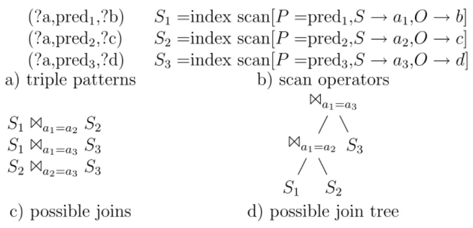
(?a,pred1,?b) (?a,pred2,?c) (?a,pred3,?d)

S1 =index scan[P =pred1,S →a1,O →b]

S2 =index scan[P =pred2,S →a2,O →c]

S3 =index scan[P =pred3,S →a3,O →d]

a) triple patterns b) scan operators

S1 1a1=a2 S2 S1 1a1=a3 S3 S2 1a2=a3 S3 1a1=a3 1a1=a2 S1 S2 S3

c) possible joins d) possible join tree

Figure 5.1: Example for reasoning using attribute equivalence classes multiple plans for a subgraph none of which dominates the other, all of them are kept in the DP table. This happens when good plans produce different output orders.

The optimizer seeds its DP table with scans for the base relations, in our case the triple patterns. The seeding is a two step process. First, the optimizer analyzes the query to check which variable bindings are used in other parts of the query. If a variable is unused, it can be projected away by using an aggregated index (see Section 3.3). Note that this projection conceptually preserves the cardinality through the count information in the index (see Subsection 4.3). In the second step the optimizer decides which of the applicable indexes to use. There are two factors that affect the index selection. When the literals in the triple pattern form the prefix of the index key, they are automatically handled by the range scan. Otherwise too many tuples are read and additional selections are required. On the other hand, a different index might produce the triples in an order suitable for a subsequent merge-join later on, which may have lower overall costs than reading too many tuples. The optimizer therefore generates plans for all indexes and uses the plan pruning mechanism to decide if some of them can be discarded early on.

Pruning the search space of possible execution plans is based on estimated execution costs. The optimizer calls the cost model for each generated plan and prunes equivalent plans that are dominated by cheaper alternatives. This pruning mechanism relies on order optimization [51] to decide if a plan is dominated by another plan. As the optimizer can use indexes on all triple permutations, it can produce tuples in an arbitrary order, which makes merge joins very attractive. Thus some plans are kept even if they are more expensive but produce an interesting ordering that can be used later on. Note that orderings are not only created by index scans but also by functional dependencies induced by selections; therefore the order optimization component is non-trivial [51]. We utilize the techniques of [36] for this purpose.

(26)

6-triples 8-triples 10-triples star patterns star patterns star patterns path length 5 0.7 ms 2.4 ms 6.4 ms path length 10 2.0 ms 4.6 ms 17.3 ms path length 20 3.5 ms 13.0 ms 56.6 ms

Figure 5.2: Optimization times for queries withx patterns in two stars connected by a path of lengthy

Starting with the seeds, larger plans are created by joining optimal solutions of smaller problems. During this process all attribute-handling logic for comparing values is implemented as reasoning over equivalence classes of variables instead of individual variable bindings. Variables that appear in different triple patterns are equivalent if they must have the same bindings to values in the final result of the query. These equivalence classes are determined at compile-time. It is sufficient that an execution plan produces at most one binding for each equivalence class (and no bindings for variables that do not appear in the query output). This simplifies implicit projections that precede pipeline breakers (e.g., hash-table build for a hash-join) and also allows for automatic detection of transitive join conditions (e.g.,a =b∧b=c⇒a=c).

An example for this reasoning is shown in Figure 5.1. It shows a query with three triple patterns (Figure 5.1 a) and joins on the common attributea between the patterns. The first translation step creates index scans for the three patterns (Figure 5.1 b), producing attributesa1,b, a2 ,c, a3, andd. Note that the ai are

really different from each other in terms of their value bindings; we named them similarly to show the connection to the original query variable. We can derive three join operators from the query graph (Figure 5.1 c), but in the final join tree (Figure 5.1 d) we use only two of them. The canonical translation would add another σa2=a3, but we can deduce that a1 and a2 are in the same equivalence

class, thus the 1a1=a3 is sufficient. Note that equivalence classes are derived from

equality conditions, not only from join-variable names. We could perform the same reasoning if the three patterns had no variable in common but instead joined via FILTER conditions.

Starting with the index scans seeds, larger plans are created by joining optimal solutions of smaller problems that are adjacent in the query graph [33]. When the query contains additional selections due toFILTER predicates, they are placed greedily as soon as possible, as they are usually inexpensive to evaluate. If a selection is really expensive, it could be better to integrate it into the DP operator placement as proposed in [10], but we did not investigate this further. The DP method that we implemented along these lines is very fast and is able to compute the exact cost-optimal solution for join queries with up to 20 triple patterns. We measured optimization times (in milliseconds) for a typical SPARQL scenario

(27)

with two entities selected by star-shaped subqueries and connected by a chain of join patterns. The results are shown in Figure 5.2. Note that the resulting plans are always optimal relative to the estimates by the cost model.

(28)

6 Selectivity Estimates

The query optimizer relies upon its cost model in finding the lowest-cost execution plan. In particular, estimated cardinalities (and thus selectivities) have a huge impact on plan generation. While this is a standard problem in database systems, the schema-free nature of RDF data complicates statistics generation. We propose two kinds of statistics. The first one, specialized histograms, is generic and can handle any kind of triple patterns and joins. Its disadvantage is that it assumes independence between predicates, which frequently does not hold in tightly coupled triple patterns. The second statistics therefore computes frequent join paths in the data, and gives more accurate predictions on these paths for large joins. During query optimization, we use the join-path cardinalities when available and otherwise assume independence and use the histograms.

6.1 Selectivity Histograms

While triples conceptually form a single table with three columns, histograms over the individual columns are not very useful as most query patterns touch at least two attributes of a triple. Instead we harness our aggregated indexes, which are perfectly suited for the calculation of triple-pattern selectivities: for each literal or literal pair, we can get the exact number of matching triples with one index lookup. Unfortunately this is not sufficient for estimating join selectivities. Also, we would like to keep all auxiliary structures for the cost model in main memory. Therefore, we aggregate the indexes even further such that each index fits into a single database page and includes information about join selectivity.

Just like the aggregated indexes we build six different statistics, one for each order of the entries in the triples. Starting from the aggregated indexes, we place all triples with the same prefix of length two in one bucket and then merge the smallest two neighboring buckets until the total histogram is small enough. This approximates an equi-depth histogram, but avoids placing bucket boundaries between triples with the same prefix (which are expected to be similar).

For each bucket we then compute the statistics shown in Figure 6.1. The first three values – the number of triples, number of distinct 2-prefixes, and number of

(29)

start end (s,p,o) (s,p,o) number of triples

number of distinct 2-prefixes number of distinct 1-prefixes join partners on subject

s=s s=p s=o join partners on predicate

p=s p=p p=o join partners on object

o=s o=p o=o

Figure 6.1: Structure of a histogram bucket

distinct 1-prefixes – are used to estimate the cardinality of a single triple pattern. Note that this only gives the scan cardinality, i.e., the number of scanned triples, which determines the costs of an index scan. The true result cardinality, which affects subsequent operators, could actually be lower when literals are not part of the index prefix and are tested by selections later on. In this case we derive the result cardinality (and obtain exact predictions) by reordering the literals such that all literals are in the prefix.

The next values are the numbers of join partners (i.e., the result cardinality) if the triples in the bucket were joined to all other triples in the database according to the specified join condition. As there are nine ways to combine attributes from two triples, we precompute nine cardinalities. For example the entry o = s is effectively

|{b|b∈current bucket}1b.object=t.subject {t|t∈all triples}|.

These values give a perfect join-size prediction when joining a pattern that exactly matches the bucket with a pattern without literals. Usually this is not the case, we therefore assume independence between query conditions and multiply the selectivities of the involved predicates. (Such independence assumptions are standard in state-of-the-art query optimizers for tractability.)

6.2 Frequent Paths

The histograms discussed above have decent accuracy, and are applicable for all kinds of predicates. Their main weakness is that they assume independence between predicates. Two kinds of correlated predicates commonly occur in SPARQL queries. First, “stars” of triple patterns, where a number of triple patterns with different predicates share the same subject. These are used to

(30)

select specific subjects (i.e., entities based on different attributes of the same entities). Second,“chains” of triple patterns, where the object of the first pattern is the subject of the next pattern, again with given predicates. These chains correspond to long join paths (across different entities). As both of these two cases are common, we additionally build specialized statistics to have more accurate estimators for such queries.

To this end, we precompute the frequent paths in the data graph and keep exact join statistics for them. Frequency here refers to paths with the same label sequence. Note that we use the term path both for chains and stars, the constructions are similar in the two cases. We characterize a path P by the sequence of predicatesp1, . . . , pn seen in its traversal. Using SPARQL syntax, we

define a (chain) path Pp1,...,pn as

Pp1,...,pn := select r1 rn+1 where { (r1 p1 r2). (r2 p2 r3). . . .(rn pn rn+1)}

Star paths are defined analogous, the p1, . . . , pn are unsorted in this case. We

compute the most frequent paths, i.e., the paths with the largest cardinalities, and materialize their result cardinalities and path descriptionsp1, . . . , pn. Using

this information we can exactly predict the join cardinality for the frequent paths that occur in a query. Again, we want to keep these statistics in main memory and therefore compute the most frequent paths such that they still fit on a single database page. In our experiments we could store about 1000 paths on one 16KB page.

Finding the most frequent paths requires some care. While it may seem that this is a standard graph-mining issue, the prevalent methods in that line of research [18, 60, 66], e.g., based on the well-known Apriori frequent-itemset mining algorithm, are not directly applicable.

Unlike the Apriori setting, a frequent path in our RDF-path sense does not necessarily consist of frequent subpaths. Consider a graph with two star-shaped link clusters where all end-nodes are connected to their respective star centers by predicates (edge labels) p1 and p2, respectively. Now consider a single edge with predicatep3 between the two star centers. In this scenario, the path Pp3 will be

infrequent, while the path Pp1,p3,p2 will be frequent. Therefore we cannot simply

use the Apriori algorithm.

Another problem in our RDF setting are cycles, which could lead to seemingly infinitely long, infinitely frequent paths. We solve this problem by two means. First, we require that if a frequent path P is to be kept, all of its subpaths have to be kept, too. This is required for query optimization purposes anyway, as we may have to break a long join-path into smaller joins, and it simplifies the frequent-path computation. Second, we rank the frequent paths not by their result cardinalities but by their number of distinct nodes. In a tree these two are identical, but in the presence of cycles we do not count nodes twice.

The pseudo-code of the path mining algorithm is shown in Figure 6.2. It starts from frequent paths of length one and enlarges them by appending or prepending

(31)

FrequentPath(k)

// Computes thek most frequent paths

C1 ={Pp|p is a predicate in the database}

sort C1, keep the k most frequent

C=C1,i= 1

do

Ci+1 =∅

for each p0 ∈Ci, p predicate in the database

iftop k of C∪Ci+1∪ {Pp0_p}includes all subpaths of p0p

Ci+1 =Ci+1∪ {Pp0_p}

iftop k of C∪Ci+1∪ {Ppp0}includes all subpaths of pp0

Ci+1 =Ci+1∪ {Ppp0}

C =C∪Ci+1, sort C, keep the k most frequent

Ci+1 =Ci+1∩C, i=i+ 1

while Ci 6=∅

returnC

Figure 6.2: Frequent Path Mining Algorithm

predicates. When a new path is itself frequent and all of its subpaths are still kept, we add it. We stop when no new paths can be added. Note that, although the pseudo-code shows a nested loop for ease of presentation, we actually use a join and a group-by operator in the implementation. For the datasets we considered in our experiments the 1000 most frequent paths could be determined in a few minutes.

6.3 Estimates for Composite Queries

For estimating the overall selectivity of an entire composite query, we combine the histograms with the frequent paths statistics. A long join chain with intermediate nodes that have triple patterns with object literals is decomposed into subchains of maximal lengths such that only their end nodes have triple patterns with literals. For example, a query like

?x1 a1 v1. ?x1 p1 ?x2. ?x2 p2 ?x3. ?x3 p3 ?x4. ?x4 a4 v4. ?x4 p4 ?x5. ?x5 p5 ?x6. ?x6 a6 v6

with attribute-flavored predicates a1, a4, a6, literals v1, v4,v6, and relationship-flavored predicates p1 through p5 will be broken down into the subchains for

p1-p2-p3 and for p4-p5 and the per-subject selections a1-v1, a4-v4, and a6-v6. We use the frequent paths statistics to estimate the selectivity of the two join subchains, and the histograms for selections. Then, in the absence of any other statistics, we assume that the different estimators are probabilistically independent, leading to

(32)

a product formula with the per-subchain and per-selection estimates as factors. If instead of a simple attribute-value selection like ?x6 a6 v6 we had a star pattern such as ?x6 a6 u6. ?x6 b6 v6. ?x6 c6 w6 with propertiesa6,b6,c6 and corresponding object literals u6, v6, w6, we would first invoke the estimator for the star pattern, using the frequent paths statistics for stars, and then combine them with the other estimates in the product form.

(33)

7 Managing Updates

So far we have solely considered static RDF databases that are bulk-loaded once and then repeatedly queried. The current RDF and SPARQ standards [41, 52] do not discuss any update operations, but an RDF database should support data changes and incremental loading as well.

In designing the management of updates for RDF-3X, we make the following assumptions about typical usage patterns:

1. Queries are far more frequent than updates, and also much more resource consuming.

2. Updates are mostly insertions of new triples. Overwriting existing triples (updates-in-place) are rarely needed; rather new versions and annotations would be created.

3. Updates can usually be batched, boiling down to incremental loading. 4. It is desirable that (batched) updates can be performed concurrently with

queries, but there is no need for full-fledged ACID transactions.

Based on these assumptions, we have designed and implemented a differential indexingmethod for RDF-3X that supports both individual update operations and entire batches. The key idea is that updates are initially applied to small differential indexes, deferring the actual updates to the main indexes. The differential indexes can be easily integrated into the query processor, and are thus transparent to application programs. Periodically or after reaching a certain size, differential indexes are merged into the main indexes in a batched manner. This overall architecture for managing updates in RDF-3X is illustrated in Figure 7.1. In Subsections 7.1 and 7.2 we first discuss the insertion of new triples, introduc-ing our additional data structures, and the deletion of existintroduc-ing triples. Updates to existing triples, if ever needed, must be expressed as a pairs of deletions and insertions. Although full ACID transactions are beyond our current scope, we do provide rudimentary support for atomic batches of operations. This will be discussed in Subsection 7.3.

(34)

Main Indexes Differential Indexes Queries Updates S P O Dict2 Batched Merges

Dict1 _Dict1Dict2

SP SO PS PO OS OP SPO SOP PSO POS OSP OPS SPO SOP PSO POS OSP OPS

(35)

7.1 Insert Operations

Inserting new triples into a database is a performance challenge because of the aggressive indexing on which RDF-3X is based. In principle, the indexes can be easily updated as they are standard B+-trees, but each new triple would incur access to 15 indexes. Furthermore, the updates are computationally more expensive than usual due to the compressed leaf pages. This makes direct updates to indexes unattractive.

To avoid these costs, we use astaging architecturewith deferred index updates. All updates are first collected in workspaces, and all their triples are indexed separately from the main database in differential indexes. Periodically, or when the size of the differential indexes exceeds a specified limit, all staged changes are integrated into the main indexes described in Section 3. During query processing, the query compiler adds additional merge joins with the, usually very small, differential indexes to transparently integrate deferred updates if they satisfy query conditions. The principles of this architecture resemble the rationale of the multi-component LSM-tree [38] and similar data structures with batched updates such as [15, 35, 27, 47]. In the following we present more details on 1) workspace management, 2) differential indexes, 3) extended query processing.

Workspace Management. Each application program that interacts with the

RDF-3X engine has a private workspace in memory. We expect that the following is the most typical update pattern: a program loads a new RDF file into the database, generating a large number of new triples without any queries. Additionally but much less frequently, programs can mix updates and queries, deriving new triples from existing ones. But in this case, we expect that the number of generated triples is much smaller.

With consideration to these two usage patterns, we index the new triples lazily. Initially we just store them in an in-memory heap as they arrive. Only when we need a certain triple ordering for query processing, we generate the desired index by sorting the triples in the workspace. For programs that interleave queries and updates, we expect bursts of insertions (i.e., many new triples derived from a query result). Therefore, we do not maintain the indexes but simply invalidate the indexes after a new update and rebuild them from scratch when needed for a later query. When the program terminates (or at a program-specified “commit point”, see below), we build indexes for all six triple orderings and merge them into the corresponding differential indexes that are shared across all programs. In addition, the workspace manager for each program also maintains a string dictionary for new strings. We generate temporary string ids for each program, which are later resolved into final ids during the merge with the differential index. This technique avoids the need for concurrency control on the globally shared string dictionary, and is safe as the ids are not visible at the application level.

Differential Indexes. The differential indexes, which are shared by all programs, are an intermediate layer between the programs’ private workspaces and the

(36)

full indexes of the main database. This intermediate indexing allows us to improve update throughput by aggregating many new triples into bulk operations against the main indexes. We keep differential indexes in main memory in our implementation, which simplifies their maintenance. When they exhaust a given memory budget, we initiate a merge process into the main indexes to release memory. For recoverability after soft crashes that lose memory content, newly created triples are written to a disk-resident log file in their plain form (i.e., only once, not in six different orders). Alternatively, we could store the differential indexes in flash RAM.

The differential indexes are B+-trees for the different triple orderings, similarly to the main indexes of Section 3. However, there are some differences. First, we only build the six full indexes for the different attribute permutations; there is no need for building the binary or unary aggregation indexes. As all data is in main memory, we can inexpensively construct aggregated indexes on the fly when needed, by using sort-based group-by operators. Furthermore, the indexes are not compressed, as we want to be able to modify them as fast as possible. Finally, we use a read-copy-update (RCU) mechanism [21] to allow queries to perform scans on the differential indexes without any concurrency control. This is similar to Blink-tree-style techniques [30] but simpler and not as powerful. When a tree page is modified, we first copy the page, modify the page, and then change all pointers to the old page to point to the new page. Note that this only maximizes concurrency for read operations; write operations on the tree have to latch pages to protect the tree from becoming inconsistent because of concurrent writers. Further note that while the RCU mechanism allows for concurrent operations, it does not provide transaction isolation. Similarly to the workspace management, the differential index management also includes maintaining a string dictionary for new strings, but here the string ids are already the final ones that will later be used in the disk-resident main indexes. The string dictionary also uses an RCU mechanism to allow lock-free reads, so queries are never blocked.

Merging the six differential indexes into the corresponding main indexes of the database is I/O-intensive and thus expensive, but relatively simple. Some care is needed because of the compression in the main indexes, but as compressed pages are self-contained and never need any other pages for uncompression, we can perform the merge page by page. Each of the six index merges can be performed independently. Overall, the merge process works pretty much like a standard bulk insertion of sorted data into a B+_-tree.

The string dictionary of the main database is updated as well, but here the merging is even simpler because of the absence of compression and the monotonicity of string ids (which means that without deletions new entries are always appended).

(37)

differential indexes, and the workspace of the program that invokes the query:

SP Oquery=SP O∪SP Odif f ∪SP Oprog

As all three indexes are sorted in the same way, we use merge-joins with union semantics (1merge∪ ) to combine the indexes. For example the triple pattern

(90,?a,?b) would be translated into the following expression: (σS=90(SP O)) 1∪merge (σS=90(SP Odif f))

1merge

∪ (σS=90(SP Oprog))

These join operators are very cheap and require no additional memory, but cause some small CPU overhead due to additional comparisons. This is slightly troublesome, as each triple pattern in a query generates two of these extra joins. Most of these joins will turn out to be unnecessary, namely, whenever there are no new triples in the differential indexes or workspace that match a given triple pattern. The RDF-3X system therefore tries to eliminate unnecessary joins of this kind. One way to detect unnecessary scans of the differential indexes is to check for relevant triples during query compilation, as the differential indexes are in main memory anyway. Unfortunately, this approach faces complications when queries contain selections that are pushed down below joins by the query optimizer. Instead, we implemented the1merge∪ operator such that at query execution time

it removes itself from the execution plan once one of its inputs (differential index or workspace) is or becomes empty.

7.2 Delete Operations

The algorithms for handling deletions and for running queries in the presence of deletions are very similar to the described case of insertions. When deleting a triple, we “insert” the triple into the workspace and differential indexes with a deletion flag. During queries, the 1merge∪ operator interprets this flag and behaves

like an anti-join when encountering deleted triples, eliminating matching triples on the other side. When merging the differential indexes into the main indexes, triples marked for deletion cause the deletion of their counterparts in the main indexes and are discarded after the entire merge completes.

While deleting the triples themselves is simple, maintaining a compact string dictionary is more challenging. Ideally we want to eliminate strings that are no longer referenced by any triple, to avoid monotonic growth of the dictionary. When deleting a single triple we do not know a priori if the strings used by the triple occur in any other triples. We can find this out by checking the fully aggregated indexes of RDF-3X, which implicitly give the number of occurrences for each string, but checking these for each triple would be expensive. Fortunately we do not have to check for each triple, but only when we eliminate an entry

(38)

from an aggregated unary index. Assume that we want to delete the SPO triples (1,2,3) and (1,4,5). When merging the corresponding differential index entries into the main indexes, the aggregated unary index for S will be looked up with value S= 1. The count entry for 1 is decreased by two to reflect two eliminated triples. Only if the count reaches zero the whole entry is eliminated, and only in this case do we check if the value 1 occurs in the other two unary indexes forP

andO. If none of the unary indexes signals the presence of the value 1, we can remove 1 from the dictionary.

Alternatively to the immediate checking of all unary indexes, we could periodi-cally run a garbage collector to eliminate strings with zero references. This can be implemented by a single merge scan over the three unary aggregation indexes and the string dictionary. It depends on the data and the update behavior whether this is more efficient or not. If we assume that deletions are very infrequent, it is cheaper to perform the checks immediately as described above.

7.3 Support for Atomicity and Weak Isolation

The above procedures provide proper isolation between individual operations, but no transactional ACID guarantees for entire blocks of operations. While full-fledged transactions are beyond the scope of this paper, we have successfully added support for the atomicity of programs and a weak form of isolation level among concurrent program executions.

In the first stage of our staging architecture, programs that contain only update operations (and no queries) are automatically isolated by using their private workspaces. A program’s termination can thus be easily viewed as a “commit point”. Alternatively, a program can specify multiple commit points during its run-time; each commit point prompts a merge with the globally shared differential indexes. During merges with the differential indexes and with the main indexes, the consistency of the index trees is guaranteed by latching and the RCU mechanism. When a program merges its workspace into a differential index, it latches index leaf pages in a lock-coupling manner, always holding latches for two successive leaf pages at the same time. As all write programs have the very same page access order during such a merge, the lock-coupling technique guarantees serializability between such write-only programs. The merges are naturally idempotent, so we obtain crash-resilience for free: an interrupted merge can simply be restarted and would then ignore inserted triples that are already present in the merge target.

Programs that issue only queries can run against both the differential indexes and the main indexes without any locking or latching (even the latter is avoided because of the RCU mechanism for concurrent writers). Of course, it is impossible to guarantee transactional serializability between readers and writers this way, and even snapshot isolation is not feasible this way. However, no query will

(39)

ever see a non-committed update, as merges from workspaces into differential indexes start only after commit points. Thus, our staging architecture provides theread-committed isolation level, which seems sufficient for many applications outside enterprise-business IT. This property also holds for programs that mix queries and updates: all their queries see committed data and their updates are properly serialized against concurrent read-write programs.

Overall, the deferred update handling has the following salient properties: 1. Query execution times are unaffected if there are no updates that satisfy

any triple patterns in the query, and have very small overhead otherwise. 2. Updates to the main indexes are aggregated into efficient bulk operations. 3. We provide support for atomic batches of update operations. Queries never have to wait; they run at the read-committed isolation level (which is weaker than serializability or snapshot isolation).