Departamento de Economía
Ekonomia Saila
Documentos de Trabajo
Lan Gaiak
ESTIMATION OF THE COINTEGRATING RANK IN
FRACTIONAL COINTEGRATION
Javier Hualde
D.T. 1205
Estimation of the cointegrating rank in
fractional cointegration
∗
Javier Hualde
Universidad Pública de Navarra
August 9, 2012
Abstract
This paper proposes an estimator of the cointegrating rank of a po-tentially cointegrated multivariate fractional process. Our setting is very flexible, allowing the individual observable processes to have different in-tegration orders. The proposed method is automatic and can be also em-ployed to infer the dimensions of possible cointegrating subspaces, which are characterized by special directions in the cointegrating space which gen-erate cointegrating errors with smaller integration orders, increasing the “achievement” of the cointegration analysis. A Monte Carlo experiment of finite sample performance and an empirical analysis are included.
JEL Classification: C32.
Keywords. Fractional integration; cointegrating rank; cointegrating space and subspaces.
∗Thanks to Søren Johansen for useful comments. This research is supported by the Spanish
1. INTRODUCTION
Since the seminal paper of Engle and Granger (1987), the concept of coin-tegration has been generalized in several directions. One of the most recent developments is that of fractional cointegration, where, unlike in the standard setting of unit root observables with weak dependent cointegrating errors, series are allowed to have fractional integration orders. This generalization captures in-teresting possibilities, like that of nonstationary but mean reverting cointegration errors (with applications in macroeconomics), or stationary cointegration, where the observables are stationary (but long memory) with “less-memoried” (even short memory) cointegrating errors, with applications in finance (see Gil-Alana and Hualde, 2009, for a review).
However, even if theoretical developments have been numerous, it is not clear the extent to which they are influencing the empirical literature, possibly due to the absence of a feasible and general methodology. In particular, even if most studies impose that all observables share the same integration order (Kim and Phillips, 2000, Hurvich and Chen, 2006), it seems natural to think that this re-striction does not apply in practice. Then, a complicated cointegrating structure might occur, and issues like determining the cointegrating rank r (the dimen-sion of the cointegrating space), which is necessary in order to make inference on cointegrating vectors, are far from being trivial. In fact, methodologies for esti-mating the rank, as the ones proposed by Robinson and Yajima (2002) or Robin-son (2008), are not designed to cover all cases where observables have distinct integration orders. Thus, our purpose in the present paper will be to propose an automatic method to infer r which does not require any prior information about memory or cointegrating characteristics of the observables. Incidentally, our method offers two additional advantages. First, it leads to straightforward estimation of the cointegrating space. Second, our methodology could be also used to uncover the dimension of possible cointegrating subspaces (special direc-tions in the cointegrating space which generate cointegrating errors with smaller integration orders), and estimate them by simple methods. In this sense, our procedure could be viewed as an alternative to Chen and Hurvich (2006), al-though they assume that all observables share the same memory parameter and, in addition, our approach is much closer to the simultaneous equations model methodology, with very long tradition in econometrics.
The plan of the paper is as follows. In Section 2 we propose an estimator of the dimension of the cointegrating space and give guidance on how to estimate it. Next, in Section 3, we present a Monte Carlo experiment of finite sample performance. In Section 4 we apply our method to a trivariate series of oil prices, and illustrate the issue of estimating a cointegrating subspace. Finally, in Section 5, we conclude. All proofs are relegated to the Appendix.
2. ESTIMATION OF THE COINTEGRATING RANK
First, we model a p×1 vector of observables zt. Let ut be a p-dimensional
covariance stationary process with spectral density positive definite and bounded at all frequencies; for real numbers θi, i = 1, ..., p, such that θi < 1/2, define
st = diag∆−θ1, ...,∆−θput, where ∆ = 1−L, L being the lag operator.
De-note by ait the ith component of an arbitrary vector at. Then sit ∼ I(θi),
where I(d) stands for Type I fractionally integrated process of order d (see, e.g., Gil-Alana and Hualde, 2009). Let qi ∈ {0,1,2, ...}, i = 1, ..., p. Define
vt=diag(∆−q1, ...,∆−qp){st1 (t >0)}, where1 (·)is the indicator function (this
implies fixing initial conditions to zero, but our results are identical for initial conditions fixed in alternative ways). Letδi =θi+qi. Thenvit ∼I(δi), which is
covariance stationary ifqi = 0, or built on partial sums of a covariance stationary
process if qi > 0. Without loss of generality (apart from not allowing negative
memories), set 0≤ δ1 ≤δ2 ≤ ...≤ δp, with also δp >0. Let the p×1 vector of
observableszt be generated by
Υzt=vt,t = 1,2, ..., (1)
where Υ is nonsingular. Then, zt = Υ−1vt, so the variables in zt are modelled
as linear combinations of fractional processes (hence, inheriting, in general, the maximum of their integration orders). Model (1) appears to be a natural setting to discuss the possibility of cointegration, which throughout will refer to the situ-ation where a linear combinsitu-ation of fractional processes is integrated of a strictly smaller order than the maximum order of the elements of the linear combina-tion. This definition covers many situations. For example, if one of the variables has an integration order strictly larger than the rest of the variables, any linear combination which puts zero weight on this particular variable is considered to be a (trivial) cointegrating relation. The definition is similar to that of Johansen (1995), and more general than those of Flores and Szafarz (1996), Marinucci and
Robinson (2001) and Robinson and Yajima (2002). When all variables enjoy the same integration order, all different definitions coincide, being also identical to the original one given in Engle and Granger (1987).
Related to (1), the nonsingularity ofΥand the assumptions onut(so
nontriv-ial cointegration cannot occur among the elements ofvt), imply that at least one
of the elements ofztisI(δp), although the possibility that all variables inztshare
the same integration order is also captured if the last column ofΥ−1 contains no
zeroes. In generalzit ∼I(di), i= 1, ..., p, where the linkage between the di’s and
theδi’s depends on Υ. Note that by (1), zt might be subject to a very
compli-cated cointegrating structure (depending both on restrictions inΥ, which might eliminate trends in certain linear combinations, and strict inequalities among the
δi’s)
The main aim of the paper is to propose an estimator of the cointegrating rank ofzt. Our methodology will be based on applying sequentially the following
theorem. We do not give its proof, as it is just Theorem 2 of Gomez-Biscarri and Hualde (2011) applied to our fractional setting. Denote by “common trends”
I(δp) and noncointegrated variables.
Theorem 1. zt in (1) has cointegrating rank r ∈ {1, ..., p−1} if and only if a.
and b. hold, where: a. There exists a (p−r)-dimensional subvector of zt (say
z(b)t), whose individual components are common trends; b. All subvectors of zt
of dimension larger thanp−r containing z(b)t cointegrate.
The implementation of our procedure is based on estimators of the individual integration orders (di,i= 1, ..., p) and test statistics (τj1,...,jk) for
Hj1,...,jk :{zj1t, zj2t, ..., zjkt are not cointegrated};Hj1,...,jk :Hj1,...,jk is not true,
where j1, ..., jk ∈ {1, ..., p}, k ≤ p. Let g1n be the rate of convergence of the
di’s, and g2n be the rate of divergence under the alternative of the τj1,...,jk’s (if
it is different for the various test statistics, take g2n as the minimum of the
rates). Also, assume that τj1,...,jk has asymptotic size α. Possible choices for
di are the log-periodogram (Robinson, 1995a) or the local Whittle (Robinson,
1995b) estimators, for whichg1n=m1/2, wheremdenotes bandwidth. Regarding
τj1,...,jk, Robinson (2008) (whereg2n =m) or Hualde and Velasco (2008) (where
g2n depends on a complicated manner on the integration orders involved,m and
orders of the observables. Lethn >0 be a sequence (whose role will be clarified
in Theorem 2 and Remark 1 below) such that
hn+ (g1n+g2n)h−n1 → ∞as n→ ∞. (2)
The steps characterizing our procedure are as follows:
Step 1. Estimate di by di, i = 1, ..., p. Then choose a possible common trend
variable zc1t, c1 ∈ {1, ..., p}. In particular, choose c1 =pif g1n(dp−di)> hn, for
all i = 1, ..., p−1; otherwise, choose c1 = p−j if g1n(dp−j −di) > hn, for all
i = 1, ..., p−j −1, checking these conditions sequentially for j = 1, ..., p−2; if none of these conditions is fulfilled, choosec1 = 1. Note that there is a particular
ordering in our choice, but the limiting properties of our proposed estimator ofr
are invariant to it. Next, reorder the variables inzt so that zpt =zc1t in the new
ordering (this reordering is irrelevant for the results, but simplifies subsequent notation substantially). Then, given the possible common trend zpt, we test for
H(1) : ∪pi=1−1Hp,i, H(1) : ∩ip=1−1Hp,i, and set {r=p−1} = {H(1) is rejected}.
Note that if zpt ∼ I(δp), then by Theorem 1, H(1), H(1) are equivalent to
r < p−1, r=p−1, respectively, which justifies r.
Step 2. If H(1) is not rejected, choose zc2t, c2 ∈ {1, ..., p−1} so the possible
common trends are zpt, zc2t. In particular, choose c2 =p−1if τp,i−τp,p−1 > hn
for all i = 1, ..., p−2; otherwise, choose c2 = p−j if τp,i−τp,p−j > hn for all
i= 1, ..., p−j−1, checking these conditions sequentially forj = 2, ..., p−2; if none of these conditions is fulfilled, choosec2 = 1. Reorder again the variables so that
zpt =zc1t, zp−1,t =zc2tin the new ordering. Then we test forH(2) :∪ p−2
i=1Hp,p−1,i,
H(2) :∩pi=1−2Hp,p−1,i, and estimate the rank by
{r=p−2}={H(1) is not rejected and H(2) is rejected}.
Note that ifzpt,zp−1,t are valid common trends, thenH(1)∩H(2),H(1)∩H(2)
are equivalent tor < p−2, r=p−2, respectively, which justifies r.
In general, fork = 2, ..., p−1, we have
Step k. If H(k−1) is not rejected, choose ck. Note that in previous steps
the variables have been reordered so that zpt = zc1t, ..., zp−k+2,t = zck−1,t. Then
choose ck = p−k+ 1 if τp,...,p−k+2,i−τp,...,p−k+2,p−k+1 > hn for all i = 1, ..., p−
i = 1, ..., p − j − 1, checking these conditions sequentially for j = k, ..., p −
2; if none of these conditions is fulfilled, choose ck = 1. Reorder the
vari-ables so zpt = zc1t, ..., zp−k+2,t = zck−1,t, zp−k+1,t = zckt. Then test for H(k) : ∪pi=1−kHp,p−1,...,p−k+1,i, H(k) :∩pi=1−kHp,p−1,...,p−k+1,i, and set
{r=p−k}={H(i), i= 1, ..., k−1, are not rejected and H(k) is rejected},
and for the stepk =p−1, also{r= 0}={H(i), i= 1, ..., p−1, are not rejected}.
Before analyzing the properties of r, we derive a result concerning our choice of common trends. We introduce first some additional notation. Given the initial arbitrary ordering of the variables, let i1 ∈ {1, ..., p} be such that: zi1t ∼ I(δp);
i1 ≤l for any l such that zlt∼I(δp). Similarly, given the ordering ofzt afterc1
has been chosen (so zpt = zc1t), let i2 ∈ {1, ..., p−1} be such that: zpt and zi2t
are not cointegrated;i2 ≤l for anyl such thatzptandzltare not cointegrated. In
general, forj = 2, ..., p−1, letij ∈ {1, ..., p−j + 1}be such that: zpt, ..., zp−j+2,t
andzijt are not cointegrated;ij ≤l for any l such that zpt, ..., zp−j+2,tandzlt are
not cointegrated. Note that the existence of the ij’s depends onr. In particular,
if r = p−1, just i1 exists; if r = p− 2, just i1 and i2 exist; in general, for
r∈ {1, ..., p−1}, justi1, i2, ..., ip−r exist.
Theorem 2. Letr∈ {1, ..., p−1}be the cointegrating rank and (2) hold. Then, for any 1≤k ≤p−r, Pr (c1 =i1, c2 =i2, ...., ck =ik)→1 as n→ ∞.
Remark 1. Theorem 2 implies that, by usinghnsuch that (2) holds, we choose in
every step a single set of valid common trends with probability approaching one. Alternatively, it would be more natural to set hn = 0, because this implies that
zc1tis the variable with highest estimated order, zc2twould be the variable which
shows less evidence of being cointegrated withzc1t, and so on. However, in this
case, alternative sets of valid common trends could be chosen with nonnegligible (as n → ∞) probabilities (unlike in our setting, where just a particular set of valid common trends has a nonnegligible probability of being chosen), and this leads to a size control problem. Using hn satisfying (2) implies a unique choice
of valid common trends (asymptotically), and this allows us to control the size of our sequential method and derive the neat results (3), (4), (5), (6) below. In practice, however, there is always a choice forhn as close to zero as desired, while
satisfying (2) (as the one we employ in the Monte Carlo experiment). The properties of r are given in the next theorem.
Theorem 3. Letr be the cointegrating rank and (2) hold. Then, asn→ ∞,
Pr (r=j) → 0, j = 0, ..., r−1, (3)
Pr (r=j) ≤ φn→α, j =r+ 1, ..., p−1, (4)
Pr (r=r) → 1, r=p−1, (5)
Pr (r=r) ≥ θn →1−(p−1−r)α, r < p−1. (6)
Remark 2. Results in Theorem 3 are identical to those corresponding to an alternative (infeasible) estimator ofr which bases every step of the procedure on true common trends. The reason is that, in every step, our method leads to valid common trends with probability tending to one.
Remark 3. Results in Theorem 3 are comparable to those of Theorem 12.3 of Johansen (1995) derived for standard cointegration, although there are a couple of differences. First, (5) is better than Johansen’s result (who obtained the limit
1−α). However, for r < p−1we obtained for Pr (r =r)a smaller lower bound than that achieved by Johansen (1−α). Nevertheless, note that the bound in (6) might not be strict and fits naturally with the upper bound given in (4).
Remark 4. Our procedure leads to straightforward estimation of the coin-tegrating space. In particular, suppose that the procedure is finalized in step
k, k = 1, ..., p −1, so r = p− k. This step determines that the variables in
z(b)t= (zpt, zp−1,t, ..., zp−k+1,t)′ are possible common trends (valid ones with
prob-ability approaching one). Collect the rest of the elements of zt inz(a)t. Theorem
1 ensures that if r=p−k and the elements ofz(b)t are common trends, any set
of k+ 1 variables formed by any of the variables in z(a)t and all those in z(b)t is
always cointegrated. Thus there exists ar×kmatrixB such that the components of z(a)t−Bz(b)t have integration orders smaller than δp. B can be estimated by
standard methods like ordinary least squares (OLS) or narrow band least squares (NBLS), the components in z(a)t being dependent variables and z(b)t the vector
of regressors. NBLS provides consistent estimators in all situations.
Remark 5. Our procedure can be used to infer the dimension of possible cointe-grating subspaces. In fact, it can be shown that the dimension of a cointecointe-grating subspace can be inferred by applying our method to a set of cointegrating er-rors. The obvious difficulty is that those errors are unknown, although, they can be proxied by residuals. Then, the crucial issue is to justify that the
inferen-tial procedures employed (di andτj1,...,jk) retain their properties when applied to
residuals. A proper justification of this depends on the precise inference methods employed and goes beyond the scope of the present paper, although results in Hualde and Robinson (2006) indicate that this might be the case in many cir-cumstances. We illustrate in Section 4 the problem of inferring the dimension of a cointegrating subspace and its estimation by means of a simple empirical example.
3. MONTE CARLO EVIDENCE
We investigate the finite sample performance of r by means of a Monte Carlo experiment. Our analysis is based on 5000 replications of three series
zit, i = 1,2,3, of lengths n = 256,512, generated according to five
differ-ent DGP’s, the numbering indicating the cointegrating rank (in all cases the
ut below are independent trivariate normal vectors such that V ar(uit) = 1,
i = 1,2,3, Cov(uit, ujt) = 0.5, i = j): 0) zit = ∆−.35uit, i = 1,2,3; 1a)
zit= ∆−.35uit, i= 1,2,z3t=u3t; 1b) zit = ∆−.35uit, i= 1,2,z3t+z2t−z1t=u3t;
2a) z1t = ∆−.35u1t, zit = uit, i = 2,3; 2b) z1t = ∆−.35u1t, z2t − z1t = u2t,
z3t−z2t−z1t=u3t. Note that the a) cases reflect the situation where thezithave
distinct integration orders, whereas under b), the zit share the same integration
order, but they are cointegrated. In all cases the maximum integration order of the observables is 0.35, whereas cointegrating errors are always weak dependent. The fractional processes were generated by the algorithm designed by Davies and Harte (1987). We implement our procedure by using local Whittle estimation of the orders (Robinson, 1995b) and we test forHj1,...,jk by the Υ
∗
m semiparametric
test statistic of Hualde and Velasco (2008) (using sizes α = .10, .05, .01), zjkt
taking the role of theyt variable in Hualde and Velasco’s notation (this statistic
is designed to be applied to Type II fractional processes, but it can be shown to be also adequate for Type I). Given that our inferential procedures are semipara-metric, to check sensibility to bandwidth choice, we give results for m = 55,80
and m = 100,150, for n = 256,512, respectively. We set hn = log(m10
−13 ), so effectively hn is indistinguishable from zero, while satisfying (2). We present in
Table 1 the proportion of replications leading to each r in the five different sce-narios. Given the very adverse situation we face (with very small cointegrating gaps), our procedure, which is favoured when the cointegration is not trivial, per-forms very satisfactorily, especially for r= 2 as (5) suggests. In few cases r = 0
is chosen too frequently, but more often r > r occurs, because our test statistic is usually oversized. However results improve substantially as n andm increase (note that given our design, we approach a parametric procedure asm→n/2).
4. EMPIRICAL EXAMPLE
We apply our procedure to a trivariate series of 381 monthly observations (from January 1980 through September 2011) on Dubai, Brent, and West Texas Intermediate (WTI) oil prices (in $ per barrel) collected from the IMF Primary Commodity Prices database. We analyse log prices and identify Dubai, Brent and WTI log prices with z1t, z2t and z3t, respectively. Similar data (for a much
shorter time span) was employed in the empirical analysis of Robinson and Ya-jima (2002).
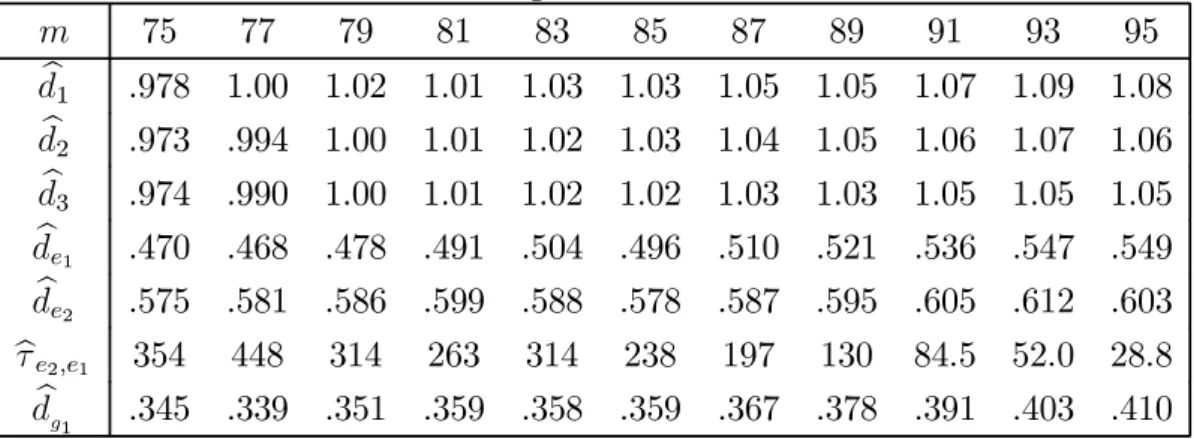
First, we estimate the integration orders of zit by local Whittle. Given that
nominal price series are usually characterised by strong nonstationarity (being this also confirmed by a preliminary graphical analysis), we use in our estimation first differences of the series. Estimates of the orders (adding back one to the values obtained from the differenced series) for bandwidth choicesm= 75+2i,i= 0,1, ...,10, are reported in Table 2. Unlike the estimates presented by Robinson and Yajima (2002) (whose values were around 0.5), ours are in all cases very close to one. We also computed results for smaller bandwidths (m ≥ 15), and in all cases the estimates were larger than 0.75 (most of them were between 0.8 and 1). Any of our bandwidth choices led to the identification of the common trend as c1 = 1. Based on this, we computed Hualde and Velasco’s (2008) test
statistics τ1,2 and τ1,3, which in all cases took values much larger than critical
ones,τ1,2 being always larger thanτ1,3 (we do not report these statistics as they
are not very informative). Thus, we concluded r = 2, being this conclusion also supported by any choice of m ≥ 15. The cointegrating space was estimated by NBLS (with m = 85, although results are almost invariant to m) as the span of vectorsa1 = (−.967,1,0)′,a2 = (−.905,0,1)′.
In Table 2, we also report results concerning the identification of a possible cointegrating subspace. In particular, e1t, e2t refer to cointegrating errors from
the WTI-Dubai and Brent-Dubai cointegrating relations, respectively (proxied by NBLS residuals, eit, i= 1,2). Based on these residuals, we estimate by local
Whittle the memory of e1t, e2t (and present these estimates in Table 2), both
trend, we computed Hualde and Velasco’s (2008) test statistic (reported in Table 2 as τe2,e1) to asses whether those errors are cointegrated, and it appears to be
clearly the case, so, for our choices of m, the data support the existence of a cointegrating subspace. Note that dg1 reported in Table 2 is the local Whittle
estimate of the memory of this subspace (computed from residuals of the NBLS regression ofe1t one2t), being smaller than the estimated memories of e1t or e2t.
Our conclusion is robust to other choices ofmsuch thatm ≥75, whereas results for smallermindicate, in general, that cointegration between cointegrating errors is trivial. In any case, given that e1t =z3t−β31z1t, e2t =z2t−β21z1t, ife1t and
e2t are cointegrated, there exists θ such that z3t −β31z1t−θ(z2t−β21z1t) has
reduced order. Then this subspace can be easily estimated by NBLS, choosing
z3t as dependent variable and z1t, z2t, as regressors. Choosing m = 85, we
perform this estimation, concluding that the estimated subspace is the span of
b = (.078,−1.017,1)′. This estimate looks sensible becauseb is almost identical toa2−1.017a1, the very small estimated coefficient corresponding toz1t (0.078)
implying that the cointegration between Brent and WTI possibly leads to a smaller memory than the one between any other pair of observable series.
5. CONCLUSION
We have proposed an automatic method to infer the cointegrating rank which does not rely on previous knowledge of memory or cointegrating characteristics of the vector of observables. The procedure can be applied irrespective of the cointegrating structure of the observables, it performs well in finite samples and it leads to straightforward estimation of the cointegrating space. Our method can be also employed to estimate possible cointegrating subspaces, and we illustrated this possibility by means of a simple empirical example.
REFERENCES
Chen, W. & C.M. Hurvich (2006) Semiparametric estimation of fractional coin-tegrating subspaces. Annals of Statistics 27, 2939-2979.
Davies, R.B. & D.S. Harte (1987) Test for Hurst effect. Biometrika 74, 95-101. Engle, R.F. & C.W.J. Granger (1987) Cointegration and error correction model.
Representation, estimation and testing. Econometrica 55, 251-276.
Flores, R. & A. Szafarz (1996) An enlarged definition of cointegration.
Gil-Alana, L.A. & J. Hualde (2009) Fractional integration and cointegration: an overview and an empirical application. Palgrave Handbook of Econometrics, Vol. 2, Applied Econometrics (K. Patterson and T.C. Mills, eds.). Palgrave, MacMillan, pp. 434-469.
Gomez-Biscarri, J. & J. Hualde (2011) Regression-based identification and es-timation of cointegration structures. Preprint, Universidad Pública de Navarra.
Hualde, J. & P.M. Robinson (2006) Semiparametric estimation of fractional cointegration. STICERD Discussion paper EM/2006/502.
Hualde, J. & C. Velasco (2008) Distribution-free tests of fractional cointegration.
Econometric Theory 24, 216-255.
Johansen, S. (1995)Likelihood based inference in cointegrated vector autoregres-sive models. Oxford University Press.
Kim, S.C. & P.C.B. Phillips (2000) Fully modified estimation of fractional coin-tegration models. Preprint, Yale University.
Marinucci, D. & P.M. Robinson (2001) Semiparametric fractional cointegration analysis. Journal of Econometrics 105, 225-247.
Robinson, P.M. (1995a) Log-periodogram regression of time series with long range dependence. Annals of Statistics 23, 1048-1072.
Robinson, P.M. (1995b) Gaussian semiparametric estimation of long-range de-pendence. Annals of Statistics 23, 1630-1661.
Robinson, P.M. (2008) Diagnostic testing for cointegration. Journal of Econo-metrics 143, 206-225.
Robinson, P.M. & Y. Yajima (2002) Determination of cointegrating rank in fractional systems. Journal of Econometrics 106, 217-241.
APPENDIX
Proof of Theorem 2. The result follows by induction on showing: (i)Pr (c1 =i1)→ 1 as n → ∞; (ii) If for r < p−1, k = 2, ..., p−r, Pr∩k−1
l=1 {cl =il}
→ 1 as
n→ ∞, then Pr∩k
l=1{cl =il}→1 asn→ ∞. We show (i) first. Ifi1 =p
Pr (c1 =i1) = Pr p−1 i=1 g1n(dp−di)> hn ≥ p−1 i=1 Prg1n(dp−di)> hn −(p−2). (7) For anyi= 1, ..., p−1 Prg1n(dp−di)> hn = Pr(dp−di−(dp−di)> g−1n1hn+di−dp ,
so the result follows by (2) because, as n → ∞, g1−n1hn → 0, di −dp < 0 and dp−di−(dp−di)→p 0. If i1 < p,Pr (c1 =i1) equals Pr p−i1 k=1 p−k i=1 g1n(dp−k+1−di)≤hn , i1−1 i=1 g1n(di1 −di)> hn ≥ p k=i1+1 Prg1n(dk−di1)≤hn + Pr i1−1 i=1 g1n(di1 −di)> hn −(p−i1). Fork =i1 + 1, ..., p, by (2) Prg1n(dk−di1)≤hn = Prg1n(dk−di1 −(dk−di1))≤hn+g1n(di1 −dk) →1, as n → ∞, because g1n(dk−di1 −(dk−di1)) = Op(1) and g1n(di1 −dk) = 0 if
di1 =dk or → ∞ if di1 > dk. The proof of (i) is concluded by showing that
Pr i1−1 i=1 g1n(di1 −di)> hn →1 asn→ ∞,
Next we show (ii). First, for ik< p−k+ 1, Pr∩kl=1{cl =il} equals Pr k−1 l=1 {cl=il}, p−k+ik j=0 p−k−j i=1 {τp,...,p−k+2,i−τp,...,p−k+2,p−k−j+1 ≤hn} , ik−1 i=1 {τp,...,p−k+2,i−τp,...,p−k+2,ik > hn} ≥ Pr k−1 l=1 {cl=il} + p−k+ik j=0 Pr (τp,...,p−k+2,ik −τp,...,p−k+2,p−k−j+1 ≤hn) + Pr ik−1 i=1 {τp,...,p−k+2,i−τp,...,p−k+2,ik > hn} −(p−k−ik+ 2).
First, forl=p−k+ 1, p−k, ..., ik+ 1,Pr (τp,...,p−k+2,ik−τp,...,p−k+2,l ≤hn)equals
Pr (τp,...,p−k+2,ik ≤hn+τp,...,p−k+2,l)→1as n→ ∞,
because τp,...,p−k+2,ik =Op(1) andτp,...,p−k+2,l =Op(1)or → ∞. Next
Pr ik−1 i=1 {τp,...,p−k+2,i−τp,...,p−k+2,ik > hn} ≥ ik−1 i=1 Pr (τp,...,p−k+2,i−τp,...,p−k+2,ik > hn)−(ik−2). Fori= 1, ..., ik−1, Pr (τp,...,p−k+2,i−τp,...,p−k+2,ik > hn) equals Pr (τp,...,p−k+2,ik <τp,...,p−k+2,i−hn)→1 asn→ ∞,
by (2), because τp,...,p−k+2,ik = Op(1) and τp,...,p−k+2,i diverges to ∞ at a higher
rate thanhn, to conclude the proof for ik < p−k+ 1. Finally, forik =p−k+ 1,
the proof is almost identical but simpler, so we omit it. Hence (ii) holds, to conclude the proof of the theorem.
Proof of Theorem 3. We show first (5). By the law of total probabilities
Pr (r=p−1) =
p
i=1,i=i1
Pr (r =p−1, c1 =i) + Pr (r=p−1, c1 =i1). (8)
Given that fori=i1,Pr (c1 =i) =o(1), the first term on the right hand side of
(8) is o(1). For any null hypothesis H0, denote RH0, AH0, if H0 is rejected or
not rejected, respectively. Next, the second term on the right side of (8) equals
Pr p−1 i=1 RHp,i, c1 =i1 ≥ p−1 i=1 Pr (RHp,i) + Pr (c1 =i1)−(p−1),
so we conclude by Theorem 2, noting thatPr (RHp,i)→1 by consistency ofτp,i.
Next we show (4). Using again the law of total probabilities, by similar arguments to the ones above
Pr (r=j) = Pr (r=j, c1 =i1, ..., cp−j =ip−j) +op(1). (9)
First, forj < p−1, the first term on the right of (9) equals
Pr p−j−1 k=1 p−k i=1 AHp,...,p−k+1,i , j i=1 RHp,p−1...,j+1,i, c1 =i1, ..., cp−j =ip−j ≤ Pr j i=1 RHp,p−1...,j+1,i ≤Pr (RHp,p−1...,j+1,l),
wherel ∈ {1, ..., j}is such thatzpt, zp−1,t, ..., zj+1,t, zlt, are not cointegrated, hence
(4) forj < p−1 holds. For j = p−1 the proof is almost identical but simpler, so we omit it, to conclude (4).
Next we show (6). By previous arguments
The first term on the right of (10) equals Pr p−r−1 k=1 p−k i=1 AHp,...,p−k+1,i , r i=1 RHp,p−1...,r+1,i, c1 =i1, ..., cp−r =ip−r ≥ p−r−1 k=1 Pr p−k i=1 AHp,...,p−k+1,i + Pr r i=1 RHp,p−1...,r+1,i (11) + Pr (c1 =i1, ..., cp−r =ip−r)−(p−r). (12)
Clearly,Pr∪pi=1−1AHp,i ≥Pr (AHp,l)→1−αasn→ ∞, wherel ∈ {1, ..., p−1}
is such thatzpt andzlt are not cointegrated. Similarly, any of the first(p−r−1)
terms on the right side of (11) can be bounded below by a term tending to1−α, so (6) holds becausePr (∩r
i=1RHp,p−1...,r+1,i) + Pr (c1 =i1, ..., cp−r =ip−r)→2 as
n→ ∞, by Theorem 2 and consistency of the test.
Finally, we show (3). By previous arguments, for any j < r, Pr (r=j) ≤
Pr (∪r
Table 1. Estimated ranks r 2 2 2 2 1 1 1 1 0 0 0 0 n 256 256 512 512 256 256 512 512 256 256 512 512 r α\m 55 80 100 150 55 80 100 150 55 80 100 150 .10 .971 .974 1 1 .018 .015 .000 .000 .011 .011 .000 .000 2a .05 .957 .951 .999 .999 .026 .024 .001 .001 .017 .025 .000 .000 .01 .914 .882 .997 .995 .051 .060 .002 .003 .035 .058 .001 .002 .10 .997 1 1 1 .002 .000 .000 .000 .001 .000 .000 .000 2b .05 .996 .999 1 1 .002 .001 .000 .000 .002 .000 .000 .000 .01 .994 .997 1 1 .003 .002 .000 .000 .003 .001 .000 .000 .10 .254 .135 .236 .113 .720 .828 .760 .885 .026 .037 .004 .002 1a .05 .188 .085 .172 .067 .772 .855 .822 .929 .040 .060 .006 .004 .01 .111 .038 .090 .023 .800 .831 .896 .962 .089 .131 .014 .015 .10 .168 .083 .147 .068 .802 .902 .846 .929 .030 .015 .007 .003 1b .05 .126 .052 .106 .036 .829 .921 .881 .960 .045 .027 .013 .004 .01 .078 .024 .054 .011 .846 .929 .919 .978 .076 .047 .027 .011 .10 .111 .042 .106 .030 .288 .152 .242 .120 .601 .806 .652 .841 0 .05 .074 .023 .064 .015 .253 .107 .200 .073 .673 .870 .736 .905 .01 .030 .005 .024 .003 .202 .063 .130 .029 .768 .932 .846 .963
Table 2. Estimated integration orders and test statistics
m 75 77 79 81 83 85 87 89 91 93 95 d1 .978 1.00 1.02 1.01 1.03 1.03 1.05 1.05 1.07 1.09 1.08 d2 .973 .994 1.00 1.01 1.02 1.03 1.04 1.05 1.06 1.07 1.06 d3 .974 .990 1.00 1.01 1.02 1.02 1.03 1.03 1.05 1.05 1.05 de1 .470 .468 .478 .491 .504 .496 .510 .521 .536 .547 .549 de2 .575 .581 .586 .599 .588 .578 .587 .595 .605 .612 .603 τe2,e1 354 448 314 263 314 238 197 130 84.5 52.0 28.8 dg1 .345 .339 .351 .359 .358 .359 .367 .378 .391 .403 .410