Decomposing Multidimensional Poverty Dynamics

Decomposing Multidimensional

Poverty Dynamics

Mauricio Apablaza and Gaston Yalonetzky

W

orking P

W

orking P

aper

Decomposing Multidimensional

Poverty Dynamics

First published by Young Lives in October 2013 © Young Lives 2013

ISBN: 978-1-909403-14-7

A catalogue record for this publication is available from the British Library. All rights reserved. Reproduction, copy, transmission, or translation of any part of this publication may be made only under the following conditions:

• with the prior permission of the publisher; or

• with a licence from the Copyright Licensing Agency Ltd.,

90 Tottenham Court Road, London W1P 9HE, UK, or from another national licensing agency; or

• under the terms set out below.

This publication is copyright, but may be reproduced by any method without fee for teaching or non-profit purposes, but not for resale. Formal permission is required for all such uses, but normally will be granted immediately. For copying in any other circumstances, or for re-use in other publications, or for translation or adaptation, prior written permission must be obtained from the publisher and a fee may be payable.

Printed on FSC-certified paper from traceable and sustainable sources.

Young Lives, Oxford Department of International Development, University of Oxford, Queen Elizabeth House, 3 Mansfield Road, Oxford OX1 3TB, UK

Tel: +44 (0)1865 281751 • E-mail: [email protected]

Contents

Summary ii

The Authors ii

Acknowledgements ii

1.

2.

2.1 General results for cross-sectional and panel data 4

2.2 Specific results for panel data 6

2.3 Alternative decompositions and a dominance result 7

3.

4.

5.

6.

7.

the broader outlook of the Young Lives economies 21

7.1 Andhra Pradesh 21 7.2 Ethiopia 22 7.3 Peru 22 7.4 Vietnam 23 8.

Summary

A growing interest in multidimensional poverty measures among academics and policymakers has been patent in recent years. Yet the literature has focused on cross-sectional evidence. This paper proposes a novel decomposition of changes in multidimensional poverty, as measured by the basic members of the Alkire-Foster family of measures. The method works for any type of dataset; and, in the case of panel datasets, it is useful for relating changes in these Alkire-Foster measures to transitions into and out of multidimensional poverty.

The decomposition techniques are illustrated with the Young Lives panel dataset comprising cohorts of children from Ethiopia, Andhra Pradesh, Peru and Vietnam. Changes in the adjusted headcount ratio are decomposed into changes in the multidimensional headcount and changes in the average number of deprivations among poor people. Each of the latter is further decomposed into changes in relevant statistics including the probabilities of moving into and out of multidimensional poverty.

This paper is one initial attempt to build a bridge between the literatures of poverty dynamics and multidimensional poverty measures. These have developed substantially but separately, for a long time. The underlying motivation is a question whether it is possible to analyse multidimensional poverty dynamics in a way that is conceptually meaningful, empirically informative, and useful for policy decisions. While we believe that much more work needs to be done in this direction, we hope that this paper provides some ideas and examples of what could be accomplished.

The

Authors

Mauricio Apablaza is a Research Officer at Oxford Poverty and Human Development Initiative (OPHI) at the University of Oxford and Assistant Professor at the Universidad del Desarrollo, Concepción, Chile.

Gaston Yalonetzky is a Lecturer at the University of Leeds and a Research Associate at OPHI.

Acknowledgements

We would like to thank Javier Escobal, Andreas Georgiadis, Abhijeet Singh, Paul Dornan, Sabina Alkire, Stefan Dercon, Isabel Tucker and seminar participants at the CSAE and HDCA Conference for very helpful comments.

About Young Lives

Young Lives is an international study of childhood poverty, following the lives of 12,000 children in 4 countries (Ethiopia, India, Peru and Vietnam) over 15 years.www.younglives.org.uk

Young Lives is funded from 2001 to 2017 by UK aid from the Department for International Development (DFID), and co-funded by the Netherlands Ministry of Foreign Affairs from 2010 to 2014.

The views expressed are those of the author(s). They are not necessarily those of, or endorsed by, Young Lives, the University of Oxford, DFID or other funders.

1.

Introduction

The literature on poverty dynamics is very rich by now, and has at least three basic strands. First, literature that computes and models transition probabilities into and out of poverty (e.g. Jenkins 2000; Cappellari and Jenkins 2004). Second, literature that provides measures of chronic versus transient poverty (e.g. Bossert et al. 2010; Foster 2009; Foster and Santos 2013; Hoy et al. 2010). Third, literature that tests for poverty traps (e.g. Lybbert et al. 2004). All these strands focus on poverty dynamics over one relevant dimension of well-being (e.g. income or consumption), but research on poverty dynamics over several dimensions of well-being, considered jointly at the same time, is in its early stages. Therefore, in this paper we want to contribute to this new strand of the literature by proposing a procedure to document multidimensional poverty dynamics using a time decomposition of some members of the Alkire-Foster family of indices, in particular the adjusted headcount ratio.

Nobody denies the multidimensionality of poverty and well-being, yet the idea of condensing all the information into one index has proven controversial (see, for example, Ravallion 2010a, 2010b); or challenging, at best (Atkinson 2003). While looking at several dimensions one at a time certainly makes sense in many situations, whenever one studies the breadth of multiple deprivations in each person, resorting to composite indices is unavoidable.

Approaches like that of Alkire and Foster (2010) (or alternatively Duclos et al. 2006; Bourguignon and Chakravarty 2003; Chakravarty and D’Ambrosio 2006; or Bossert et al. 2012) are helpful in accounting for multiple deprivations.

The Alkire-Foster family of measures, used in this paper, accounts for multiple deprivations using the counting approach (for a discussion see Atkinson 2003). This approach identifies multidimensionally poor people by finding out the dimensions in which a person is deprived, constructing a weighted sum of these deprivations, and then comparing it against a

multidimensional poverty counting threshold.

This paper does not use the approach to build up a measure of chronic poverty. Instead it computes transitions into and out of multidimensional poverty and links them to changes in multidimensional poverty headcounts and changes in the breadth of deprivations, using members of the Alkire-Foster family of measures. In that sense, the method proposes an ‘accordion approach’ whereby a composite index of multidimensional poverty is constructed by aggregating several indicators of deprivation in order to quantify the incidence of multiple deprivations in the same people. But then, the composite index is unpacked in order to understand which indicators, and related statistics, are the main drivers of changes in multidimensional poverty across time. However this relationship between changes in indicator-specific deprivation and changes in multidimensional poverty is not meant to be causal in behavioural terms; but rather an accounting expression.

In this paper, we focus on multidimensional child poverty. The measurement of child poverty has been well justified on the grounds of (1) being intrinsically important, (2) the relatively high degree of vulnerability to deprivations among children, and (3) the future impact of child poverty in terms of adult poverty (White et al. 2003; Harpham 2002). In the specific

application to the Young Lives datasets, we document changes in the adjusted headcount ratio of multidimensional poverty, and its components, for a cohort of children in Andhra

Three variables that reflect children’s own characteristics and eight variables measuring aspects of their household environments that influence their well-being will be considered. The individual variables measure three human-capital functionings, which in turn affect future human capital, i.e. child work, school attendance and nutrition. Seven of the eight chosen household variables provide information on the children’s capability to live in a household with adequate electricity, cooking fuel, drinking water, toilet facilities, space (i.e. no overcrowding) and access to basic household assets (e.g. radio, fridge, phone, etc.). The other variable is a measure of child mortality in the household, proxying low outcomes in the household production function of health and well-being.

Estimations of levels of poverty in each Young Lives study country, based on the chosen variables and the use of members components of the Alkire-Foster family, show a clear ordering headed by the Peruvian sample, as the least poor, and followed, in increasing order of poverty, by the samples from Vietnam, Andhra Pradesh and Ethiopia. By contrast, the experiences of changes in poverty and transitions show significant variation. Even though between the initial and the latest survey rounds, the transition probabilities generate similar rankings (e.g. Peru tends to exhibit higher poverty-exit probabilities and lower poverty-entry probabilities), relative results across countries in terms of poverty reduction, between survey rounds, vary, and depend on choices for the value of the multidimensional poverty cut-off (i.e. a key parameter of the Alkire-Foster measures).

The rest of the paper is organised as follows. First, the methodological section discusses the time decomposition of the poverty measures, starting with cross-sectional datasets, and then followed by results for panel datasets. Subsequently, an empirical application to the Young Lives dataset is presented. This part of the paper starts with a description of the data and discussion of the choice of variables, followed by the results for the estimated levels of poverty and their decompositions. Then a section relating our empirical findings to the broader development contexts of the Young Lives countries and regions follows. Some concluding remarks are offered at the end.

2.

Decomposition of changes in

multidimensional poverty

For cross-sectional datasets the information consists of matrices, _Xt, for different periods in time t. In every period, a matrix Xt has Nt rows representing the sample size in period t. The number of columns is the number of dimensions, D, and it is assumed to be constant across time. A typical attainment element of the matrix in period t is:

xnd ∈R, that is, the attainment of individual n in dimension d. In the first identification stage, a person n is deemed to be deprived in dimension/variable d if

xnd ≤zd, where _zd is the dimension-specific poverty line. For the second identification stage the number of deprivations is counted weighting the dimensions with weights

wd such that wd=D d

D

∑

of deprivations for individual n in period t is:

cn t = wdI(xnd t ≥zd) d=1 D

∑

If _cnt _≥

k, where k is the multidimensional poverty cut-off, then individual n is said, and identified, to be multidimensionally poor. Now the multidimensional headcount in period t is defined as: H(_t)= 1 Nt I(cn t _≥ k) n=1 Nt

∑

The multidimensional headcount ratio simply measures the percentage of the population that is multidimensionally poor. Another important member of the Alkire-Foster family is the adjusted headcount ratio, M0. This measure quantifies the weighted average number of deprivations (as a proportion of the maximum number of possible deprivations) across the population, but censoring the deprivations of those deemed to be non-poor

multidimensionally: M0(_t)= 1 Nt D I(cn t _≥ k)_cnt n=1 Nt

∑

Another important statistic is the average number of deprivations (as a proportion of the maximum number of possible deprivations) suffered by the multidimensionally poor, A(t).

A(t)= 1 Nt H(t)D I(cn t _≥ k)cn t n=1 Nt

∑

(_t)=H(_t)×A(_t). More generally, the Alkire-Foster family is defined by the following expression: M0(t)= 1 NtD I(cn t _≥ k) n=1 Nt

∑

∑

α can take any value among the non-negative real numbers and, when α=0, the adjusted headcount ratio is obtained. In this paper we focus only on M0, A and H because we use ordinal variables and Alkire-Foster measures based on α>0 are sensitive to positive powers of the poverty gaps. As should be clear, the poverty gaps of ordinal variables are not meaningful.

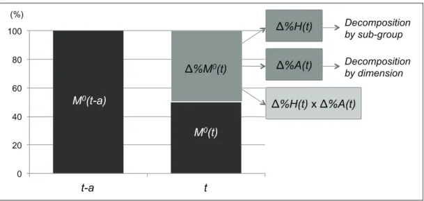
Figure 1.

Summary of decomposition of changes

0 20 40 60 80 100

t-a t

M

_(t-a)

M

_(t)

%M

_(t)

%H(t)

%A(t)

%H(t)

x

%A(t)

In a nutshell, the method decomposes changes in the adjusted headcount ratio ( _M0) between two periods (t−a and t) into changes in the headcount ratio (Δ%H(t)) and the average deprivation of poor people (Δ%A(t)), as demonstrated in Figure 1. Subsequently,

Δ%H(t) can be further decomposed into sub-group changes; while Δ%A(t) can be further decomposed into changes in headcount poverty by dimension/variable (as shown below). Additionally, with panel data, Δ%H(t) can be linked to the probabilities of entry into and exit from multidimensional poverty; while (Δ%A(t)) can be linked to the probabilities of entry into and exit from multidimensional poverty and being deprived in a specific dimension. Some additional alternative decompositions of Δ%_M0

(_t) are also provided.

2.1

General results for cross-sectional and panel data

The following results apply to any dataset, but the cross-sectional notation is used for simplicity. Denoting Δ%Y(t)=Y(t)−Y(t−α)

Y(t−α) and simplifying notation a bit, the first

straightforward result is the following:

Δ%M(t)=Δ%H(t)+Δ%A(t)+Δ%H(t)×Δ%A(t) (6) In other words, a percentage change in M0

can be decomposed into the percentage change in the number of multidimensionally poor people, the percentage change in the average number of deprivations of the multidimensionally poor, and a multiplicative effect. Figure 2 illustrates this decomposition.

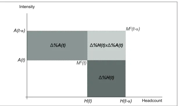
Figure 2.

Decomposition of changes in the adjusted headcount ratio M

The initial normalised multidimensional poverty level is represented by the rectangle

M 0

(t=0)

that could be understood as the product of A(t=0) and H(t=0). Any area smaller area than the one represented by ΔM0(t=0) implies a reduction in the multidimensional poverty level. In this specific case, the final level of multidimensional poverty

M 0

(t=1) is the result of the reduction in the headcount ratio Δ%H and in the average deprivation Δ%A. We eliminate the double counting of these changes by including a multiplicative factor Δ%A×Δ%H.

M

_{(t- )}

H(t- )

A(t- )

H(t)

A(t)

%A(t)

%H(t)

%H(t)

x

%A(t)

M

_(t)

Note that Δ%H(t) and Δ%A(t) are not independent, but there are circumstances in which a change in one may not necessarily produce a change in the other; for instance, in the extreme case of identifying poor people by the intersection approach, i.e. with k=D:Δ%A(t)=0 and so Δ%M0

(t)=Δ%H(t). Another circumstance in which a change in one element may not necessarily produce a change in the other element is when the proportion of

multidimensionally poor people remains the same, but the number of their deprivations increases. For this to happen it is necessary that k<D.

The result in equation (6) can be further expanded by decomposing both Δ%H(t) and

Δ%A(t). In the case of changes in H it may be interesting to decompose it in terms of changes in the multidimensional headcount for different groups of society. We do this by partitioning society in G non-overlapping groups, recalling that:

H(_t)= Ni t NtH i₍ t) i=1 G

∑

∑

t _{is the number of individuals belonging to group}

i in period t. From equation (8) it is clear that: Δ%H(t) = Δ% Nl t NtH i (t) ⎡ ⎣ ⎢ ⎤ ⎦ ⎥ri i=1 G

∑

∑

The result of equation (10) indicates that the percentage change in the multidimensional headcount can be decomposed into changes in the composition of the population

(Δ%_Nit_/

Nt), changes in the percentage of multidimensionally poor people within each group

(Δ%_Hi₍

t)), and a multiplicative effect. The relative impact of such changes depends on the initial contributions of every group headcount to the total, i.e. they depend on ri=

Ni t

Nt

Hi(_t−a)

H(_t−a)

which is the number of poor people in group i over the total poor people. Similarly Δ%A(t) can also be decomposed since A(t)=

d=1

D

∑

D Ad(t) and Ad(t) is the

percentage of multidimensionally poor people deprived in dimension d. Using a similar decomposition as in equations (8) and (10), the following decomposition is also derived:

Δ%A(t)= Δ% d=1 D

∑

∑

A(_t−a) . Note that Δ%A(t) is only affected by Δ%Ad(t), by mediation of the

sd, because we keep the dimensional weights constant. Otherwise equation (11) would look

2.2

Specific results for panel data

In the case of panel datasets _Nt

=N∀t, the same individuals are tracked across the different time periods. Therefore, for instance, Δ%H(t) can be decomposed into the transition

probabilities of moving into and out of multidimensional poverty:

Δ%H t

( )

(

)

(

₍

(

₎

)

)

(

)

<k) is the (transition) probability of being poor in period t conditional on having been non-poor in period t−a, i.e.

Pr(cn t_≥ k|cn t_a_< k)= 1 N[1−H(t−a)]_n=1I N

∑

k) is the (transition) probability of leaving multidimensional poverty

n in period t for people who were poor in period t−a, i.e.

Pr(cn t <k|cn t−a ≥k)= 1 NH(t−a) I(cn t <k∧cn t−a ≥k) n=1 N

∑

H(_t−a) is the ratio of non-poor to

poor people in the population in period t−a.

Note that equation (12) can also be expressed in terms of the persistence probabilities,

Pr(cn t _< k|cn t−a_< k)=1−Pr(cn t _≥ k|cn t−a_< k) and Pr(cn t _≥ k|cn t−a_≥ k)=1−Pr(cn t _< k|cn t−a_≥ k). Similar decompositions can be performed for the multidimensional headcounts of sub-groups within the population.

Δ%A(t) can also be further decomposed when panel data are available, by decomposing

Δ%Ad(X t

;Z) in terms of different kinds of poverty transition probabilities. For instance, note that: Ad(t)= Pr(_xndt <zd∧cn t ≥k) H(_t) (13) where Pr(_xndt <zd∧cn t

≥k) is the probability of being multidimensionally poor and deprived in variable d. It is a poverty headcount of d censored by multidimensional poverty status. In order to ease notation, we define

CHd(t)=Pr(xnd t

<zd∧cn t

≥k). From equation (13) it is clear that:

Δ%Ad(t)=

1+Δ%CHd(t)

1+Δ%H(t) (14)

The denominator of equation (14) depends on Δ%H(t), which was decomposed in terms of transition probabilities in equation (12). The numerator features Δ%_CHd(_t), i.e. the

percentage change in the censored headcount of d. An expression of it in terms of transition probabilities is analogous to that in equation (12):

Δ%_CHd(_t)=Pr(_xndt _< zd∧cn t _≥ k|_xndt−a_> zd∨cn t−a_< k)1+CHd(t−a) 1+CH(t−a) +Pr(xnd t _≥ zd∨cn t _< k|xnd t−a_≤ zd∧cn t−a_≥ k) (15)

Now the censored headcount depends on two conditions, i.e. being multidimensionally poor and being deprived in a specific dimension. Hence the transition probabilities into and out of the specific poverty status defined by the censored headcount depend on changes in both conditions.

To summarise, the change in the proportion of poor people deprived in variable

d,Ad,

depends on a complex interplay between the transition probabilities into and out of multidimensional poverty and the transition probabilities into and out of multidimensional poverty coupled with deprivation in variable d. The analysis of changes in

Ad can be done at

different levels of detail in the decomposition. It may focus on equation (14), or on the combination of equation (13) with equations (14) and (15).

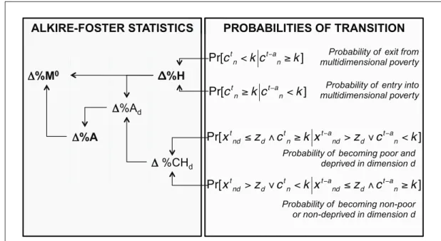
Thus far, the decompositions outlined in equation (6) and equations (11) to (15), are related to one another. Figure 3 expresses the logical links between them, emphasising the pathways through which the transition probabilities ultimately impact on M0.

Figure 3.

Decomposition of Alkire-Foster statistics based on transition

2.3

Alternative decompositions and a dominance result

There is, first, an alternative novel procedure that decomposes Δ%M0(t) in terms of Δ%H(t), without the appearance of Δ%A(t). The starting point is an equation describing M0

(t,k) as a linear combination of several multidimensional headcounts, derived by Alkire and Foster (2010). Now M0

(t,k) denotes the adjusted headcount ratio as a function of the multidimensional cut-off: M0(_t,_k)= 1 D kH(t,k)+_j=k+1H(t,j) D

∑

(t,k) is equal to a weighted sum of all the headcounts from a multidimensional cut-off of k up until D. Computing the percentage change on both sides of equation (16), and rearranging, yields:

Δ%M0(t,k)= kH(t−a,k) DM0(t−a,k)Δ%H(t,k)+ H(t−a,j) DM0(t−a,j) j=k+1 D

∑

PROBABILITIES OF TRANSITION

ALKIRE-FOSTER STATISTICS

%A

%H

%A

%CH

%M

Pr[

c

<

k c

k

]

Pr[

c

k c

<

k

]

Pr[

x

z

c

k x

>

z

c

<

k

]

Pr[

x

>

z

c

<

k x

z

c

k

]

Probability of exit from multidimensional poverty

Probability of becoming poor and deprived in dimensiond

Probability of becoming non-poor or non-deprived in dimension d

According to equation (17),Δ%M0

(t,k) can be expressed as a weighted average of all the

Δ%H(t,j) from j=k until D. The weights depend on the initial values of the respective H and M0. With equation (17) we also derive the following dominance condition:

Δ%H(t,k)]b≤[Δ%H(t,k)c∀k=[1,D]→ Δ%M0(t,k)b≤ Δ%M0(t,k)c∀k=[1,D] (18) Where b and c represent two different countries or regions; e.g. [Δ%H(t,k)]b _{stands for the}

change in the headcount in region b. Condition (18) states that if region b experiences a higher reduction (or lower increase) in the multidimensional headcount than country c for all values of k, then it will also exhibit a higher reduction (or lower increase) in the adjusted headcount ratio for all values of k. Linking this result to equation (12) yields the following condition: Pr(ci t_≥ k|ci t−a_< k)b≤Pr(ci t_≥ k|ci t−a_< k)c∧ Pr(ci t_< k|ci t−a_≥ k)b≥Pr(ci t_< k|ci t−a_≥ k)c ∀k=[1,D]→ Δ%H(t,k)b_{≤ Δ%H(t,k)}c _{∀k=[1,D]→} Δ%M0(t,k)b≤ Δ%M0(t,k)c ∀k=[1,D]→ (19)

Condition (19) states that if, for all values of k, the entry probabilities in b are not higher than in c and the exit probabilities in b are at least as high as c’s, then b experiences higher reduction (or lower increase) than c in H, and then in M0

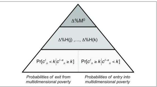
, for all values of k. This condition is related to the more direct link between the transition probabilities and Δ%M0

(t,k) that ensues when equation (12) is combined with (17). Figure 4 illustrates this connection.

Figure 4.

Changes in the adjusted multidimensional headcount based on transition

probabilities

There is another procedure that decomposes, Δ%M0

(t,k) but this time only in terms of changes in each of the censored headcounts, i.e.Δ%CHd(t,k) (which in turn can be

decomposed into their respective transition probabilities, as in equation (15)). To attain this result first note that plugging equation (14) into equation (11) yields:

%M

Pr[

c

<

k c

k

]

%H(

j

) ,…, %H(k)

Pr[

c

k c

<

k

]

Probabilities of exit from multidimensional poverty

Probabilities of entry into multidimensional poverty

Δ%A(t,k)= 1+ sdΔ%CHd(t,k) d=1 D

∑

Then plugging equation (20) into equation (6) yields the decomposition of Δ%M0

(t,k) in terms ofΔ%CHd(t,k): Δ%M0 (t,k)= sdΔ%CHd(t,k) d=1 D

∑

Equation (21) states that Δ%M0

(t,k) is a weighted sum of the percentage changes in each of the censored headcounts, where the weights are given by sd =

wd

D

CHd(t−a,k)

M0(t−a,j) ; i.e. the

contribution of the censored headcount to the adjusted headcount ratio in the initial period. The relationship linking the transition probabilities into and out of the censored headcounts to the adjusted headcount ratio is illustrated in Figure 5.

Figure 5.

Changes in the adjusted multidimensional headcount based on transition

probabilities using dominance properties

Pr[

x

z

c

k x

>

z

c

<

k

]

Pr[

x

>

z

c

<

k x

z

c

k

]

dimension d Probability of becoming non-poor or non-deprived in dimension d

%M

%CH(1) ,…, %CH(D)

3.

Data

We use the panel dataset collected by Young Lives, an international study of childhood poverty carried out in Andhra Pradesh (India), Ethiopia, Peru and Vietnam. The first three rounds of the survey collected information on children’s individual, household and communal characteristics in 2002, 2006–7 and 2009. We focus the analysis on the Older Cohort, who were 8 years old in 2002. The final sample includes only those individuals in all three survey rounds without missing values for the selected indicators. Table 1 shows basic information on the four samples. Interestingly the rural composition of the sample exhibits significant

changes, with the exception of Ethiopia.

Table 1.

Sample

characteristics

Survey round Original sample Selected sample Mean age Females (%) Rural (%)

Ethiopia 1 1,000 868 7.88 49.1 61.2 2 980 868 12.05 60.7 3 973 868 14.56 59.7 Andhra Pradesh 1 1,008 944 7.98 50.6 75.6 2 994 944 12.32 74.8 3 975 944 14.72 57.1 Peru 1 714 660 7.93 47.0 26.1 2 685 660 12.31 40.3 3 678 660 14.44 23.6 Vietnam 1 1,000 957 7.97 50.4 80.6 2 990 957 12.25 69.3 3 974 957 14.73 n.a.

Table 2 shows the variables that we have chosen considering both the vast literature on multidimensional child poverty and the availability of data. We opted to combine variables that measure functionings, or capabilities, exclusively attributable to the individual, and variables that measure household environment and are not exclusively attributable to the child (e.g. his/her siblings would receive the same value). The individual variables measure three human-capital functionings, which in turn affect future human capital: child work, school attendance and nutrition. Seven of the eight chosen variables measuring household

environment provide information on the children’s capability to live in a household with adequate electricity, cooking fuel, drinking water, toilet, space (i.e. no overcrowding), access to basic household assets (e.g. radio, fridge, phone, etc.). The other variable is a measure of child mortality in the household, proxying low outcomes in the household production function of health and well-being. All indicators have the same weight (1/11)

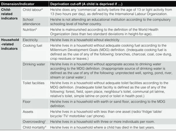
Table 2.

Child poverty dimensions

Dimension/Indicator Deprivation cut-off (A child is deprived if …)

Child-related indicators

Child laboura _{He/she does any ‘commercial’ activity before the age of 13 or light activity from}

13 (two hours per day), as defined by the International Labour Organization. School

attendance

He/she is not attending an educational institution according to the compulsory schooling level of his/her country.

Nutritionb _{He/she is malnourished according to the definition of the World Health}

Organization (less than two standard deviations in height-for-age).

Household -related indicators

Electricity He/she lives in a household wihout electricity

Cooking fuel He/she lives in a household without adequate cooking fuel according to the Millennium Development Goals (MDG) definition. (Indequate cooking fuel is defined as the use of any of the following: branches, charcoal, coal, cow dung, crop residues or leaves.)

Drinking water He/she lives in a household without appropiate access to drinking water according to the MDG definition. (Inappropriate source of drinking water is defined as the use of any of the following: unprotected well, spring, pond, river, stream or canal water.)

Toilet facilities He/she lives in a household without adequate toilet facilities according to the MDG definition. (Inadequate toilet facility is defined as the use of any of the following: forest, field, open place, neighbour’s toilet, communal pit latrine, relative’s toilet, simple latrine on pond or toilet in health post.)

Floor He/she lives in a household with earth or sand floor, according to the MDG definition.

Assets He/she lives in a household with less than one asset (radio/ fridge/ table/ bicycle/ TV/ motorbike/ car/ phone).

Overcrowdingc _{He/she lives in a household with three or more individuals per room.}

Child mortalityd _{He/she lives in a household where a child has died in the last years.}

a ILO Convention 138, http://www.ilo.org/ilolex/cgi-lex/convde.pl?C138 b Child growth standards, http://www.who.int/childgrowth/software/en

c The MDGs use this overcrowding indicator to identify a slum; however, it is not included directly as a goal: http://www.childinfo.org/mdg.html

d Round 1 includes all periods (before). Rounds 2 and 3 only cover the change periods between interviews.

The literature offers many other options, which stem from different ways of understanding the nature of child poverty, and also require additional information. Some authors draw their lists from development goals agreed upon in different meetings. For instance, Gordon et al. (2005) base their choices on the World Summit on Social Development, while the choices by Roche (2010) are informed by the Millennium Development Goals and by the World Summit for Children. In this paper, we do not explicitly seek to justify our choices in terms of a specific worldwide agreement, but rather on the grounds of measuring aspects of the children’s functionings and capabilities, parsimony, comparability across the four datasets, and data availability.

An important distinction in the literature is the one between ‘conventional’ and subjective measures of non-income child poverty (White et al. 2003). While some of our variables are close to the conventional indicators mentioned by White et al., we do not use others like teenage pregnancy because we want to have as much commonality in the variables across genders as possible. We have also decided not to add purely subjective measures to the set for the sake of clarity and comparability across the different cultures embedded in the countries and regions of the Young Lives study. More recent approaches to choices of dimensions and indicators have taken different routes.

substantial range of indicators describing dwelling conditions. Child work and school

attendance have rightly received universal consideration in the recent literature (including the measurement of child well-being, see Fernandes et al. 2012). By contrast, children’s health has not always been considered, and when it has been considered, the range of indicators has been wide. For instance, Biggeri et al. (2010) consider access to drinking water as a measure of health, whereas Roche (2010) looks at measles immunisation and Roelen (2010) measures health poverty by considering visits to health facilities run by professionals.

Clearly, data availability explains, at least partly, such different choices. In this respect, we decided to include one indicator of child nutrition (height-for-age) and to include some dwelling environment conditions that affect a child’s health.

Several other environmental variables have been considered in the literature, but without the cross-study consistency observed for variables like school enrolment and child work. For instance, Notten and Roelen (2010) use several measures of financial means to afford different assets and they also consider several indicators of neighbourhood quality and access to public services. By contrast, Roelen (2010) accounts for whether the caregiver is disabled; Biggeri et al. (2010) have added measures of children’s autonomy; Bastos and Machado (2009) have a whole module of indicators on children’s social integration; and Gordon et al. (2005) consider measures of information deprivation.

Panel studies on child poverty have to deal with changes in the type and structure of relevant dimensions as the individual grows up. The welfare determinants of a child under 5 are mostly related to his/her health and parental care. However, after this point other dimensions might become more relevant, such as child work or education. In this regard, there is a trade-off between the selection of comparable indicators across time, and the ability to capture the crucial conditions of a child at each point of his/her life.

In this paper, we have focused the analysis on indicators that relate to the individual child and to his/her closest environment, i.e. the dwelling and the household. Unlike other studies, we have not chosen explicitly several indicators for each dimension, in order to keep the number of variables manageable. For instance, some studies, like ours, use one indicator of education (e.g. Biggeri et al. 2010), whereas others use several (Roelen 2010). But the latter is partly due to the fact that studies that use several indicators of one dimension usually measure poverty at the household level, therefore considering children from different age brackets for whom different aspects of the same dimension may be relevant (e.g. school enrolment versus completion, as in the case of Roelen (2010). By contrast, we focus on just one cohort of children.

The selection of dimensions/variables in this paper seeks to balance the methodological requirements for increasing the comparability with the need to collect information about how an individual’s well-being evolves. To address this issue several strategies have been

implemented. First, the literature suggests that dimensions are more stable over time after the age of 5, and this paper includes individuals from the Young Lives Older Cohort only. Secondly, only standard indicators are presented in this final version, based on consensus around the relevant indicators for children aged between 8 and 14. Third, the selection of the child-related dimensions was based on more temporal robust indicators like height-for-age (instead of BMI, as in the first version of this paper). Also, the child work indicator recognises the different conditions at different ages by adapting the deprivation cut-off to the specific age of the child.1

Finally, as was mentioned before, dimensions have been classified into two sub-groups: one related to the child, and the other related to the household, in order to address in detail the context in which the deprivation arises. This classification could help to explain the relevance of external variables related to the household and consequently not to the age of the

individual and, at the same time, variables that are age-specific. It is not within the scope of this paper to provide a detailed analysis of the child at different ages, but to analyse changes over time using a set of pre-defined dimensions.

4.

General results

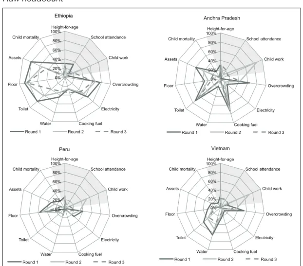
Figure 6 shows the raw deprivations by country and survey round. These raw deprivations are the percentages of children who are poor in one specific variable, regardless of whether they are deemed multidimensionally poor. In other words, these are headcounts uncensored by multidimensional poverty status (i.e different from CHd(t)). For instance, the raw

deprivation headcount of dimension d is:

H_d(t)= 1

Nt _n=1I(xnd ≤zd)

Nt

∑

Figure 6.

Raw

headcount

0% 20% 40% 60% 80% 100% Height-for-age

School attendance Child work Overcrowding Electricity Cooking fuel Water Toilet Floor Assets Child mortality

Andhra Pradesh

Round 1 Round 2 Round 3 0% 20% 40% 60% 80% 100% Height-for-age

School attendance Child work Overcrowding Electricity Cooking fuel Water Toilet Floor Assets Child mortality Ethiopia Round 1 Round 2 Round 3 0% 20% 40% 60% 80% 100% Height-for-age

School attendance Child work Overcrowding Electricity Cooking fuel Water Toilet Floor Assets Child mortality Peru Round 1 Round 2 Round 3 0% 20% 40% 60% 80% 100% Height-for-age

School attendance Child work Overcrowding Electricity Cooking fuel Water Toilet Floor Assets Child mortality Vietnam Round 1 Round 2 Round 3

The results in this section are a good starting point to document the nature of

multidimensional child poverty in the four countries studied. However, note that they do not say much about the extent of joint multiple deprivations. For all the countries, significant reductions in the raw headcounts took place between Round 1 and Round 3, although not always monotonically; and there are a few exceptions (e.g. deprivation in cooking fuel in Ethiopia). Also the figure reveals different patterns of raw deprivation across the countries. For instance, in Andhra Pradesh overcrowding, lack of adequate sanitation and cooking fuel deprivation remain important. By contrast, floor quality stands out in Peru, while access to drinking water is more relevant in Vietnam. Of course, there are also similarities. For instance, overcrowding is highly relevant in the four countries, and floor quality is the most relevant dimension, in terms of deprivation, both in Ethiopia and Peru.

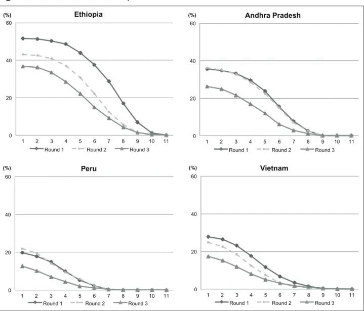
Figure 7.

Evolution of the adjusted headcount ratio M

Figure 7 shows the estimates of the adjusted headcount ratio, _M0, for the four countries, three survey rounds and all multidimensional cut-offs based on natural numbers. All countries show progress in terms of poverty reduction from Round 1 to Round 3, yet the patterns differ. For instance, the poverty profiles in Peru and Andhra Pradesh are very similar in Rounds 1 and 2. But then clear progress occurs from Round 2 to Round 3. Comparing across

0 20 40 60 1 2 3 4 5 6 7 8 9 10 11 (%) Ethiopia Round 1 Round 2 Round 3 0 20 40 60 1 2 3 4 5 6 7 8 9 10 11 (%) _{Andhra Pradesh} Round 1 Round 2 Round 3 0 20 40 60 1 2 3 4 5 6 7 8 9 10 11 (%) _Peru Round 1 Round 2 Round 3 0 20 40 60 1 2 3 4 5 6 7 8 9 10 11 (%) _Vietnam Round 1 Round 2 Round 3

countries, the Peruvian sample stands out as the least poor, followed by those of Vietnam and Andhra Pradesh. Then the Ethiopian sample is the poorest of the four. This pattern remains robust across survey rounds and multidimensional poverty cut-offs.

Table 3, and Figures 12 and 13 (in the Appendix) also document levels, but now those of H

and A. The trends for H are similar to those for _M0: progress from Round 1 to Round 3 but not always monotonic (for example, Peru faced some increases in H at low levels of k from Round 1 to Round 2). The cross-country patterning is also the same: Peru is the least poor in terms of H, followed by Vietnam, Andhra Pradesh and Ethiopia. By contrast, both the trends and the relative rankings related to A are much less consistent. In terms of trends, the four countries exhibit increases in the average number of deprivations at least for one value of k. As for rankings, in several cases, the values of A in a pairwise comparison are too close to venture any meaningful statement. The patterning found for A is much less clear than those for _M0 and H.

5.

Dynamic results

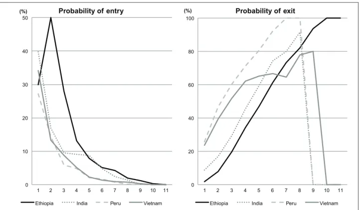
Table 4 (in the Appendix) and Figure 8 show the transition probabilities into and out of multidimensional poverty for the four countries’ samples and all posible poverty cut-offs (natural values of k). The two intermediate transitions are reported in Table 4 and the total transitions from Round 1 to Round 3 are illustrated in Figure 8.

Figure 8.

Probabilities of entry into and exit from multidimensional poverty by cut-off:

Rounds 1 to 3

Ethiopia India Peru Vietnam

0 20 40 60 80 100 1 2 3 4 5 6 7 8 9 10 11 (%) _{Probability of exit}

Considering that the conditions for multidimensional poverty identification become more demanding as we move from a union to an intersection approach, i.e. from low to high values of k, it is not surprising that the exit probabilities tend to be higher as k increases. Likewise, it is reasonable to observe, as we do, higher entry probabilities for lower values of k. Note though that these trends are not entirely mechanical, or trivial. For instance, between Rounds 2 and 3 the exit probabilities in Ethiopia are higher when k=9 than when k=10. Likewise, for Vietnam in the same period, the exit probability for k=4 is very similar to that for k=5. The cross-country comparisons reveal that no country clearly shows higher exit probabilities than all the others between Rounds 1 and 2. However, people in Peru and Vietnam were more able to transition out of poverty than those in Ethiopia and Andhra Pradesh. Within each of these two pairs no country dominates though. Between Rounds 2 and 3, the ranking situation changes: Peru exhibits the highest exit rates for all k, while Ethiopia exhibits the lowest. Between Vietnam and Andhra Pradesh the comparison depends on the choice of k. All countries, except Vietnam, exhibit consistently higher exit probabilities during Round 2. As for the probability of becoming multidimensionally poor, again, no country stands out for every k and between Rounds 1 and 2, although people in Peru were less likely to fall into multidimensional poverty than those in Ethiopia and Andhra Pradesh. Interestingly, the exit probabilities between Rounds 1 and 2 for all countries fall sharply when k goes from 1 to 2, with the exception of Ethiopia. For all countries there is a significant drop in entry probabilities between Rounds 2 and 3, although this is not always true in some countries for k values close to the intersection approach, which involve relatively smaller groups of people. Between Rounds 2 and 3 Peru again stands out as the most well-off country, in this case with the lowest entry rates. People in Andhra Pradesh were less likely to become poor than people in Ethiopia, but there were no clear differences in this probability between Vietnam and Andhra Pradesh, or Vietnam and Ethiopia.

Figure 8 shows the entry and exit probabilities between Round 1 and Round 3. Like the results in Table 4, entry probabilities tend to decrease with higher values of k, while exit probabilities undergo an opposite trend. However, these tendencies are not purely monotonic, as exemplified by the probabilities of becoming multidimensionally poor in Ethiopia or the probabilities of transitioning out of poverty in Vietnam. This is a hint that the behaviour of the transition probabilities along different values of k is not simply mechanical. Entry probabilities appear very high for low levels of k, with Ethiopia showing the highest ones, followed by Andhra Pradesh. Those of Peru and Vietnam are lower and very similar to each other. As for exit probabilities, the years between Rounds 1 and 3 have seen complete transitions (100 per cent) out of multidimensional poverty for high levels of k and for all countries. In the case of Peru, this is the case from k=6 upward. All the others experience complete transitions from k=9 upward. In other words, all countries have witnessed

multidimensional child poverty disappear for the identification criteria that are closest to the pure intersection approach. Peru exhibited the highest exit probabilities. Rates in Andhra Pradesh were higher than those in Ethiopia. The other pairwise comparisons are

inconclusive.

Figure 14 (in the Appendix) shows the entry and exit probabilities between Round 1 and Round 2, and between Round 2 and Round 3. Interestingly the entry probabilities tend to be lower between Rounds 2 and 3, for the four samples and for low values of k. By contrast, for relatively high values of k there is not much difference between the transition probabilities between the survey rounds, although these probabilities are low to begin with. In the four countries the most significant reduction in entry probabilities occurs with identification

approaches at, or very close to, the union approach, i.e. the mildest forms of

multidimensional deprivation. Progress in the form of increases in exit probabilities, between Rounds 1 and 2, and 2 and 3, is not as widespread across the four samples as progress in the form of reductions in entry probabilities. On the one hand, Andhra Pradesh and Peru exhibit significant increases in exit probabilities between Rounds 2 and 3, for most values of

k. On the other hand, for several values of k, exit probabilities are actually lower between Rounds 2 and 3 than between Rounds 1 and 2, in Ethiopia and Vietnam.

6.

Decomposition results

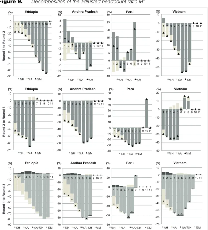
Figure 9, and Table 5 in the Appendix, show the decomposition results based on equation (6) for different values of k. For most countries and most values of k, the main driver of changes in _M0 is the change in H. The few exceptions appear with low values of k, i.e. identification criteria at, or close to, the union approach.

Figure 9.

Decomposition of the adjusted headcount ratio M

Figure 10 and Table 6 (in the Appendix) shows the decomposition results based on equation (10). The exit probabilities are compared against an ‘adjusted’ entry probability. The latter is simply the first element of the right-hand side of (10), i.e. Pr(cn

t ≥kcn

t−a

<k)1−H(t−a)

H(t−a) . Note

that this element also increases with k. The reason is that, even though entry probabilities do decrease as we move towards intersection approaches, the ratio 1−H

H also increases when

going in the same direction. Moreover, this increase seems to be greater than the decrease in the entry probabilities.

-90 -80 -70 -60 -50 -40 -30 -20 -10 0 10 1 2 3 4 5 6 7 8 9 10 11 (%) Ethiopia %H %A %M -12 -10 -8 -6 -4 -2 0 2 4 6 8 10 1 2 3 4 5 6 7 8 9 10 11 (%) Andhra Pradesh %H %A %M -10 -5 0 5 10 15 20 25 30 1 2 3 4 5 6 7 8 9 10 11 (%) Peru %H %A %M -60 -50 -40 -30 -20 -10 0 10 1 2 3 4 5 6 7 8 9 10 11 (%) Vietnam %H %A %M -40 -30 -20 -10 0 10 20 30 40 50 60 1 2 3 4 5 6 7 8 9 10 11 (%) Peru %H %A %M -70 -60 -50 -40 -30 -20 -10 0 10 1 2 3 4 5 6 7 8 9 10 11 (%) Andhra Pradesh %H %A %M -70 -60 -50 -40 -30 -20 -10 0 10 1 2 3 4 5 6 7 8 9 10 11 (%) Ethiopia %H %A %M -50 -40 -30 -20 -10 0 10 20 1 2 3 4 5 6 7 8 9 10 11 (%) Vietnam %H %A %M -90 -80 -70 -60 -50 -40 -30 -20 -10 0 10 1 2 3 4 5 6 7 8 9 10 11 (%) Ethiopia %H %A %A*%H %M -70 -60 -50 -40 -30 -20 -10 0 10 1 2 3 4 5 6 7 8 9 10 11 (%) Andhra Pradesh %H %A %A*%H %M -80 -60 -40 -20 0 20 40 1 2 3 4 5 6 7 8 9 10 11 (%) Peru %H %A %A*%H %M -70 -60 -50 -40 -30 -20 -10 0 10 1 2 3 4 5 6 7 8 9 10 11 (%) Vietnam %H %A %A*%H %M R ound 1 to R ound 2 R ound 2 to R ound 3 R ound 1 to R ound 3

Figure 10.

Decomposition of changes in the H

Hence, this ‘adjusted’ entry probability also increases with k. As Figure 10 and Table 6 (in the Appendix) show, there were greater reductions in H in Ethiopia and Vietnam than in Peru and Andhra Pradesh between Rounds 1 and 2. By contrast, between Rounds 2 and 3, the greatest reduction in H was in Andhra Pradesh, while the reductions in H in most other countries depend on the value of k. In particular, Ethiopia, Peru and Vietnam exhibit some sharp percentage increases in H for high values of k. These though involve relatively small numbers of children at the baseline (hence the high percentage increases). Another

-150 -100 -50 0 50 100 150 1 2 3 4 5 6 7 8 9 10 11 (%) Ethiopia Probability of exit Adjusted probability of entry % H -100 -50 0 50 100 150 1 2 3 4 5 6 7 8 9 10 11 (%) Andhra Pradesh Probability of exit Adjusted probability of entry % H -100 -50 0 50 100 150 1 2 3 4 5 6 7 8 9 10 11 (%) Peru Probability of exit Adjusted probability of entry % H -100 -50 0 50 100 150 1 2 3 4 5 6 7 8 9 10 11 (%) Vietnam Probability of exit Adjusted probability of entry % H -100 -50 0 50 100 150 1 2 3 4 5 6 7 8 9 10 11 (%) Ethiopia Probability of exit Adjusted probability of entry % H -100 -50 0 50 100 150 1 2 3 4 5 6 7 8 9 10 11 (%) Andhra Pradesh Probability of exit Adjusted probability of entry % H -100 -50 0 50 100 150 1 2 3 4 5 6 7 8 9 10 11 (%) Peru Probability of exit Adjusted probability of entry % H -100 -50 0 50 100 150 1 2 3 4 5 6 7 8 9 10 11 (%) Vietnam Probability of exit Adjusted probability of entry % H -100 -50 0 50 100 150 1 2 3 4 5 6 7 8 9 10 11 (%) Ethiopia Probability of exit Adjusted probability of entry % H -100 -50 0 50 100 150 1 2 3 4 5 6 7 8 9 10 11 (%) Andhra Pradesh Probability of exit Adjusted probability of entry % H -100 -50 0 50 100 150 1 2 3 4 5 6 7 8 9 10 11 (%) Peru Probability of exit Adjusted probability of entry % H -100 -50 0 50 100 150 1 2 3 4 5 6 7 8 9 10 11 (%) Vietnam Probability of exit Adjusted probability of entry % H R ound 1 to R ound 2 R ound 2 to R ound 3 R ound 1 to R ound 3

Going back to Figure 9, reduction of A was greater (or increases lower) in Ethiopia and Vietnam than in Peru and Andhra Pradesh between Rounds 1 and 2, for all values of k. Between Rounds 2 and 3, no pair-wise comparison is robust to the value of k. Also, within countries, whether A increased or decreased depends on the choice of second-stage identification threshold. As for the adjusted headcount ratio, Table 5, in the Appendix, shows that between Rounds 1 and 2, Vietnam experienced the highest reduction, followed by Ethiopia. Andhra Pradesh and Peru experienced the lowest reductions, but their pair-wise comparison depends on the value of k. Between Rounds 2 and 3, the only result robust to changes in k is that Andhra Pradesh experienced higher reductions than Ethiopia. During the same period, some countries experienced increases in M0 for intersection approaches (involving few people at the baseline).

Figure 11.

Decomposition of changes in the A

-20 -15 -10 -5 0 5 10 15 1 2 3 4 5 6 7 8 9 10 11 (%) Ethiopia

Adjusted contribution HH dimensions Adjusted contribution childdimensions %A -20 -15 -10 -5 0 5 10 15 1 2 3 4 5 6 7 8 9 10 11 (%) Andhra Pradesh

Adjusted contribution HH dimensions Adjusted contribution childdimensions %A -20 -15 -10 -5 0 5 10 15 1 2 3 4 5 6 7 8 9 10 11 (%) Peru

Adjusted contribution HH dimensions Adjusted contribution childdimensions %A -20 -15 -10 -5 0 5 10 15 1 2 3 4 5 6 7 8 9 10 11 (%) Vietnam

Adjusted contribution HH dimensions Adjusted contribution childdimensions %A -40 -30 -20 -10 0 10 20 30 40 1 2 3 4 5 6 7 8 9 10 11 (%) Ethiopia -40 -30 -20 -10 0 10 20 30 40 1 2 3 4 5 6 7 8 9 10 11 (%) Andhra Pradesh

Adjusted contribution HH dimensions Adjusted contribution childdimensions %A

Adjusted contribution HH dimensions Adjusted contribution childdimensions %A -40 -30 -20 -10 0 10 20 30 40 1 2 3 4 5 6 7 8 9 10 11 (%) Peru

Adjusted contribution HH dimensions Adjusted contribution childdimensions %A -40 -30 -20 -10 0 10 20 30 40 1 2 3 4 5 6 7 8 9 10 11 (%) Vietnam

Adjusted contribution HH dimensions Adjusted contribution childdimensions %A -35 -25 -15 -5 5 15 25 1 2 3 4 5 6 7 8 9 10 11 (%) Ethiopia

Adjusted contribution HH dimensions Adjusted contribution childdimensions %A -35 -25 -15 -5 5 15 25 1 2 3 4 5 6 7 8 9 10 11 (%) Andhra Pradesh

Adjusted contribution HH dimensions Adjusted contribution childdimensions %A -35 -25 -15 -5 5 15 25 1 2 3 4 5 6 7 8 9 10 11 (%) Peru

Adjusted contribution HH dimensions Adjusted contribution childdimensions %A -35 -25 -15 -5 5 15 25 1 2 3 4 5 6 7 8 9 10 11 (%) Vietnam

Adjusted contribution HH dimensions Adjusted contribution childdimensions %A R ound 1 to R ound 2 R ound 2 to R ound 3 R ound 1 to R ound 3

Figure 11 and Table 7 (in the Appendix) show the most basic decomposition of A. For these results, the deprivations of the poor children have been grouped into deprivations exclusively attributable to the individual (e.g. child work) and those related to the individual’s household environment (e.g. electricity). this is achieved by adding up the respective Ad statistics

(equation 11) across the variables belonging to the same group. Figure 11 (in the Appendix) shows the relative contributions of the children-specific deprivations to total average

deprivation, A. Interestingly, for all countries and all values of k, these contributions increase (to the detriment of the contribution of household deprivations) from Round 1 to Round 3. For most (but not all) countries and values of k, this increase is also already patent when moving from Round 1 to Round 2. Then the results in Figure 11 show the decomposition of A

according to equation (9). The results do not reveal clear patterns. Rather the country experiences tend to be idiosyncratic and the trends depend on the choices of k. For instance, in Ethiopia and Vietnam, changes in household deprivations among the poor seem to be the key drivers of change in A for most values of k, but several exceptions appear. Strikingly, in most cases across countries, survey rounds and multidimensional cut-offs (k), changes in children-specific deprivations move in opposite directions to changes in household

deprivations. Vietnam’s pattern is interesting because, of the four countries, it is the only one in which the changes in A are positive between Rounds 2 and 3, for all values of k, between Rounds 2 and 3

7.

Multidimensional child poverty

assessments in the context of

the broader outlook of the Young

Lives economies

In this section we relate the trends in multidimensional poverty for the four Young Lives samples to economic conditions in their respective countries or region. While the Young Lives samples are not representative of their respective countries/region, we expect that their children may have been somewhat affected by surrounding economic phenomena at the macro level.

7.1 Andhra

Pradesh

As shown in the results above, Andhra Pradesh did not experience significant changes in multidimensional poverty between 2002 and 2006–7. However between 2006–7 and 2009 a substantial drop in poverty is apparent. Likewise during this second period, entry probabilities into poverty significantly decrease whereas exit probability significantly increase.

Interestingly these trends seem to coincide with a south-west monsoon below the average of 624 mm between 2001 and 2005. Thereafter the monsoon recovered up to 2009 and has been erratic since then. By contrast the north-east monsoon has been below average during most of the last decade, but generally it carries a bit more than a third of the rain brought by the south-west monsoon. Exports of agricultural products also seem to have behaved in

School drop-out rates also experienced a substantial decrease between 2006–7 and 2009, especially between Grades 1 and 7, but decreases also took place between Grades 8 and 10 (Government of Andhra Pradesh 2012: Annexe 8.5).

7.2 Ethiopia

As shown in the results above, multidimensional poverty in Ethiopia decreased substantially, albeit from a relatively high baseline, between 2002 and 2009, with a steeper decline

between Rounds 1 and 2 (between Rounds 2 and 3, exit probabilities did not improve significantly compared to the previous interval).

The decade has witnessed substantial GDP growth in Ethiopia, with many years exhibiting two-digit rates. This success, along with reductions in monetary poverty is attributed to government policies more conducive to private investment, public investments tackling bottlenecks (e.g., in energy), an export boom led by Chinese and Indian demand, and expansion of social services (Mwanakatwe and Barrow 2010). The results are also

observable in steady increases in school net enrolment rates, reductions in child malnutrition and under-5 mortality rates, as well as increases in electricity consumption, improved sanitation facilities and improved water sources in both rural and urban areas. In all cases, though, this welcome progress has emerged from a very low baseline. Hence Ethiopia continues being one of the poorest countries in the world by different standards and measures. Consistently, its Young Lives sample is the poorest of the four according to our multidimensional poverty measures.

7.3 Peru

As shown in the results above, multidimensional poverty in Peru, which was relatively low compared to the other three Young Lives countries/region, did not change much between Rounds 1 and 2 (2002 and 2006–7). However, a decrease in poverty took place between the last two survey rounds (2006–7 and 2009).

Straight after Round 1 of Young Lives in Peru, the country experienced an economic boom led mostly by commodity exports. However most of the benefits became apparent after 2005. For instance, both male and female unemployment rates increased between 2002 and 2005 and only thereafter experienced a steady decrease. Such trends can help explain decreases in child work. Meanwhile net primary enrolment rates remained steady over the 2002–9 period, whereas net secondary enrolment rates have significantly increased between 2004 and 2009 (World Bank 2012). Malnutrition prevalence, both in terms of height-for-age and weight-for-age also decreased between 2005 and 2008. The under-5 mortality rate has been decreasing steadily since 2002. Also, monetary poverty indicators, using national poverty lines, including urban and rural areas, show declines between 2002 and 2009, with steeper progress among urban areas between 2005 and 2009. However, using dollar-a-day lines poverty decline is still apparent but with a couple of years of minor poverty increases. By contrast, the multidimensional index shows a steady decline after 2006–7.

During the period of study, electricity consumption, urban sanitation and improved water sources in rural areas have steadly increased, and improved water sources have increased from 2007 onwards in urban areas. All these developments seem to be in tune with the patterns of multidimensional poverty observed in the Young Lives dataset for Peru.