2-27-2018
Working Paper Number 18003
Antebellum Labor Markets
Joshua L. RosenbloomIowa State University, [email protected]
Follow this and additional works at:https://lib.dr.iastate.edu/econ_workingpapers
Part of theEconomic History Commons,Growth and Development Commons,Income Distribution Commons,Industrial Organization Commons, and theInternational Economics Commons
Iowa State University does not discriminate on the basis of race, color, age, ethnicity, religion, national origin, pregnancy, sexual orientation, gender identity, genetic information, sex, marital status, disability, or status as a U.S. veteran. Inquiries regarding non-discrimination policies may be directed to Office of Equal Opportunity, 3350 Beardshear Hall, 515 Morrill Road, Ames, Iowa 50011, Tel. 515 294-7612, Hotline: 515-294-1222, email [email protected].
This Working Paper is brought to you for free and open access by the Iowa State University Digital Repository. For more information, please visit lib.dr.iastate.edu.
Recommended Citation
Rosenbloom, Joshua L., "Antebellum Labor Markets" (2018).Economics Working Papers: Department of Economics, Iowa State University. 18003.
Abstract
The United States economy was transformed in the period between American independence and the beginning of the Civil War by rapid population growth, the development of manufacturing, the onset of modern economic growth, increasing urbanization, the rapid spread of settlement into the trans-Appalachian west, and the rise of European immigration. These years were also characterized by an increasing sectional conflict between free and slave states that culminated in 1861 in Southern secession from the Union and a bloody and destructive Civil War. Labor markets were central to each of these developments, directing the reallocation of labor between sectors and regions, channeling a growing population into productive employment and shaping in important ways the growing North-South division within the country. Put differently, labor markets influenced the pace and character of economic development in the antebellum United States. On the one hand, the responsiveness of labor markets to economic shocks was an important factor in promoting economic growth; on the other, imperfections in labor market response to these shocks had significant effects on the character and development of the national economy.
Keywords
Labor Force, Wages, Slavery, Free Labor, Immigration, Industrialization Disciplines
Economic History | Growth and Development | Income Distribution | Industrial Organization | International Economics
By Joshua L. Rosenbloom Department of Economics
Iowa State University and NBER 27 February 2018
Abstract
The United States economy was transformed in the period between American independence and the beginning of the Civil War by rapid population growth, the development of manufacturing, the onset of modern economic growth, increasing urbanization, the rapid spread of settlement into the trans-Appalachian west, and the rise of European immigration. These years were also characterized by an increasing sectional conflict between free and slave states that culminated in 1861 in Southern secession from the Union and a bloody and destructive Civil War. Labor markets were central to each of these developments, directing the reallocation of labor between sectors and regions, channeling a growing population into productive employment and shaping in important ways the growing North-South division within the country. Put differently, labor markets influenced the pace and character of economic development in the antebellum United States. On the one hand, the responsiveness of labor markets to economic shocks was an important factor in promoting economic growth; on the other, imperfections in labor market response to these shocks had significant effects on the character and development of the national economy.
For economists, the labor market is a metaphor for the collection of institutions and organizations that connect the suppliers of labor services (workers) with the employers of those services. In contrast to organized exchanges, such as a stock exchange, the labor market is not localized in a particular place. Instead, information flows and transactions take place through a wide range of channels and rely on a complex set of formal and informal organizations and
institutions.1 Understanding how these institutions evolve over time, and what the consequence
of this evolution are for economic growth are the central questions for scholars interested in the history of labor markets.
Despite the distance between the economist’s metaphorical market and historical reality, the idealized market model provides a powerful organizing framework for thinking about how an economy’s labor is utilized. The next section of this essay summarizes the key features of this conceptual framework. The following sections examine, in turn the labor market institutions at the heart of the sectional rivalry between the North and South, the response of labor markets to industrialization, urbanization and westward expansion, and the market for agricultural labor. The essay concludes with a consideration of the performance of labor markets in the antebellum era as reflected in the available wage data.
The Labor Market Model
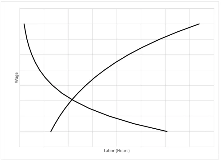
In the economist’s idealized world, a market is the place where buyers and sellers exchange a homogeneous good or service. In the labor market that good is labor services (L), measured in hours. The price of labor services is the wage rate (W). Employers’ demand for
labor services and workers’ supply of labor services interact in the market to determine a unique, equilibrium wage rate and quantity of labor services exchanged.
Figure 1 depicts this idealized market through plots of the aggregate demand and supply functions. The quantity of labor supplied is drawn as an increasing function of the wage rate. This positive relationship arises for two reasons: first, as wages rise, workers already supplying labor will be induced to provide more labor effort foregoing other activities as the value of their time at work increases; and, second, higher wages will cause some potential workers not working for wages to enter the market. The more responsive aggregate labor supply is to rising wages, the flatter the supply function will be. The demand for labor is drawn as a decreasing function of the wage rate. Employers demand for labor is derived from their ability to combine labor with other factors of production (capital, land, etc.) and natural resources to produce goods and services that can be sold at a profit. As the cost of labor rises, higher production costs will reduce the number of opportunities to profitably employ labor and will lead to reductions in employment. Employers may also be prompted to adopt new production techniques that replace labor with other factors of production as labor costs rise. Again, the slope of the demand function reflects employers’ responsiveness to wages. Economists measure the responsiveness of demand and supply in terms of “elasticity.” Elasticity is defined formally as the percentage change in quantity supplied or demanded that results from a one percent change in the wage rate.
The point at which supply and demand intersect, labeled as W*, L* is the unique
combination of wages and hours of labor at which the quantity of labor services employers wish to hire at the market wage rate equals the amount of labor services that workers wish to supply. At any other wage rate the quantity of labor supplied will not be equal to the quantity demanded and market participants will act in ways that cause wages to move toward W*. When the wage
Fig. 1. The Labor Market Model of Supply and Demand. The market wage rate and quantity of labor exchanged are determined by the point at which supply and demand curves intersect.
Wa
ge
is above W*, for example, the quantity of labor that workers wish to supply exceeds the quantity that employers want to employ. As a result, some workers will be unemployed or
underemployed. Seeing a labor surplus employers are likely to reduce wages and job seekers are likely to offer their services at a lower rate. Wages will continue to decline until they reach W*. On the other hand, if wages are below W*, the reverse will be true. In this case, employers desire more labor services than are being supplied, and there will be a shortage of labor.
Employers will compete with one another for the available workers, driving up wages until they reach W*.
The market equilibrium framework depicted in Figure 1 provides a way of analyzing the effects of a variety of labor market shocks. For example, an influx of immigrants to the labor market would increase the quantity of labor supplied at each wage rate. This would be depicted as a rightward shift of the entire labor supply function; the intersection of supply and demand would shift down and to the right along the demand function. This situation is illustrated in Figure 2. With the rightward shift in labor supply to Supply’, the equilibrium wage falls to W**, and the quantity of labor services employed increases to L**. A technological innovation that makes labor more productive would increase the quantity of labor employers demand at each wage rate and would be depicted as rightward shift of the demand curve. In this case, the new market equilibrium would occur to the right and above the old equilibrium.
An unstated assumption of the analysis so far is that the labor market illustrated in
Figures 1 and 2 has some geographic boundary. This might be a city or region, within which it is possible for workers to commute between their places residence and places of employment. An important issue historically, concerns the extent to which labor market conditions at one place are affected by those in other, geographically distinct locations. Differences in wages between
Fig. 2. Effects of a Positive Labor Supply Shock on Labor Market Equilibrium. A change in labor supply is reflected as a shift in the location of the labor supply curve. An increase in the supply of labor shifts the curve to the right, implying that at every wage a greater quantity of labor is supplied.] Wa ge Labor (Hours) Demand Demand
locations, if large enough, will induce the migration of workers toward places that offer higher earnings and/or the relocation of employment opportunities as employers seek lower cost sources of labor. In terms of the labor market model illustrated in Figures 1 and 2, migration of workers from low- to high-wage locations will increase labor supply at the high-wage location and reduce labor supply at the low-wage location. Other things equal, this will cause wages at the high-wage location to fall, and high-wages in the low-high-wage location to increase. Migration should continue until the difference in wages is too small to repay the costs of moving. A similar logic applies to employers’ location decisions. The smaller the differences in wages across locations and the more responsive workers and employers are to wage differentials across locations the greater the degree of geographic integration in the labor market. Declining costs of transportation and communication reduce the expenses to workers and employers of moving between distinct geographic locations and should be expected to result in movement toward an increasingly integrated national labor market.
The same logic used to analyze geographically separate labor markets can also be used to think about the relationship between markets for different occupations or skills. As with
migration workers and employers can shift between markets, but not without incurring costs. To make the analysis concrete, consider the markets for high school educated and college educated workers. Acquiring additional years of schooling is equivalent to the cost of migration from a low-wage to a high-wage location, and workers will invest in additional education if they expect this investment to be repaid. Similarly, employers can make investments in capital equipment or other aspects of the production process that allow them to substitute less educated workers for more educated ones in the same way that they can relocate from high- to low-wage locations.
Labor Market Institutions and Sectional Conflicts
Legal Foundations of Slavery and Free Labor
Perhaps the most distinctive feature of the labor market is that the labor services being exchanged are embodied in a human being. As the history of antebellum labor markets makes clear, legal definitions of property rights related to these services play a crucial role in shaping the transactions that can take place, and have important consequences that extend well beyond the labor market.
Before the American Revolution, a variety of different and overlapping arrangements concerning property rights in labor coexisted with one another in the territories that became the United States. At one end of the spectrum, the legal system sanctioned slavery, granting European Americans the right to own African Americans. Slave owners enjoyed relatively unrestricted control over the allocation of time and effort of their slaves as well as ownership of their offspring. Slaves could be freely bought and sold just as could any other form of property. At the other end of the spectrum, free colonists were able to enter into agreements to provide labor services for a limited period of time in transactions resembling those in contemporary labor markets. Between these two extremes were a number of intermediate arrangements, such as indentured servitude, in which free workers entered “voluntarily” into contracts to provide labor services, but once indentured they became the property of their master for the duration of the
contract, which was typically 3 to 4 years.2 During this period, masters could, freely exchange
indenture contracts without consulting with the servant.3
The Revolution marked an important turning point, however, in attitudes toward slavery,
at least in the Northern states, where slave numbers were limited.4 The Vermont state
from over sea, ought to be holden by law, to serve any person as a servant, slave or apprentice,
after he arrives at the age of twenty-one years, nor a female in like manner…”5 Other northern
states also adopted gradual emancipation in one form or another, ending with New Jersey, which did so in 1804. In southern states, where slaves made up 40 to 45 percent of the population, however, the defense of slavery only hardened.
At the Federal level, the emerging regional divergence was codified in the Northwest Ordinance. Drafted by Thomas Jefferson and passed by the Continental Congress in 1787, the Ordinance prohibited slavery in the territories north of the Ohio River and ensured that historical differences in the regional distribution of the use of slaves would be extended as population spread west. This division of the country between a free North and slave South was, as Gavin
Wright documents, in no sense an inevitable outcome.6 Many early settlers in Indiana and
Illinois advocated for making slavery legal, motivated by the opportunities to more rapidly develop productive farm land. But the provisions of the Northwest Ordinance prevented this, and the gradual build-up of free settlers in these territories shifted the balance of views.
The division of the country into two distinct regions characterized by different property rights regimes in the labor market contributed to the emergence of a uniquely American
conception of “free” labor. Efforts by slave owners in the north to circumvent abolition by claiming that slaves had entered freely into their relation of servitude led to a number of court cases. The logical culmination of which came in 1821, when the Indiana Supreme Court
concluded in the case of Mary Clark, a Woman of Color that employers could not impose
specific enforcement of a labor contract. While English courts at the time continued to hold that an indefinite labor contract was annual, and that a worker who left prior to the completion of this period was not entitled to compensation, American courts were increasingly inclined to rule that
workers who left an employer prior to the termination of their contract were entitled to compensation for the time they had worked. Thus, by the mid-nineteenth century the
employment relationship for free labor had been reconceptualized as a kind of lease agreement,
but one that could be maintained only so long as both parties assented to its continuation.7
Property Rights and Economic Development
The divergent patterns of economic growth in the North and South during the antebellum period, come as close to a natural experiment in the effects of institutional arrangements on economic development as history is likely to offer. In 1790, the two regions were nearly equal in population, land area and levels of wealth. Moreover, they shared a similar cultural heritage and were governed by the same national laws and institutions. By 1860, on the eve of the Civil War, the two regions had diverged along many dimensions. Compared to the North, the Southern population, was smaller, more rural and less densely settled. The region also had substantially lower levels of manufacturing employment, fewer miles of railroads per capita and had attracted
many fewer foreign immigrants.8
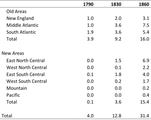
These differences in patterns of development are directly linked to the presence or absence of slavery. In both North and South, expansion onto the fertile soils of the trans-Appalachian West, facilitated by improvements in transportation and the growth of world markets for agricultural products, created enormous economic opportunities that were reflected in the rapid expansion of the settlement. This growth is charted in Table 1, which records population numbers at selected dates in the antebellum period. In 1790, virtually all of the nation’s population of 4 million lived east of the Appalachian Mountains, within the bounds of the original 13 states. Forty years later, in 1830, total population had more than tripled to nearly
13 million, of whom nearly 3 in ten lived in newly settled areas. By 1860, roughly half of a total population of 30 million lived outside the area of the original states.
Table 1: Regional Population (millions), selected dates, 1790-1860
1790 1830 1860 Old Areas New England 1.0 2.0 3.1 Middle Atlantic 1.0 3.6 7.5 South Atlantic 1.9 3.6 5.4 Total 3.9 9.2 16.0 New Areas
East North Central 0.0 1.5 6.9
West North Central 0.0 0.1 2.2
East South Central 0.1 1.8 4.0
West South Central 0.0 0.2 1.7
Mountain 0.0 0.0 0.2
Pacific 0.0 0.0 0.4
Total 0.1 3.6 15.4
Total 4.0 12.8 31.4
Source: Carter et al (2006, series Aa36-45)
Westward migration entailed significant costs and risks. Potential migrants had to gather information about the land they were considering buying, they had to finance the costs of
movement and the initial expenses of clearing land, building structures and planting crops before they could begin to reap the rewards of their move. In addition to these economic obstacles, there were also the psychic costs of leaving familiar places and relatives to move to the frontier.
These costs are in effect frictions that slowed the response to the potential rewards of migration. In the South, however, the presence of slavery and the market in human labor it implied substantially reduced the impact of these frictions. The existence of an active inter-regional market for slaves meant that those southern planters who were most responsive to market signals could quickly expand onto more productive western lands by purchasing
additional labor.9 In contrast, markets for farm labor in the North were thin and unreliable.
While young men might work for wages for a few years to accumulate funds to start their own farm, the easy availability of land meant that there were relatively few people willing to work for wages, and farm size was largely limited by the amount of land that could be cultivated by family labor. Slave owners also possessed significant advantages in financing the costs of establishing new farms. Slaves were a valuable and highly liquid asset that could be used as collateral to secure financing for farm making. The ability to sell slaves also helped to cushion slave-owners against the risks inherent in agricultural markets.
The effects of slavery extended well beyond the labor market, however. In the North, land was the major investment vehicle, and northern property owners had a clear interest in promoting policies that encouraged the appreciation of land values. In the South, slaves were the major asset in most portfolios. As a result, wealthy southerners were far less concerned with the appreciation of land values and far more focused on keeping the value of labor high. While wealthy northerners encouraged immigration, invested in infrastructure projects like canals and railroads that raised land values, and promoted town building, the southern elite discouraged immigration, and saw little value in internal improvements or urbanization. This regional divergence is neatly summarized by Gavin Wright who contrasts northern “landlords” with
Fig. 3. Price of Adult Male Slave Field-Hands, 1804-1860. The nominal price of slaves more than doubled between 1800 and 1860, and after adjusting for trends in the overall price level it more than tripled. Shorter run fluctuations in economic activity also produced pronounced cyclical variations, most notably the spike in the price of slaves during the economic boom of the
mid-1830s. Source: Carter et al, Historical Statistics, series BB209-14.
0 200 400 600 800 1000 1200 1400 1600 1800 1804 1809 1814 1819 1824 1829 1834 1839 1844 1849 1854 1859 Pr ic e
Price of Adult Male Slave Field-Hand
With the prohibition of slave imports into the United States after 1808, the growth of the southern slave population was dependent on natural increase. Over time, the slave population increased at a rate roughly equal to that of the free population. Movement onto more fertile western soils and the introduction of new varieties of cotton that were easier to pick combined to increase the productivity of slave labor. Between 1800 and 1860, American cotton production increased at an average rate of 6.6 percent per year. World demand for cotton, fueled by the growth of factory produced textiles grew almost as fast, keeping prices of cotton nearly
constant.11 As a result, demand for slave labor grew faster than supply, nearly tripling the real
price of a prime male field hand between 1800 and 1860.
From the point of view of slaveholders, slaves were a durable asset, and the rising price of slaves reflected the expected value of this asset’s future production. As a result, like other assets, such as houses or shares of stock, the value of slaves was highly sensitive to shifting expectations about the future. Gavin Wright has suggested that southern sensitivity to any political developments that hinted at the growing influence of abolitionist interests in the North
was an important factor prompting southern secession.12 Consistent with this view, Charles
Calomiris and Jonathan Pritchett have documented a drop of in New Orleans slave prices of
nearly one-third following Abraham Lincoln’s election in 1860.13
Northern Labor Markets and the Rise of American Manufacturing
In 1800, the United States was a predominantly agricultural economy. Native-born white males concentrated primarily in farming, with a small number in shop-keeping, the professions
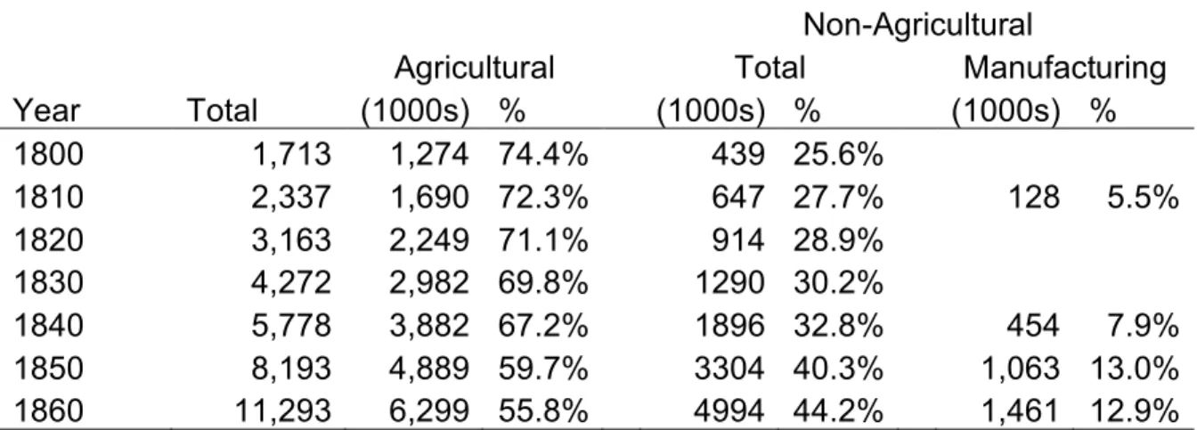
and its distribution in the antebellum era. In 1800, close to three-quarters of the nation’s 1.7 million workers were employed in agriculture. Sixty years later, total agricultural employment had more than quadrupled, but agriculture’s share of employment had fallen to just 55.8 percent of the workforce.
Table 2: U.S. Labor Force, Size and Sectoral Distribution, 1800-1860
Non-Agricultural
Agricultural Total Manufacturing
Year Total (1000s) % (1000s) % (1000s) % 1800 1,713 1,274 74.4% 439 25.6% 1810 2,337 1,690 72.3% 647 27.7% 128 5.5% 1820 3,163 2,249 71.1% 914 28.9% 1830 4,272 2,982 69.8% 1290 30.2% 1840 5,778 3,882 67.2% 1896 32.8% 454 7.9% 1850 8,193 4,889 59.7% 3304 40.3% 1,063 13.0% 1860 11,293 6,299 55.8% 4994 44.2% 1,461 12.9% Notes and Sources: Carter et al (2006), Table Ba 814-830. Division between agriculture and non-agriculture relies on Weiss's labor force series. Manufacturing employment is imputed using the share of manufacturing in non-agricultural employment reported by Lebergott (1964, p. 510).
In 1800, the nation’s manufacturing sector was too small for any data on its size to be available. In 1810, the best estimate is that only about 1 in 20 workers was employed in
manufacturing. Manufacturing employment grew more quickly than the labor force as a whole, however, reaching about 8 percent of the workforce in 1840 and 13 percent by 1850.
By the beginning of the Civil War, the United States was well on the way to becoming the industrial power that it would be in the late nineteenth century. In 1800, however, it was not at all obvious that manufacturing had a future in the country. With abundant land available on the frontier free adult males faced few obstacles to entry into farming, and it was hard to imagine
that industrial wages could rise enough to entice them to give up their independence. More concisely, manufacturers confronted a limited and inelastic supply of labor.
Early efforts to establish factory production in the United States quickly ran up against this shortage of a potential labor supply. However, frictions that slowed the westward migration of New England farmers gave rise to an untapped source of potential factory labor, but one which required a combination of technological and institutional innovations to effectively mobilize. These innovations took shape in New England after 1807, when Jefferson’s embargo and the War of 1812 protected fledgling textile manufacturers from international competition. After the war ended these manufacturers were able to secure the passage of tariff legislation that enabled them to continue to expand, until by the 1830s they had become competitive with British imports.
Labor Supply for the Textile Industry
Beginning in the 1770s a series of mechanical innovations in the spinning and weaving of cotton textiles had transformed the British textile industry giving rise to the Industrial
Revolution. Despite British efforts to prevent the diffusion of these technologies, information about British innovations in spinning cotton crossed the Atlantic quickly in the years after the American Revolution. But the problem of imitating British production extended beyond
acquiring technical knowhow. The scarcity of skilled factory labor, the high costs of capital and the small market for factory produced yarn all posed significant challenges to Americans seeking to establish textile factories.
The most successful efforts at textile production were undertaken by a pair of Providence, Rhode Island merchants, William Almy and Moses Brown, who had successfully recruited a
British mechanic, Samuel Slater, familiar with the construction of the Arkwright water frame. Almy and Brown financed Slater’s construction of a water powered spinning mill based on the Arkwright technology. In contrast to other spinning technologies at the time, operation of the water frame required little skill or strength, and the early factor labor force was made up of 9 children between the ages of 4 and 10 and a single adult supervisor, all recruited from nearby
farms.15 To convert yarn from the mill into fabric, Almy and Brown relied on a network of farm
women who wove the fabric at home.
This model proved financially viable and similar small spinning mills multiplied throughout southern New England. The difficulty of recruiting weavers, however, constrained the growth of these enterprises. Expanding capacity meant distributing yarn over increasingly large areas, and raised both costs and problems of supervision. Without subsequent innovations in both technology and labor supply American textile manufacturing would have remained a small niche industry.
When the Embargo Act and the War of 1812 largely cut off supplies of imported fabric and lowered the cost of raw cotton a number of enterprising New England merchants were prompted to invest in efforts to expand domestic production capacity. The key breakthrough was made by Frances Lowell, who established the Boston Manufacturing Company in 1813.
Lowell’s venture was of an entirely different nature than the small Rhode Island spinning mills. Relying on the use of newly developed water-powered mechanical looms to get around the limited supply of handloom weavers that constrained the Rhode Island Industry, the Boston
Manufacturing Company integrated the entire production process under one roof.16
But this technological solution to the shortage of skilled handloom weavers created a different labor supply problem. The Boston Manufacturing Company factory required a labor
force of several hundred adult workers, far more than could be obtained in the vicinity of the factory. The solution was to expand the scope of the labor market. As Lowell and his partners recognized, the uneven movement of population into the Midwest was giving rise to a significant under-employed workforce throughout rural New England.
In the first half of the nineteenth century, the introduction of steamboats on western rivers, the opening of the Erie Canal, and then construction of major East-West rail links had the effect of raising the returns to commercial agriculture in the Midwest, and encouraging westward migration. If westward migration had been costless, New England might simply have been abandoned as farmers relocated further west onto more productive agricultural land. However, the costs of migration slowed westward movement, while competition in agricultural product markets depressed farm incomes and reduced the resources available to eastern farmers to
finance their relocation.17 The alternative to moving west was to allocate increased amount of
labor in the farm household to non-farm production under putting out arrangements or by moving to the factories. Because young men were disproportionately likely to undertake the expense and risk of westward migration, there was a large surplus of the young unmarried women. Lowell recognized that these women could be tapped to supply his factory and they rapidly became the foundation for an expanding factory workforce. For these young women, the opportunity work in the mills offered a chance to escape depressed agricultural areas and
contribute to their family’s finances or accumulate a dowry while they awaited the opportunity to marry.
To employ these women, Lowell dispatched recruiters to travel through the rural areas of New England offering employment. To house the women once they arrived, he constructed dormitories to house them. Even so, the mills had to offer higher wage rates than they could earn
at home, paying roughly 50 more than they could earn working at home on the manufacture of
palm leaf hats or in smaller mills on the Rhode Island model.18
The combination of technological and labor market innovations introduced by Lowell and Moody proved remarkably successful, and provided the template for the rapid expansion of the textile industry in New England. The Boston Manufacturing Company’s first plant began production in early 1815. Three years later the company began construction of a second plant. Soon after it had exhausted the available water power in Waltham and new mills began to spread to other water power sites in Massachusetts and New Hampshire. By 1850, American textile manufacturing capacity had reached nearly half that of Great Britain, up from less than 2 percent
in 1812.19
By mid-century the growth of manufacturing in New England—not just textiles, but boot and shoe manufacture and other low-tech industries, such as palm leaf hats—was increasingly pressing against labor supply, driving up wages. As Claudia Goldin documents, growing demand caused female earnings to rise relative to males. In 1820, women’s wages were just 30 percent of men’s in manufacturing; by 1840 the ratio had increased to 45 percent and by 1860 it
had risen to over 50 percent.20 Without new sources of labor supply, rising wages would have
slowed the region’s growth. Fortunately, the resolution to this problem came in the form of a rising tide of European immigration.
International Migration
In the first half of the nineteenth century, the United States was, relative to Europe, land-abundant and labor-scarce. As a result, wages in the United States were above those workers could expect to earn in Europe. The high cost of trans-Atlantic passage relative to workers’
incomes restrained migration, however. With the end of the international slave trade in 1808, and the decline of indentured servitude, trans-Atlantic migration slowed. As Figure 4 shows, net migration into the country was relatively modest through the early 1830s. Beginning in the 1830s, however, falling costs of travel began to encourage a growing movement of population, and after the mid-1840s, rates of migration expanded rapidly. By the early 1850s the number of arrivals was more than four times what it had been a decade earlier. The rapid rise in migration reflected largely the effect of events in Europe, primarily the Irish potato famine and political turmoil in Germany, that served to expand the supply of labor.
While the rising supply of potential European migrants was essentially exogenous to the U.S. economy, the destinations these migrants chose within the United States were not.
Disproportionately they gravitated toward the northern part of the country. By 1860, the Census recorded 3.6 million foreign-born whites in a total population of 31.5 million. Only 11 percent of the foreign-born were living in the South, where they made up between 3 and 7 percent of the population. In contrast, more than 20 percent of the Middle Atlantic population at the time was foreign-born, and immigrants made up 15 to 17 percent of the population in other parts of the
Northeast and Midwest.21
Joseph Ferrie examined the mobility of newly arrived European immigrants based on a sample of 2,594 individuals arriving in New York in the 1840s that he linked to their entries in the 1850 and 1860 Census manuscripts. Although most did not remain long in New York City, Ferrie found that more than half gravitated to destinations in New York State, Ohio or
Pennsylvania, primarily in urban areas. Comparing the immigrant sample to a comparable group of the native-born he found that the immigrants were more geographically mobile: almost 70
Fig. 4 Net Immigration to the United States, 1800-1860. Source: Carter et al, Historical
Statistics, series Ad16-20.
0 0.002 0.004 0.006 0.008 0.01 0.012 0.014 0.016 0.018 0 50000 100000 150000 200000 250000 300000 350000 400000 450000 1800 1805 1810 1815 1820 1825 1830 1835 1840 1845 1850 1855 1860 Ax is T itl e
Net Migration and Number of Migrants Relative to Population,
1800-1860
percent had changed counties between the 1850 and 1860 censuses, compared to 43 percent of
comparable linked sample from the native-born population.22
Technological Innovation and the Labor Market
The textile industry was only one of a number of industries in which a distinctive “American system” of manufactures emerged in the first half of the nineteenth century. In the production of locks, clocks, and firearms, as well as textiles, Americans pioneered approaches to manufacturing that in comparison to European industries at the time relied heavily on
mechanization and focused on producing relatively standardized products. The divergent paths of technological innovation on the two sides of the Atlantic have long intrigued economic historians who have sought to link labor market conditions to the direction of technological innovation.
Erwin Rothbarth and H. J. Habakkuk were among the first scholars to attempt to link the direction of American technological innovation to labor supply conditions, arguing that the relative scarcity of labor in the United States encouraged the adoption of capital-intensive (and
by implication, labor-saving) technological innovations.23 Their conjectures have been subjected
to intense scrutiny on both theoretical and empirical grounds.24 Paul David, for example, has
emphasized that their argument is inconsistent with the conventional neo-classical theory of the
firm, but the spirit of their interpretation can be rescued by a more historical argument.25
Empirical investigation has further undermined the capital-labor substitution argument, however, by demonstrating that aggregate capita-labor ratios were actually lower in the United States than
Closer examination of a number of industries suggests that, rather than substitution capital for labor, American innovators sought to develop ways to conserve on traditional craft skills, which were in short supply in the United States. They did this, as the textile industry case suggests, by substituting raw materials and special-purpose machinery, which could be operated by less skilled workers, who were available in greater abundance than those possessing
traditional craft skills.27 One of the chief examples of this substitution is the manufacture of
firearms. In this industry, American manufacturers pursued the production of standardized components that could be assembled without the custom-fitting common in Britain, first by developing systematic techniques of measurement and then by introducing a range of special purpose machinery that made it possible to produce guns without the all-round craft skills of
British gunsmiths.28
Markets for Agricultural Labor
Throughout the Antebellum period, the bulk of the U.S. labor force was employed in agriculture. At first glance the labor market model sketched in section 2 would seem to have little relevance for the allocation of agricultural labor. The majority of farms were owner operated and relied primarily on family labor. In the northern states, virtually all farms were under 500 acres in size. Young men seeking to accumulate funds to go into farming did provide a supply of potential hired help, but by one estimate there was on average just one hired male
worker for every two farms.29
The limited use of hired labor was, however, itself a reflection of labor market
conditions. The supply of agricultural labor was scarce and unreliable, conditions that made it unattractive for most farmers to rely on hired labor and prompted them to limit their farms to a
scale they could manage with family labor. Except near cities, few farmers could count on being able to reliably hire help when they needed it. Demands for harvest labor occurred in a short window, and competition for the scarce supply of potential workers drove up wages. Moreover, the transitory nature of employment meant that neither farmers nor farm laborers were willing to make long-term commitments. As in other sectors, labor supply conditions exerted an influence on technological innovation. According to Paul David scarce and inelastic supplies of
agricultural labor were an important factor encouraging the rapid adoption of mechanical reapers
in the Midwest in the 1840s.30
The role of labor scarcity in constraining northern farm sizes is confirmed by comparison with the South. In the South, the existence of well-developed markets for slaves—both for purchase and short term hiring—allowed planters to expand their farms well beyond the scale that could be cultivated with family labor. In some areas of the south planters employed 50 or more slaves and farmed thousands of acres. Slaves were expensive, however, and slave ownership became increasingly concentrated. In 1860, less than one-third of southern farms
owned any slaves.31
Although much agricultural labor was provided by owner-operators or their family members, decisions to enter or remain in agriculture all took place in the context of the non-agricultural employment opportunities. More or less explicitly, those in the non-agricultural sector chose this employment over the alternative of entering the non-agricultural labor market. The attractiveness of the agricultural sector was thus a key determinant of the supply of non-agricultural labor.
Even though the share of labor employed in agriculture was declining in the antebellum period, in absolute terms the agricultural sector experienced considerable growth. Frontier
farming offered opportunities for wealth accumulation, and allowed farmers to monetize their time and that of their family more effectively than urban employment. But entry into agriculture was costly, preventing most immigrants and urban laborers from moving into farming. Land on the frontier was relatively plentiful and cheap, but clearing land, building structures and fences, and purchasing supplies and implements was costly. According to one hypothetical calculation by the State of Minnesota, in 1860 the cost of establishing a 160-acre farm was $795,
approximately 5 times the annual earnings of a farm laborer at the time.32 As a result, the
majority of farmers were drawn from the existing agricultural population.
Antebellum Wages
In the labor market model sketched in section 2, wages are the price of labor. In equilibrium, the wage is determined by the interaction of supply and demand. Between
American Independence and the Civil War labor markets were obliged to respond to a range of shocks to supply and demand. Transportation improvements opened vast areas of productive farmland, raising the returns to agriculture and creating new economic opportunities in the trans-Alleghany west. Technological innovations in the production of textiles, and he development of new methods of precision manufacturing raised the productivity of labor manufacturing and encouraged the emergence of an urban factory labor force. Falling costs of trans-Atlantic passage combined with shocks to European labor encouraged a rising tide of immigration. The dynamism of the American economy in the antebellum period reflected the ability of the labor market to respond to these and other shocks, facilitating the movement of labor toward its highest value uses. The behavior of wages provides a more precise indication of just how efficiently this reallocation was accomplished.
Spatial Integration
As the data in Table 2 illustrate, over the antebellum period population growth was combined with a substantial geographic redistribution from East to West. In terms of the labor market model sketched above, the movement of labor and population reflects a labor supply response to greater economic opportunity—i.e., higher wages—on the frontier. Although nominal rates of pay in the Midwest appear to have been lower than in the Northeast, adjusting
for regional differences in the cost of living reveals a real wage advantage for the Midwest. 33 In
addition to the opportunity to increase pay within any occupation migrants are likely to have been motivated to move by opportunities to move up the occupational ladder that were available in regions of recent settlement. Using a sample of individuals linked across census years, Laura Salisbury found that individuals who changed counties between census years were more likely to move to locations where skill premiums were higher, evidence consistent with the hypothesis
that opportunities for occupational upgrading were a factor motivating their migration decision.34
The labor market model suggests that over time the labor supply response to geographic
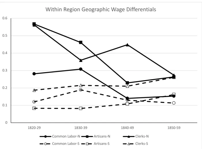
wage differentials should, other things equal, result in a narrowing of regional wage differentials, and this prediction appears to be borne out by the available evidence. Using data collected from payroll records of the U.S. military that report wages paid to civilian workers at military forts located throughout the country Robert Margo has been able to reconstruct time trends of real
wages by region from 1820 through 1860. 35 Figure 5 shows the evolution of East-West wage
differentials for three different occupations – unskilled common labor, artisans, and white collar workers – separately in the northern and southern parts of the country. Because of slavery,
Fig. 5. West-East Wage Differentials by Occupation and Region, 1820-1860. Notes and sources: Dashed lines show wage differentials between the South Central and South Atlantic Regions; solid lines show wage differentials between the North Central and Northeast regions. Margo,
Wages, pp. 104-5. 0 0.1 0.2 0.3 0.4 0.5 0.6 1820-29 1830-39 1840-49 1850-59
Within Region Geographic Wage Differentials
Common Labor-N Artisans-N Clerks-N
Northern and Southern labor markets were largely isolated from one another, and the central question is how effective markets were within each group of states in reallocating labor.
The behavior of inter-regional wage differentials was quite different In the North and South, however. In the North, in the 1820s the regional wage gaps for skilled artisans and white collar workers were far higher (on the order of 60 percent) than for common laborers (a little less than 30 percent). Perhaps reflecting the effects of slavery in facilitating westward migration in the South, all of the regional wage differentials were much smaller in the South. As time progressed, however, it is apparent that wage differentials in the North narrowed substantially, dropping by more than 50 percent. By the 1850s, the regional wage gap for common labor was only about 15 percent, while the gap for more skilled labor had fallen to below 30 percent. Thus, labor markets were successful in reducing but not entirely eliminating regional wage
differentials.
Additional evidence of the effectiveness of antebellum labor markets is provided by the extreme shock of the California Gold Rush. The discovery of gold in California in 1848 is an example of an unpredictable labor demand shock. The rapid influx of labor in response is one manifestation of labor market integration. Robert Margo has examined the labor market response of the gold rush in detail and estimates that while the very short run response to the gold discovery was highly inelastic, over the course of the next few years labor supply became
much more elastic.36
Inter-sectoral Integration
In addition to facilitating inter-regional movements of labor, the growth of manufacturing required labor markets to shift labor between different sectors. The antebellum period was
characterized by the growing importance of manufacturing, which required shifting resources from agriculture to industry, and from rural to urban places. The labor market model suggests that the size of wage gaps between sectors is a reflection of how effectively labor markets shifted labor between sectors. Although the evidence is incomplete, labor markets appear to have been
quite efficient in accomplishing inter-sectoral redistribution of labor.37
Measures of average output per worker point to the higher productivity of
non-agricultural labor. According to Thomas Weiss, gross product per non-non-agricultural worker—that is, the value of all goods and services produced by the non-agricultural sector—was 2.3 times as
great as gross product per worker in agriculture.38 Of course, this measure fails to capture capital
gains that farmers earned from investments in land clearing, so the gap in returns to labor was presumably much smaller. Ideally, we would want to compare wages that a worker could earn in agricultural and non-agricultural employments. However, the data needed for this comparison are not available for most of the antebellum period. In 1850 and 1860, however, the U.S. Census of Social Statistics began to report county level wages for a variety of occupations. Comparisons are complicated by differences in the geographic location of farm and non-farm jobs as well as differences in the terms of employment in the two sectors. Farm labor wages, for example, were mostly reported for monthly contracts, while manufacturing wages were often daily wages, making it necessary to adjust for both the number of days actually worked and for the greater risks of unemployment faced by manufacturing workers.
Robert Margo has carefully adjusted agricultural and non-agricultural wage data from the 1850 and 1860 Censuses to make them as comparable as possible. He found that within counties the gaps between farm and non-farm wages were quite small on average. When differences are considered at the state level, the gaps were larger, but much of this is attributable to differences
in the location of agricultural and non-agricultural workers. Non-agricultural labor was more likely to live in urban areas with higher living costs. Adjusting for these differences it appears that gaps in real wages were relatively small, indicating that the movement of labor supply between sectors was effective in integrating markets for the two sectors.
The Growth of Real Wages
The antebellum period marked the beginning of sustained economic growth. Between 1800 and 1860 Real GDP per capita increased by 87 percent, rising from $1,509 to $2,815 in
2009 prices.39 Because labor force participation was increasing, some of the growth in
production per capita reflected a rise in labor input. Adjusting for the increase in labor input, GDP per worker increased by roughly 60 percent between 1800 and 1860, with virtually all of
the increase concentrated after 1820.40
Figure 6 plots the trend in real wages for common labor, artisans and clerks during the antebellum period. Before the 1820s consistent time series of wages are quite limited, and the common labor series is based on wages in Philadelphia and non-farm workers in Massachusetts. Beginning in the 1820s data on a more representative national scale become available from the
records paid to civilian workers employed at U.S. military forts throughout the country.41 Before
the mid-1820s common labor wages fluctuated with little clear trend. Beginning in the 1820s, however, real wages for all three categories of workers began to rise. According to Robert Margo the growth of real wages between 1820 and 1860 grew at the same rate as GDP per worker, indicating that in the long run the benefits of the nation’s economic growth were passed
Fig. 6. Real Wages, 1800-1860, by Occupation. Sources: Common Labor (David-Solar) - Lawrence H. Officer and Samuel H. Williamson, “Annual Wages in the United States,
1774-Present,” MeasuringWorth, 2017 https://www.measuringworth.com/uswage/ (accessed
10/8/2017); other series – Carter et al, Historical Statistics, Series Ba4267-4353.
0 20 40 60 80 100 120 140 160 180 200 1800 1805 1810 1815 1820 1825 1830 1835 1840 1845 1850 1855 1860 Rea l W age In dex (1830=100)
Real Wages, 1800-1860
Over shorter periods of time Figure 6 suggests that the behavior of real wages could be quite volatile. For example, after rising by about 30 percent from the 1820s to the mid-1830s, common labor wages fell by almost half that amount between 1837 and 1840. They rose again in the early 1840s and before dropping sharply after 1844. Such short run fluctuations must have made it much harder for workers to perceive the effects of more gradual long-run improvements in wages on their purchasing power. Although living standards in the antebellum United States compared favorably to those of other countries at the time and were improving it is worth recalling that the mass of laboring people worked long hours at physically demanding jobs
for what would today seem very modest rewards.43
Skill Differentials
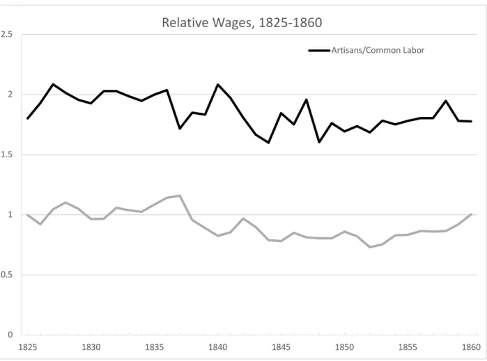
Although wages increased for all three categories of workers represented in Figure 6, growth rates varied across the different skill groups. In particular, wages grew more slowly for artisans than they did for either unskilled common labor or for white collar labor, represented by clerks. These trends are illustrated in Figure 7, which plots the wages of artisans relative to each of these groups of workers.
The labor market model suggests that wage growth reflects the relative shifts of supply and demand over time. That the wages of artisans grew more slowly (relative to supply) than those of common laborers is consistent with the view that technological changes associated with the spread of factory production slowed the growth of demand for skilled artisanal labor relative to that for less skilled factory workers. On the other hand, the rising relative wage of clerks
Fig. 7.Relative Occupational Wages, 1825-1860. Source: Margo, Wages, pp. 104-5. 0 0.5 1 1.5 2 2.5 1825 1830 1835 1840 1845 1850 1855 1860
Relative Wages, 1825-1860
Artisans/Common Laborsuggests that technological changes in the antebellum economy helped to boost demand for
skilled white-collar workers along with that for the unskilled.44
Conclusion
Labor is an essential factor in the production of goods and services in an economy. The central function of labor markets is to allocate labor toward its most productive uses. In the years between American independence and the Civil War, rapid population growth, westward expansion, and the beginning of industrialization required the mobilization of labor
geographically and between sectors. The dynamism of the economy in this period is a reflection of the effectiveness of labor markets in accomplishing this redistribution.
Yet the history of antebellum labor markets is more complex than this. The division of the nation between regions that permitted and outlawed slavery reshaped understanding of labor market transactions, giving rise to a unique conception of the meaning of free labor, defined in contrast to slavery. Differences in property rights regimes shaped regional investment strategies and created persistent differences in the nature of regional development strategies. At the same time, labor market imperfections played an important role in creating the labor force that early manufacturing enterprises required to be competitive. Had northern labor markets been more efficient, more of the population of rural New England would have moved west, depriving manufacturers of the workers they needed to staff their factories.
Discussion of the Literature
The history of antebellum U.S. labor market rests on a foundation of quantitative
of the size and sectoral distribution of the labor force in the early 1960s.45 These have
subsequently been refined by Thomas Weiss.46 A number of scholars have contributed to
knowledge about the behavior of wages over time and in different sectors and occupations
through difficult archival work.47 The most comprehensive effort to collect and analyze wage
data in the antebellum period was conducted by Robert Margo who gathered data from wages
paid by the U.S. military to civilian contractors at forts throughout the country.48 Much of the
most useful statistical evidence on labor markets is collected in Historical Statistics of the United
States, Millennial Edition, which includes extensive discussion of data sources as well as
valuable interpretive essays.49
The emergence and expansion of factory production and the attendant growth in the factory labor force is one of the central themes of antebellum labor markets. Much can be learned about the early industrial labor force and its recruitment from histories of the textile
industry.50 One of the central issues in this history concerns the effects of labor supply on the
location of factories. A number of different studies have suggested slightly different pathways
connecting labor supply conditions to factory location.51 The transition from artisanal shops to
factories, and the growth in the size and complexity of factory production entailed transitions in
the social relations of labor and capital that have been explored labor and social historians.52
Market exchange is premised on the ability of buyers and sellers to clearly describe the goods or services being exchanged and to transfer ownership or control in exchange for monetary payments. Market participants also need to have some recourse to resolve conflicts that arise in relation to these transactions. A number of recent studies have examined the
particular importance for the history of antebellum labor markets are the consequences of
slavery.54
Immigration to the United States exerted an important influence on labor markets, especially after the early 1840s. Much of the literature on the causes and consequences of immigration focuses on the postbellum period. But there are a number of useful studies that
focus on or include the pre-Civil War era.55
Primary Sources and Digital Material
Given the breadth of topics encompassed under the rubric of antebellum labor markets primary source materials are quite diverse and varied. For those seeking quantitative evidence
on wages, population, immigration, and the labor force the best place to begin is with Historical
Statistics of the United States. Volume 2 of this collection includes a wealth of primary data on
work and welfare as well as citations to original sources.56 The early history of manufacturing in
New England is well documented. The University of Massachusetts Lowell has digitized letters written by some of the young women who worked in the early textile factories, as well as a
monthly magazine, the Lowell Offering, that was written and published by women working in the
textile mills.57 There are also collections of material relating to shoemaking, another early
industry that emerged in New England in the antebellum era.58 Federal Population censuses offer
a wealth of social and economic information relevant to the history of antebellum labor markets. Students seeking to explore this information can access them in a variety of ways. The
Minnesota Population Center at the University of Minnesota has compiled machine readable
samples from the population censuses beginning in 1850.59 The Ancestry.com website offers
search engine.60 A number of useful representations of census data can viewed through tools
available on the socialexplorer.com website.61
Further Reading
Ferrie, Joseph P. Yankeys Now: Immigrants in the Antebellum United States (New York, 1999).
Field, Alex James. “Sectoral Shifts in Antebellum Massachusetts: A Reconsideration.”
Explorations in Economic History 15 (1978), 146-71.
Goldin, Claudia D. Understanding the Gender Gap: An Economic History of American Women
(New York, 1990).
Gordon, David M., Richard Edwards and Michael Reich Segmented Work, Divided Workers: The
Historical Transformation of Labor in the United States (Cambridge, 1982).
Gutman, Herbert. “Work, Culture, and Society in Industrializing America 1815-1919.” American
Historical Review 78 (1973), 531-88.
Lebergott, Stanley. Manpower in Economic Growth: The American Record since 1800 (New
York, 1964)
Margo, Robert A. Wages and Labor Markets in the United States, 1820-1860 Chicago, 2000).
Margo, Robert A. “Labor Markets.” In Handbook of Cliometrics, Claude Diebolt and Michael
Haupert, eds. (Berlin, 2014).
Rosenbloom, Joshua L. “The History of American Labor Market Institutions and Outcomes.” EH.Net Encyclopedia. Robert Whaples, ed. (Eh.Net, 2008)
http://eh.net/encyclopedia/the-history-of-american-labor-market-institutions-and-outcomes/ (Accessed 9/21/2017).
Rosenbloom, Joshua L. “Path Dependence and the Origins of Cotton Textile Manufacturing in
New England.” In David Jeremy and Douglas A. Farnie, eds. The Fibre that Changed the
World: Cotton Industry in International Perspective (Oxford, 2004)
Rosenbloom, Joshua L. And William A. Sundstrom. “Labor-Market Regimes in U.S. Economic
History.” In Economic Revolutions in Historical Time. Paul W. Rhode, Joshua L.
Rosenbloom and David F. Weiman, eds. (Stanford, 2011).
Steinfield, Robert J. The Invention of Free Labor: The Employment Relations in English and
American Law and Culture, 1350-1870 (Chapel Hill, 1991)
Wright, Gavin. Slavery and American Economic Development (Baton Rouge, 2006).
Notes
1Joshua L. Rosenbloom, “The History of American Labor Market Institutions and Outcomes,” in
EH.Net Encyclopedia, Robert Whaples, ed. (2008),
http://eh.net/encyclopedia/the-history-of-american-labor-market-institutions-and-outcomes/ (accessed 9/21/2017).
2 David Galenson, White Servitude in Colonial America (New York, 1981).
3 Robert J. Steinfeld, The Invention of Free Labor: The Employment Relationship in English and
American Law and Culture, 135-1870, (Chapel Hill, 1991), chs. 1-2; Joshua L. Rosenbloom and
William A. Sundstrom, “Labor Market Regimes in U.S. Economic History,” in Economic
Revolutions in Historical Time, Paul W. Rhode, Joshua L. Rosenbloom and David F. Weiman, eds. (Stanford, 2011), pp. 283-84.
4 Peter Kolchin, American Slavery, 1619-1877 (New York, 1993), pp. 63-70.
5 Quoted in Gavin Wright, Slavery and American Economic Development (Baton Rouge, 2006),
p. 49.
6 Wright, Slavery, pp. 41-46.
7 Steinfeld, Invention, pp. 147-72.
8 Wright, Slavery, ch. 2; Gavin Wright, Old South, New South: Revolutions in the Southern
Economy Since the Civil War (New York, 1986), pp. 17-50; Fred Bateman and Thomas Weiss, A Deplorable Scarcity: The Failure of Industrialization in the Slave Economy (Chapel Hill, 1981).
9 Robert W. Fogel, Without Consent or Contract: The Rise and Fall of American Slavery (New
York, 1989), pp. 89-92; Edward Baptist, The Half Has Never Been Told: Slavery and the Making
of American Capitalism (New York, 2014), pp. 173-79; Jonathan B. Pritchett, “Quantitative
Estimates of the United States Interregional Slave Trade, 1820-1860,” Journal of Economic
History 61 (2001), pp. 467-75.
11 Alan L. Olmstead and Paul W. Rhode, “Biological Innovation and Productivity Growth in the
Antebellum Cotton Economy,” Journal of Economic History 68 (2008), pp. 1123-71.
12 Gavin Wright, Political Economy of the Cotton South: Households, Markets and Wealth in the
Nineteenth Century (New York, 1978), ch. 139-50.
13Charles W. Calomiris and Jonathan Pritchett, “Betting on Secession: Quantifying Political
Events Surrounding Slavery and the Civil War.” American Economic Review 106 (2013), pp.
1-23.
14 David M. Gordon, Richard Edwards and Michael Reich, Segmented Work, Divided Workers:
The Historical Transformation of Labor in the United States (Cambridge, 1982), p. 48.
15 Joshua L. Rosenbloom, “Path Dependence and the Origins of Cotton Textile Manufacturing in
New England,” in The Fibre that Changed the World: The Cotton Industry in International
Perspective, 1600-1990s, Douglas A. Farnie and David J. Jeremy, eds. (Oxford, 2004), p. 371.
16 Rosenbloom, “Path Dependence,” pp. 375-80.
17 Alex James Field, “Sectoral Shifts in Antebellum Massachusetts: A Reconsideration,”
Explorations in Economic History 15 (1978), pp. 146-71.
18 Stanley Lebergott, “Wage Trends, 1800-1900,” in Trends in the American Economy in the
Nineteenth Century, National Bureau of Economic Research, Conference on Research in Income and Wealth (Princeton, 1960), p. 451.
19 Rosenbloom, “Path Dependence,” p. 366.
20 Claudia D. Goldin, Understanding the Gender Gap: An Economic History of American
Women (New York, 1990), p. 62.
21 Susan B. Carter, Scott Sigmund Gartner, Michael R. Haines, Alan L. Olmstead, Richard Sutch
and Gavin Wright, eds., Historical Statistics of the United States: Earliest Times to the Present,
Millenial Edition (New York, 2006), vol. 1, series Aa2244-6550.
22Joseph P. Ferrie, Yankeys Now: Immigrants in the Antebellum U.S., 1840-1860 (New York,
1999).
23 Erwin Rothbarth, “Causes of the Superior Efficiency of U.S.A. Industry as Compared to
British Industry,” Economic Journal 56 (1946), pp. 383-90; H. J. Habakkuk, American and
British Technology in the Nineteenth Century: The Search for Labour-Saving Inventions
(Cambridge, 1972).
24 Peter Temin, “Labor Scarcity and the Problem of American Industrial Efficiency in the 1850s”
Journal of Economic History 26 (1966), pp. 277-98.
25 Paul A. David, Technical Choice, Innovation and Economic Growth: Essays on American and
British Experience in the Nineteenth Century (London, 1975), ch. 1.
26 Alex James Field, “Land Abundance, Interest/Profit Rates, and Nineteenth-Century American
and British Technology,” Journal of Economic History 43 (1983), pp. 405-31; John A. James
and Jonathan S. Skinner, “The Resolution of the Labor-Scarcity Paradox,” Journal of Economic
History 45 (1985), pp. 513-40.
27 Edward Ames and Nathan Rosenberg, “The Enfield Arsenal in Theory and History,”
Economic Journal 78 (1968), pp. 827-42; Nathan Rosenberg, Perspectives on Technology (New York, 1976), ch. 3.
28 Joshua L. Rosenbloom, “Anglo-American Technological Differences in Small Arms
29 Jonathan Hughes and Louis P. Cain, American Economic History, 8th edition (Boston, 2011), p. 174.
30 David, Technical Choice, ch. 4.
31 Wright, Political Economy, ch. 2.
32 Minnesota Commissioner of Statistics, Minnesota: Its Place Among the States Being the First
Annual Report of the Commissioner of Statistics (Hartford, 1860), p. 88.
33 Philip Coelho and James Shepherd, “Regional Differences in Real Wages: The United States,
1851-1880,” Explorations in Economic History 13 (1976), 203-30; Robert A. Margo, “Regional
Wage Gaps and the Settlement of the Midwest,” Explorations in Economic History 36 (1999),
pp. 128-43. Richard Easterlin’s estimates of regional per capita income, which did not adjust for differences in regional cost of living, show that per capita income was higher in the Northeast than the Midwest, “Interregional Differences in Per Capita Income, Population, and Total Income, 1840-1950,” in Trends in the American Economy in the Nineteenth Century, National Bureau of Economic Research, Conference on Research in Income and Wealth (Princeton, 1960), p. 137
34 Laura Salisbury, “Selective Migration, Wages and Occupational Mobility in Nineteenth
Century America,” Explorations in Economic History 53 (2014), pp. 40-63.
35 Robert A. Margo, Wages and Labor Markets in the United States, 1820-1860 (Chicago, 2000).
36Wages and Labor Markets, ch. 6.
37 Margo, Wages and Labor Markets, ch. 4.
38 “Economic Growth Before 1860: Revised Conjectures,” in American Economic Development
in Historical Perspective, Thomas Weiss and Donald Schaefer, eds. (Stanford, 1994), p. 19.
39 Louis Johnston and Samuel H. Williamson, “What was the U.S. GDP Then?” Measuring
Worth (2017) http://www.measuringworth.org/usgdp/ (accessed 9/22/2017).
40 Weiss, “Economic Growth,” p. 19.
41 See the discussion of data sources in Robert A. Margo “Wages and Wage
Inequality,” in Historical Statistics of the United States, Earliest Times to the Present: Millennial
Edition, Susan B. Carter et al, eds. (New York, 2006), vol. 2, pp. 40-46.
42 Margo, Wages and Labor Markets, p. 143
43 See, for example, the investigation of working class labor in Baltimore before the Civil War in
Seth Rockman, Scraping By: Wage Labor, Slavery, and Survival in Early Baltimore (Baltimore,
2009).
44 Margo, Wages and Labor Markets, pp. 155-56.
45Stanley Lebergott, “Labor Force and Employment, 1800-1960,” in Output, Employment and
Productivity in the United States after 1800, Dorothy S. Brady, ed., National Bureau of Economic Research, Studies in Income and Wealth, no. 30 (New York, 1966).
46 Thomas Weiss, “Revised Estimates of the United States Workforce, 1800-1860,” in
Long-Term Factors in American Economic Growth, Stanley L. Engerman and Robert E. Gallman, eds, Studies in Income and Wealth, no. 51, National Bureau of Economic Research (Chicago, 1986).
47 Stanley Lebergott, Manpower in Economic Growth: The American Record since 1800 (New
York 1964). Donald Adams, “Wage Rates in the Early National Period: Philadelphia,
1785-1830,” Journal of Economic History 28 (1968), 404-26; “Some Evidence on English and
American Wage Rates, 1790-1830,” Journal of Economic History 30 (1970), 499-520; “Prices