Expanding Self-organizing Map for Data
Visualization and Cluster Analysis
Huidong Jin
a,b, Wing-Ho Shum
a, Kwong-Sak Leung
a,
Man-Leung Wong
caDepartment of Computer Science and Engineering, The Chinese University of Hong Kong, Shatin, Hong Kong.
bCSIRO, Mathematical & Information Sciences, Canberra, Australia. cDepartment of Computing and Decision Sciences, Lingnan University, Tuen
Mun, Hong Kong.
Abstract
The Self-Organizing Map (SOM) is a powerful tool in the exploratory phase of data mining. It is capable of projecting high-dimensional data onto a regular, usually 2-dimensional grid of neurons with good neighborhood preservation between two spaces. However, due to the dimensional conflict, the neighborhood preservation cannot always lead to perfect topology preservation. In this paper, we establish an Expanding SOM (ESOM) to preserve better topology between the two spaces. Besides the neighborhood relationship, our ESOM can detect and preserve an or-dering relationship using an expanding mechanism. The computation complexity of the ESOM is comparable with that of the SOM. Our experiment results demon-strate that the ESOM constructs better mappings than the classic SOM, especially, in terms of the topological error. Furthermore, clustering results generated by the ESOM are more accurate than those obtained by the SOM.
Key words: Self-organizing map, neural networks, data mining, visualization, clustering analysis.
1 Introduction
The Self-Organizing Map (SOM) has been proven to be useful as visualiza-tion and data exploratory analysis tools [6]. It maps high-dimensional data items onto a low-dimensional grid of neurons. The regular grid can be used as a convenient visualization surface for showing different features of data such as the cluster tendencies of the data [8, 12, 16]. SOMs have been suc-cessfully applied in various engineering applications covering areas such as pattern recognition, full-text and image analysis, vector quantization, regres-sion, financial data analysis, traveling salesman problem, and fault diagnosis [3, 4, 6, 7, 10, 14, 18].
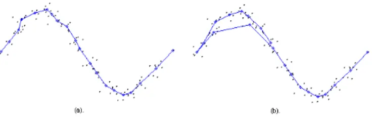
However, because a SOM maps the data from a high-dimensional space to a low-dimensional space which is usually 2-dimensional, a dimensional conflict may occur and a perfect topology preserving mapping may not be generated [1, 5]. For example, consider the two trained SOMs depicted in Fig.1, although they preserve good neighborhood relationships, the SOM depicted in Fig.1(b) folds the neuron string onto data irregularly and loses much topology infor-mation in comparison with the SOM shown in Fig.1(a).
There are many research efforts to enhance SOMs for visualization and cluster analysis. Most of them focus on how to visualize neurons clearly and classify data [3, 14, 16]. Some work has concentrated on better topology preservation. Kirk and Zurada [5] trained their SOM to minimize the quantization error in
Fig. 1. Two SOMs from 2-dimensional space to 1-dimension. The connected dots indicate a string of neurons, and other dots indicate data.
the first phase and then minimize the topological error in the second phase. Su and Chang proposed a Double SOM (DSOM) that uses a dynamic grid structure instead of a static structure used in the conventional SOMs. The DSOM uses the classic SOM learning rule to learn a grid structure from input data [12].
Motivated by an irregularity problem of SOMs and our previous work of using SOM for traveling salesman problem [4], we propose a new learning rule to enhance the topology preservation. The paper is organized as follows. We outline the SOM techniques in the next section. We introduce our ESOM in Section 3, followed by its theoretic analysis. The visualization and clustering results of the ESOM are presented and compared with the SOM in Section 4. A conclusion is given in the last section.
2 Self-Organizing Map
The SOM consists of two layers of neurons. The neurons on the input layer receive data ~xk(t) = [x1k(t), x2k(t),· · · , xDk(t)]T ∈ <D (1 ≤ k ≤ N) at time
t where D is the dimensionality of the data space and N is the number of data items in the data set. The neurons on the output layer are located on a grid with certain neighborhood relationship. In this paper, the rectangular
neighborhood is used. The weight vector w~j(t) = [w1j(t), w2j(t),· · · , wDj(t)]T
∈ <D (1 ≤ j ≤ M) indicates the j-th output neuron’s location in the data
space. It moves closer to the input vector according to
~
wj(t+ 1) =w~j(t) +²(t)hj,m(t)[~xk(t)−w~j(t)]. (1)
Herem(t) is the winning neuron,hj,m(t) isthe neighborhood function, and²(t)
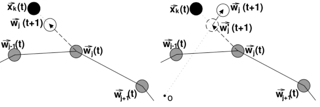
isthe learning rate and usually shrinks to zero. Fig.(2)(a) illustrates this learn-ing rule. Durlearn-ing the learnlearn-ing, the SOM behaves like a flexible net that folds onto the “cloud” formed by the input data. It finally constructs a neighbor-hood preserving map so that the neurons adjacent on the grid have similar weight vectors. The SOM usually maps a high-dimensional data set to a low-dimensional grid, so a low-dimensional conflict may occur in the trained SOM. Thus, the neighborhood preserving map of the SOM is a good but usually not a perfect topology preserving one.
3 Expanding SOM
Besides the neighborhood relationship in the SOM, another topology relation-ship can be detected and preserved during the learning process to achieve a better topology preserving mapping for data visualization. This is a linear ordering relationship based on the distance between data and their center. A neural network can detect and preserve this ordering relationship. If the tance between a data item and the center of all data items is larger, the dis-tance between the corresponding output neuron and the center is also larger. The linear ordering relationship contains certain important topological infor-mation. A typical example may be found in Fig.1. Though two SOMs in Fig.1
(a) and (b) have similar quantization errors, the left one certainly has less topological error. In other words, the left one visualizes the data set better.
In order to overcome such irregularity as in Fig.1(b), we proposed the Expand-ing SOM (ESOM) to learn the linear orderExpand-ing through expandExpand-ing. The ESOM can construct a mapping that preserves both the neighborhood and the or-dering relationships. Since this mapping preserves more topology information of the input data, better performance in visualization can be expected.
We introduce a new learning rule to learn the linear ordering relationship. Different from the SOM, the learning rule of the ESOM has an additional factor, the expanding coefficient cj(t), which is used to push neurons away
from the center of all data items during the learning process. In other words, the flexible neuron network is expanding gradually in our ESOM algorithm. Moreover, the expanding force is specified according to the ordering of the data items. In general, the larger the distance between the corresponding data item and the center is, the larger the expanding coefficient cj(t) is, the larger
the distance between the corresponding data item and the center, the larger the expanding coefficientcj(t). Consequently, the associated output neuron is
pushed away from the center and the ordering of data items is thus preserved in the output neurons. For example, the good topological preserving map in Fig. 1(a) can be achieved.
In the following sub-sections, the ESOM algorithm will be discussed first. Theoretical analysis of the ESOM algorithm will then be described.
3.1 The ESOM algorithm
The ESOM algorithm consists of 6 steps. (1) Linearly transform the coordinates ~x0i = [x0
1i, x02i,· · · , xDi0 ]T (i= 1,· · · , N)
of all given data items so that they lie within a sphere SR centered at the
origin with radius R (<1). Here N is the number of data items, D is the dimensionality of the data set. Hereafter, [x1i, x2i,· · · , xDi]T denotes the
new coordinate of~xi. Let the center of all data items be ~x
0 C = N1 N P i=1~x 0 i and
the maximum distance of data from the data center be Dmax, then
~xi =
R Dmax
³
~x0i−~x0C´ for all i. (2)
(2) Set t = 0, and the initialize weight vectors w~j(0) (j = 1,· · ·, M) with
random values within the above sphereSRwhereM is the number of output
neurons.
(3) Select a data item at random, say~xk(t) = [x1k, x2k,· · · , xDk]T, and feed it
to the input neurons.
(4) Find the winning output neuron, say m(t), nearest to ~xk(t) according to
the Euclidean metric:
m(t) = arg min
j k~xk(t)−w~j(t)k. (3)
(5) Train neuron m(t) and its neighbors by using the following formula:
~ wj(t+ 1) =cj(t)w~ 0 j(t+ 1) 4 =cj(t){w~j(t) +αj(t) [~xk(t)−w~j(t)]} (4)
The parameters include:
• the interim neuron w~0j(t+ 1), which indicates the position of the excited neuronw~j(t) after moving towards the input data item ~xk(t);
• the learning parameter αj(t)(∈ [0,1]), which is specified by a learning
rate ²(t) and a neighborhood functionhj,m(t)(σ(t)):
αj(t) = ²(t)×hj,m(t)(σ(t)); (5)
• the expanding coefficient cj(t), which is specified according to
cj(t) = [1−2αj(t) (1−αj(t))κj(t)]− 1 2 , (6) whereκj(t) is specified by κj(t) = 1− h~xk(t), ~wj(t)i − q (1− k~xk(t)k2)(1− kw~j(t)k2) (7)
(6) Update the neighbor width parameter σ(t) and the learning parameters
²(t) with predetermined decreasing schemes. If the learning loop does not reach a predetermined number, go to Step 3 with t:=t+ 1.
The first step facilitates the realization of the expanding coefficientcj(t). After
the transformation, we can use the norm of a data item k~xk(t)k to represent
its distance from the center of the transformed data items since the center is the origin. Thus, the norm k~xk(t)k can indicate the ordering topology in the
data space. This ordering will be detected and preserved in kw~j(t)k through
the expanding process.
The learning rule defined in Eq.(4) is the key point of the proposed ESOM algorithm. Different from the SOM learning rule, it has an additional multi-plication factor — the expanding coefficient cj(t). This expanding coefficient
is greatly motivated by our work of applying SOM to the traveling salesman problem [4], where the expanding coefficient is defined in a 2-D space by virtue of a unit sphere. Extending the formula for the 2-D case into aD-dimensional space, we get Eq.(4).
It is worth pointing out that, although the expanding coefficient cj(t) is
rel-evant to all data items, the calculation of cj(t) only depends on αj(t), ~xk(t)
and w~j(t). If cj(t) is a constant 1.0, the ESOM is simplified to a conventional
SOM. Since cj(t) is always greater than or equal to 1.0, the expanding force
pushes the excited neuron away from the center. In other words, the inequality
kw~j(t+ 1)k ≥ ° ° °w~0j(t+ 1) ° °
° is always true. Fig.2(b) illustrates the expanding
functionality. After moving the excited neuron w~j(t) towards the input data
item ~xk(t), as indicated by w~0j(t+ 1), the neuron is then pushed away from
the center. So, during the learning process, the flexible neuron net is expand-ing in the data space. More interestexpand-ingly, as the expandexpand-ing force is specified accordingly to the ordering relationships, distant data items are likely to be mapped to the distant neurons, while data items near the center are likely to be mapped to the neurons near the center of map, therefore, cj(t) can help
us to detect and preserve the ordering relationship. The expanding coefficient
cj(t) is also close to 1, which enables the ESOM to learn and preserve the
neighborhood relationship as the SOM does. We will give a theoretical anal-ysis on this point in the next subsection.
There are several variations of SOM for better topology preservation, but most of them are either computationally expensive or structurally compli-cated. GSOM [11] needs to expand its output neuron layer gradually during learning. However, the expansion of ESOM only happens on the output neu-rons’ weight vectors, rather than the structure of output neuron layer. Besides finding the nearest neuron for the input data item as in ESOM/SOM, GSOM also needs to determine whether, where, and how a new output neuron has to be inserted. The two-stage SOM [5] uses both a k-means algorithm and a par-tition error based heuristic to improve the topography preservation. However,
xk(t) (t) j-1 w j+1(t) w wj(t) j(t+1) w o xk(t) (t) j-1 w j+1(t) w wj(t) j(t+1) w' j(t+1) w
Fig. 2. A schematic view of two different learning rules. (a). The learning rule for the traditional SOM; (b). The learning rule for the ESOM. A black disc indicates a data vector; a gray disc indicates a neuron; a solid line indicates the neighbor relationship on the grid; a circle indicates the new position of a neuron; a dashed circle indicates a neuron’s temporary position; a dashed arrow indicates a movement direction; and ‘o’ indicates the origin, i.e., the data center.
it causes a great number of minor topological discontinuities. By incorporating the fuzzy concept into the SOM, the Fuzzy SOM [13] is able to handle vague and imprecise data, but it demands a high computational cost for the mem-bership functions. The tree-structured SOM [3] can generate a tree of SOM dynamically, It can handle many difficult data sets but it spends almost twice longer than the SOM [2].
3.2 Theoretical analysis
To show the feasibility of the ESOM, we should verify that the ESOM does generate a map that preserves both the neighborhood and the ordering rela-tionships. In this paper, we only give a theorem on a one-step trend to support the feasibility of the ESOM because it is very difficult to prove the convergence of the SOM-like networks in higher dimensional cases. In fact, it is still one of the long-standing open research problems in neural networks [9]. We will
perform a more rigorous convergence analysis in our future work if the con-vergence analysis of the SOM is fulfilled. In the following theorem, we assume that all input data items are located within the sphere SR and their center
coincides with the origin because the preprocessing procedure in Step 1 has been executed.
Theorem 1 Let SR be the closed sphere with radius R (<1) centered at the
origin, {~xk(t)∈SR} (for k = 1,· · · , N) be the input data and {w~j(t)}( for
j = 1, · · · , M) be the weight vectors of the ESOM at time t. Then, for any
t≥0, (i). for j ∈ {1, 2,· · · , M}, 1≤cj(t)≤ 1 √ 1−R2; (8)
and w~j(t)∈SR, that is,
kw~j(t)k ≤R. (9)
(ii). the expanding coefficient cj(t) increases with k~xk(t)k when k~xk(t)k ≥
kw~j(t)k.
Proof: (i). We prove Eqs.(8) and (9) together by induction. This is trivially true for t= 0 according to Step 2 of the ESOM algorithm. If we assume that both equations hold for certaint(≥0), then we find
1−κj(t) =h~xk(t), ~wj(t)i+ q (1− k~xk(t)k2) q (1− kw~j(t)k2) ≤ Ã D X d=1 x2dk(t) + µq (1− k~xk(t)k2) ¶2! × Ã D X d=1 w2 dj(t) + µq (1− kw~j(t)k2) ¶2! = 1.
Similarly, 1−κj(t) =h~xk(t), ~wj(t)i+ q (1− k~xk(t)k2) q (1− kw~j(t)k2) ≥ −1 2(k~xk(t)k 2+kw~ j(t)k2) + q (1−R2)q(1−R2) ≥1−2R2. Thus, 0≤κj(t)≤2R2
On the other hand, for any learning parameter αj(t) ∈ [0,1], the following
inequality is true,
0≤αj(t) (1−αj(t))≤0.25.
According to Eq.(6), we get 1 ≤ cj(t) ≤ √1−1R2. According to the ESOM learning rule, we have
1− kw~j(t+ 1)k2 = h [cj(t)]−2− kw~j(t) +αj(t)(~xk(t)−w~j(t))k2 i ×(cj(t))2 (10) = · (1−αj(t)) q 1− kw~j(t)k2+αj(t) q 1− k~xk(t)k2 ¸2 (cj(t))−2 ≥h(1−αj(t)) √ 1−R2+α j(t) √ 1−R2i2 = 1−R2.
This implies thatkw~j(t+ 1)k ≤R for any j = 1,· · · , M. Thus, by induction,
~
wj(t) ∈SR for any j and t.
(ii). We rewrite ~xk(t) and w~j(t) as follows,
~xk(t) =ρ×~exk
~
Here ~exk and ~ewj are two unit vectors, and ρ = k~xk(t)k and r = kw~j(t)k.
According to the assumption that ρ≥r holds. Let
F(ρ) = hw~j(t), ~xk(t)i + q (1− kw~j(t)k2)(1− k~xk(t)k2) (11) =ρ·r·D~ewj, ~exk E +q(1−ρ2)(1−r2).
According to Eq.(6), it is obvious thatF(ρ) = 1− 1−c−j2(t)
2αj(t)(1−αj(t)).F(ρ) decreases
with the expanding coefficient cj(t). So, to justify the increasing property of
cj(t), it is sufficient to show that F(ρ) decreases with ρ whenever ρ ≥ r. A
direct calculation shows
∂F(ρ) ∂ρ =r· D ~ewj, ~exk E − √ ρ 1−ρ2 √ 1−r2 (12) ≤r−ρ≤0. (13)
This implies that the decreasing property of F(ρ) on ρ when ρ≥r. ¥
Theorem 1 (i) says that the expanding coefficient cj(t) is always larger than
or equal to 1.0. In other words, it always pushes neurons away from the origin. Thus, during learning, the neuron net is expanding. Furthermore, though the expanding force is always greater than or equal to 1.0, it will never push the output neurons to infinite locations. In fact, it is restricted by sphere SR
in which the data items are located. This point is substantiated by Eq.(9). In other words, the expanding coefficient is never very large and enables the ESOM to learn the neighborhood relationships as the SOM does.This supports the feasibility of the proposed ESOM.
Theorem 1 (ii) gives a theoretic support that the ESOM aims to detect and preserve the ordering relationship among the training data items. It points out that the expanding coefficient cj(t), or the expanding influence, is different
center of all data items is, the stronger the expanding force will influence on the associated output neuron. Consequently, the output neurons are located in the data space according to the linear ordering of their associated data items.
We now briefly discuss another interesting trend based on the proof procedure. If w~j(t) is far away from ~xk(t)1,
D
~ewj, ~exk
E
will be very small or even less than 0. From Eq.(12), ∂F∂ρ(ρ) ≈ −√ρ
1−ρ2
√
1−r2 ≤ 0. In other words, the
expanding coefficient cj(t) increases with ρ which is the distance of the input
data item ~xk(t) from the center. So, the ordering of k~xk(t)k is reflected in by
the expanding coefficientcj(t) and then is learned by w~j(t). This also explains
why the topological error of the ESOM decreases more quickly than that of the SOM at the beginning of learning. A typical example can be found in Fig. 4 in Section 4.
In this paragraph, we derive the computation complexity of the ESOM algo-rithm. Two differences between the ESOM and the SOM algorithms are the preprocessing Step 1 and the learning rule. The computation complexity of the preprocessing step is O(N). The learning rule of the ESOM in Eq.(4) needs a few extra arithmetic operations in comparison with the one of the conven-tional SOM. Thus, the total computation complexity of the ESOM algorithm is comparable with that of the SOM which is O(MN) [16].
1 the case is common at the beginning of learning since the weight vector w~
j(t) is
Table 1
Data Sets Properties
Data Set No. of dimensions No. of records No. of classes
Data Set 1 2 3000 3 Data Set 2 3 2000 2 Data Set 3 3 3000 3 Mars 4 234 unknown Viking 2 7 29225 unknown 4 Experimental results
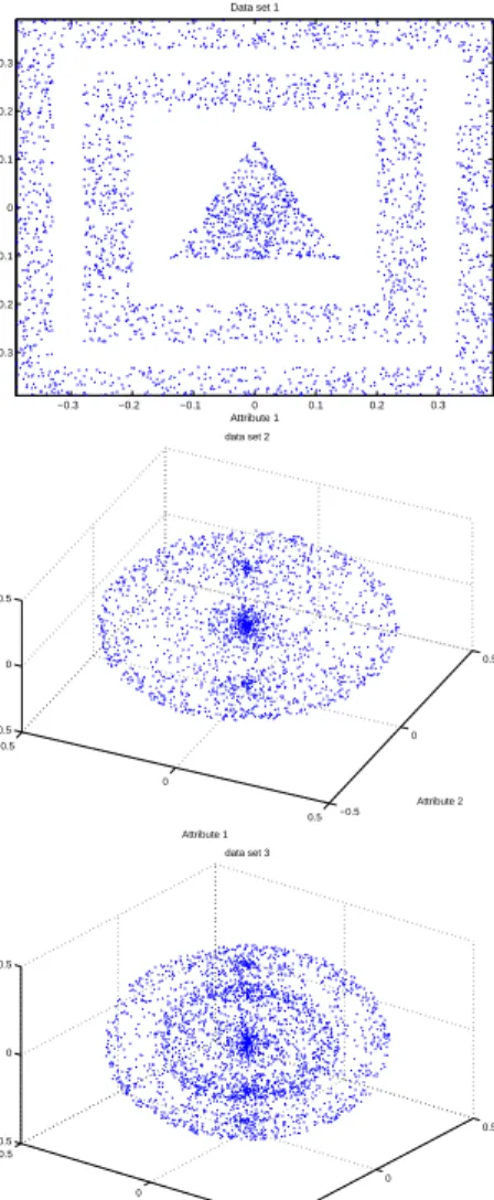
We have examined the ESOM on 3 synthetic data sets and 2 real-life data sets. Table 1 shows the properties of the five data sets. The first three synthetic data sets are interesting in both their special cluster shapes and locations as illus-trated in Fig.3. The conventional clustering algorithms such as K-means and expectation-maximization (EM) are unable to identify the clusters. The fourth data set, Mars, contains the temperatures taken from the Mars Pathfinder’s three sensors in different height. The fifth data set, Viking 2, contains the measurements of solar longitude, wind speed, pressure, and temperature taken from the Viking Lander 2. The Mars and Viking 2 data sets are downloaded from the web site ”The Live from Earth & Mars” of University of Washington
(http://www-k12.atmos.washington.edu/k12/resources/mars data-information/data.html). All data sets have been pre-processed by using the linear transformation
de-scribed in Eq.(2) in order to compare results fairly. The initial values of ², σ, andR are 0.5, 0.9 and 0.999 respectively. The values ofα andσ are decreased
by 0.998 per iteration. Except for the Mars data set, we have used a rectangu-lar grid with 20*20 neurons. As there are not many data items in Mars data sets, an output grid with 10 * 10 neurons is used. All experiments have been executed for 2000 iterations.
−0.3 −0.2 −0.1 0 0.1 0.2 0.3 −0.3 −0.2 −0.1 0 0.1 0.2 0.3 Attribute 1 Attribute 2 Data set 1 −0.5 0 0.5 −0.5 0 0.5 −0.5 0 0.5 Attribute 2 data set 2 Attribute 1 Attribute 3 −0.5 0 0.5 −0.5 0 0.5 −0.5 0 0.5 Attribute 2 data set 3 Attribute 1 Attribute 3
Fig. 3. Illustration of the 3 synthetic data sets, Data Set 1 (Upper), Data Set 2 (Middle) and Data Set 3 (Lower)
Researchers have introduced several measures to evaluate the quality of a mapping [1, 17]. In this paper, we employ the topological error ET used in
[5, 15] to evaluate the mapping obtained by our ESOM. ET is defined as
neurons are not adjacent on the grid. On the other hand, since the number of data items is normally larger than the number of output neurons, the weight vectors in the trained SOM become representatives of the original data set. The quantization error evaluates how well the weight vectors represent the data set [5, 16]. It is specified as follows:
EQ = 1 N N X k=1 k~xk(t)−w~mk(t)k (14)
where mk is the winner for the data vector ~xk(t). These two criteria usually
conflict in the SOM.
4.1 Results of 10 independent runs
We have performed 10 independent runs of both algorithms for the five data sets. The average topological errors, the average quantization errors and the average execution time are summarized in Tables 2, 3 and 4 respectively. Table 2
Average Topological Errors based on 10 independent runs.
Data Set Name ESOM SOM Improvement (%)
Data Set 1 0.24088 0.26039 7.49154 Data Set 2 0.30215 0.30555 1.11241 Data Set 3 0.33132 0.34763 4.69203
Mars 0.47059 0.53589 12.18534
Viking 2 0.79041 0.82103 3.72946
Table 3
Average Quantization Errors based on 10 independent runs.
Data Set Name ESOM SOM Improvement (%)
Data Set 1 0.01767 0.01800 1.80060 Data Set 2 0.04753 0.04832 1.64508 Data Set 3 0.05991 0.06042 0.83417 Mars 0.01308 0.01305 -0.22989 Viking 2 0.02370 0.02369 -0.04221 Table 4
Average Execution Times based on 10 independent runs.
Data Set Name ESOM SOM Difference (%)
Data Set 1 2371.6 2283.2 3.87176 Data Set 2 2068.9 2051.2 0.86291 Data Set 3 2904.7 2872.1 1.13506
Mars 32.3 31.7 1.85758
Viking 2 4844 4704 2.89017
sets are 0.01767, 0.04753 and 0.05991, which are little smaller than those of the SOM. The average topological errors of the ESOM are 0.24088, 0.30215, and 0.33132 respectively. They are 7.49152%, 1.11241% and 4.69203% smaller than those of SOM. In addition, the ESOM only needs little longer execution time as listed in Table 4. Therefore, for the synthetic data sets, the ESOM generates better mappings than the SOM in terms of both the topological and
the quantization errors with similar execution time.
For the first real-life data, the topological error of ESOM is 0.47059, which is 12.18534% shorter than the value of the SOM, 0.53589. On the other hand, the quantization error of ESOM is only 0.22989% larger than the one of the SOM. Similar comparison is found for the second real-life data set, where the ESOM makes 3.72946% improvement on the topological error and only 0.04221% loss on the quantization error. The gain on the topological error is very obvious in comparison with the loss on the quantization error. Therefore, using similar execution time, the ESOM can generate mappings with much better topological errors than the SOM. The ESOM has similiar quantization errors as SOM.
4.2 Typical results for the synthetic data sets
0 200 400 600 800 1000 1200 1400 1600 1800 2000 0.015 0.02 0.025 0.03 0.035 0.04 0.045 0.05 0.055
Quantization Error of Data Set 1
Number of Iterations Quantization Error SOM ESOM 0 200 400 600 800 1000 1200 1400 1600 1800 2000 0.1 0.2 0.3 0.4 0.5 0.6 0.7 0.8
Topological Error of Data Set 1
Number of Iterations
Topological Error
SOM ESOM
Fig. 4. The quantization error (Left) and the topological error (Right) during the learning of the ESOM and the SOM for the first data set.
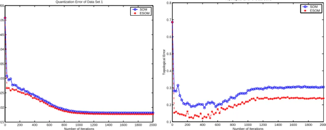
Fig.4 illustrates the quantization and the topological errors during a typi-cal run on the first data set of both algorithms. It is clearly seen that the quantization error decreases gradually as the learning process continues. The quantization error of the trained ESOM is 0.017 which is a bit smaller than
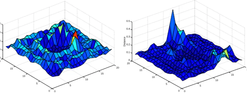
0 5 10 15 20 0 5 10 15 20 0 0.05 0.1 0.15 0.2 U−Matrix of ESOM Distance 0 5 10 15 20 0 5 10 15 20 0 0.1 0.2 0.3 0.4 0.5 U−Matrix of SOM Distance
Fig. 5. U-Matrix of the trained ESOM (Left) and the trained SOM (Right) for the first data set.
that of the trained SOM, 0.018. During learning, the decreasing, the increas-ing and the convergincreas-ing stages can be observed in the topological error curve. At the very beginning of the training process, the neuron’s weights are fairly dislike, while some of them even contain remnants of random initial values, thus higher topological errors are obtained. After executing several iterations, the topological error decreases dramatically. Because the learning rate ² and the neighborhood function are large, the neurons adjacent on the grid may move much closer to the input data item together. At this stage, the ESOM can learn the ordering topology of data items quickly. As shown in Fig.4, the topological error of the ESOM is much smaller than that of the SOM. The final topological errors of the ESOM and the SOM are 0.238 and 0.304 respec-tively, ESOM gains about 20% improvement. Thus, the ESOM can generate better topology preserving maps than the SOM.
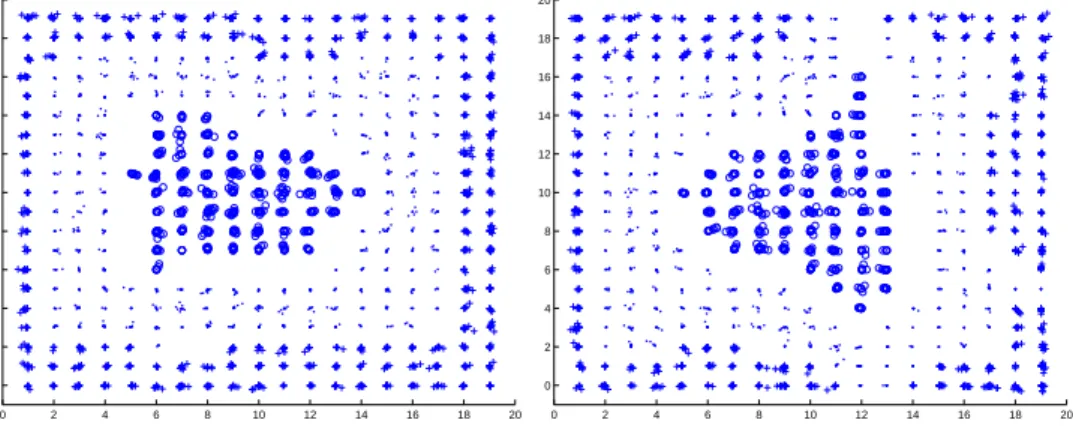
Fig.5 illustrates the trained ESOM and SOM for the first data set in the form of U-matrix. The x-axis and the y-axis of the U-matrix indicate a neuron’s position on the grid, and the z-axis is the average Euclidean distance of neurons from its adjacent ones [3]. A sequence of consecutive peaks can be regarded as a boundary among clusters, while the basins are regarded as clusters. There
0 2 4 6 8 10 12 14 16 18 20 0 2 4 6 8 10 12 14 16 18 20
Scatter Plot of ESOM
0 2 4 6 8 10 12 14 16 18 20 0 2 4 6 8 10 12 14 16 18 20
Scatter Plot of SOM
Fig. 6. Scatter plot the trained ESOM (Left) and the trained SOM (Right) for the first data set.
are clearly two sequences of peaks in the ESOM’s U-matrix, which indicate three clusters in the first data set. The layer structure in the data set is clearly illustrated. In contrast, The boundaries in the SOM’s U-matrix is not so clear because some high peaks blur the boundaries. The scatter plots shown in Fig.6 illustrate data clusters on the grid. In the scatter plot, each marker represents a mapping of a data item and the shape of the marker indicates its cluster label. The marker is placed on the winning neuron of the data item. To avoid overlapping, the marker has plotted with a small offset which is determined according to the data item’s Euclidean distance from the winning neurons. The ESOM maps data items in well-organized layers. We can easily find the three clusters in its scatter plot which is quite similar with the original data set as shown in Fig.3. However, the SOM cannot map the data items very well. The outer cluster in Fig.3 is even separated into three subclusters (indicated by ‘+’).
Fig.7 illustrates the scatter plots of a typical run of both algorithms for the second data set. The scatter plot of the ESOM clearly shows two clusters where one cluster surrounds the other as in the original data set depicted in
0 2 4 6 8 10 12 14 16 18 20 0 2 4 6 8 10 12 14 16 18 20
Scatter Plot of ESOM
0 2 4 6 8 10 12 14 16 18 20 0 2 4 6 8 10 12 14 16 18 20
Scatter Plot of SOM
Fig. 7. Scatter plot the trained ESOM (Left) and the trained SOM (Right) for the second data set.
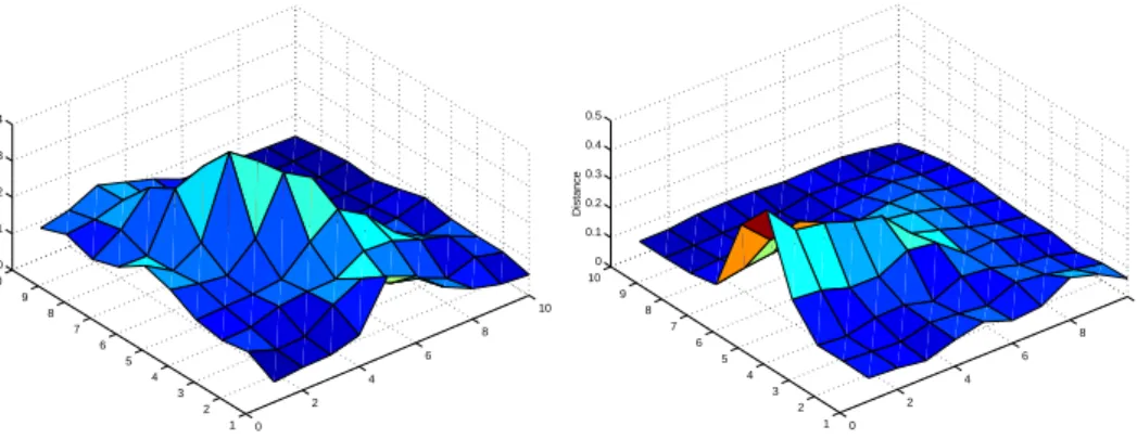
0 2 4 6 8 10 1 2 3 4 5 6 7 8 9 10 0 0.1 0.2 0.3 0.4 U−Matrix of ESOM Distance 0 2 4 6 8 10 1 2 3 4 5 6 7 8 9 10 0 0.1 0.2 0.3 0.4 0.5 U−Matrix of SOM Distance
Fig. 8. U-Matrices of the ESOM (Left) and the SOM (Right) for the Mars data set. Fig.3. In contrast, the SOM separates one of the clusters in the original data set into two clusters(represented by ‘.’).
4.3 Typical results for the real-life data sets
Fig.8 illustrates the U-matrices during a typical run on the Mars data set of both algorithms. By comparing all the data items and the weight values of all the neurons in the trained ESOM and SOM respectively, we have found that both of the algorithms are able to discover two clusters, but only ESOM can show the boundary clearly in the U-matrix.
From the above experimental and comparison results, we conclude that the ESOM can generate better topology preserving mappings than the SOM in terms of both the topological error and quantization error. The ESOM is more likely to identify the correct clusters from data sets than the SOM.
5 Conclusion
In this paper, we have proposed an Expanding Self-Organizing Map (ESOM) to detect and preserve better topology correspondence between the input data space and the output grid. During the learning process of our ESOM, the flexible neuron net is expanding and the neuron corresponding to a distant data item gets large expanding force. Besides the neighborhood relationship as in the SOM (Self-Organizing Map), the ESOM can detect and preserve a linear ordering relationship as confirmed by our theoretical analysis. Our experiment results have substantiated that, with similar execution time, the ESOM constructs better visualization results than the classic SOM, especially, in terms of the topological error. Furthermore, clustering results generated by the ESOM are more accurate than those obtained by the SOM on both the synthetic and the real-life data sets.
A rigorous theoretical analysis of the ESOM algorithm is subject to our future work, which heavily relies on the convergence analysis of SOM. We are also in-terested in applying the ESOM algorithm to large-scale and high-dimensional data sets.
6 Acknowledgement
This research was supported by RGC Earmarked Grant for Research CUHK 4212/01E of Hong Kong.
References
[1] H. U. Bauer, M. Herrmann, and T. Villmann. Neural maps and topo-graphic vector quantization. Neural Networks, 12:659–676, 1999.
[2] C. M. Bishop, M. Svensen, and C. K. I. Williams. Gtm: a principled al-ternative to the self-organizing map. InProceedings of ICANN’96, Inter-national Conference on Artificial Neural Networks, pages 165–170, 1996. [3] J.A.F. Costa and M.L. de Andrade Netto. A new tree-structured self-organizing map for data analysis. In Proceedings of International Joint Conference on Neural Networks, volume 3, pages 1931–1936, 2001. [4] Huidong Jin, Kwong-Sak Leung, and Man-Leung Wong. An integrated
self-organizing map for the traveling salesman problem. In Nikos Mas-torakis, editor,Advances in Neural Networks and Applications, pages 235– 240, World Scientific and Engineering Society Press, Feb. 2001.
[5] J. S. Kirk and J. M. Zurada. A two-stage algorithm for improved topog-raphy preservation in self-organizing maps. In 2000 IEEE International Conference on Systems, Man, and Cybernetics, volume 4, pages 2527– 2532. IEEE Service Center, 2000.
[6] Teuvo Kohonen. Self-Organizing Maps. Springer-Verlag, New York, 1997. [7] Teuvo Kohonen, Samuel Kaski, Krista Lagus, Jarkko SalojAvi, Vesa Paatero, and Antti Saarela. Organization of a massive document col-lection. IEEE Transactions on Neural Networks, Special Issue on Neural
Networks for Data Mining and Knowledge Discovery, 11(3):574–585, May 2000.
[8] R.D. Lawrence, G.S. Almasi, and H.E. Rushmeier. A scalable parallel algorithm for self-organizing maps with applications to sparse data mining problems. Data Mining and Knowledge Discovery, 3:171–195, 1999. [9] Siming Lin and Jennie Si. Weight-value convergence of the SOM
algo-rithm for discrete input. Neural Computation, 10(4):807–814, 1998. [10] Z. Meng and Y.-H. Pao. Visualization and self-organization of
multidi-mensional data through equalized orthogonal mapping. IEEE Transac-tions on Neural Networks, 11(4):1031–1038, July 2000.
[11] U. Seiffert and B. Michaelis. Adaptive three-dimensional self-organizing map with a two-dimensional input layer. In Intelligent Information Sys-tems, 1996., Australian and New Zealand Conference on , 1996, pages 258 –263, 1996.
[12] Mu-Chun Su and Hsiao-Te Chang. A new model of self-organizing neural networks and its application in data projection. IEEE Transactions on Neural Networks, 12(1):153 –158, Jan. 2001.
[13] A. Tenhagen, U. Sprekelmeyer, and W.-M. Lippe. On the combination of fuzzy logic and kohonen nets. InIFSA World Congress and 20th NAFIPS International Conference, 2001. Joint 9th, pages 2144 –2149, 2001. [14] Juha Vesanto. SOM-based data visualization methods. Intelligent Data
Analysis, 3:111–26, 1999.
[15] Juha Vesanto. Neural network tool for data mining: SOM toolbox. In Pro-ceedings of Symposium on Tool Environments and Development Methods for Intelligent Systems (TOOLMET2000), pages 184–196, Oulu, Finland, 2000.
IEEE Transactions on Neural Networks, 11(3):586–600, May 2000. [17] Thomas Villmann, Ralf Der, Michael Herrmann, and Thomas M.
Mar-tinetz. Topology preservation in self-organizing feature maps: exact defini-tion and measurement. IEEE Transactions on Neural Networks, 8(2):256 –266, March 1997.
[18] Hujun Yin and Nigel M. Allinson. Self-organizing mixture networks for probability density estimation. IEEE Transactions on Neural Networks, 12:405 –411, March 2001.