Surface Reconstruction from Noisy Point Clouds

M. Desbrun, H. Pottmann (Editors)

Surface Reconstruction from Noisy Point Clouds

University of California at Davis

IMPA - Instituto Nacional de Matematica Pura e Aplicada

Abstract

We show that a simple modification of the power crust algorithm for surface reconstruction produces correct outputs in presence of noise. This is proved using a fairly realistic noise model. Our theoretical results are related to the problem of computing a stable subset of the medial axis. We demostrate the effectiveness of our algorithm with a number of experimental results.

Categories and Subject Descriptors(according to ACM CCS): I.3.3 [Computer Graphics]: Surface Reconstruction, Medial Axis, Noisy samples

1. Introduction

Surface reconstruction is an important problem in geometric modeling. It has received a lot of attention in the computer graphics community in recent years because of the develop-ment of laser scanner technology and its wide applications in areas such as reverse engineering, product design, medi-cal appliance design and archeology, among others.

Different approaches have been taken to the problem, in-cluding the work of Hoppe, DeRose et al which popular-ized laser range scanning as a graphics tool [HDD∗_{92], the} rolling ball technique of Bernardini et al [BMR∗_{99], the} vol-umetric approach of Curless et al [CL96] used in the Digital Michelangelo project [LPC∗_{00], and the radial basis} func-tion method of Beatson et al. [CBC∗_01].

The algorithms [ABK98,ACDL00,BC02,ACK01a] uses the Voronoi diagram of the input set of point samples to produce a polyhedral output surface. A fair amount of the-ory was developed along with these algorithms, which was used to provide guarantees on the quality of the output under the assumption that the input sampling is everywhere suffi-ciently dense. The theory relates surface reconstruction to the problem of medial axis estimation in interesting ways, and shows that the Voronoi diagram and Delaunay triangu-lation of a point set sampled from a two-dimensional surface have various special properties. Some strengths of the sam-pling model used are that the required samsam-pling density can vary over the surface with the local level of detail, and that

over-sampling, in arbitrary ways, is allowed. One drawback is that it assumes that the sample is free of noise.

When noise is considered as well, the quality of the out-put is related to both the density and to the noise level of the sample. A small number of recent results have begun to explore the space of what it is possible to prove under vari-ous noisy sampling assumptions. Dey and Goswami [DG04] proposed an algorithm for which they could provide many of the usual theoretical guarantees, using a model in which both the sampling density and the noise level can vary with the local level of detail, but which gives up the arbitrary over-sampling property. A real noisy input, however, might well have arbitrary over-sampling but the sampling density and noise level usually varies unpredictably, independent of the local level of detail.

In this paper, we show that similar results can be achieved given bounds on the minimum sampling density and maxi-mum noise level, but allowing arbitrary over-sampling.

Related Work

Most of the algorithms using the Voronoi diagram and De-launay triangulation of the samples, for which a variety of theoretical guarantees can be provided, require the input to be noise-free [AB99,ACDL00,ACK01b,BC02]. In prac-tice some of these algorithms are more sensitive to noise than others. The recent algorithm of Dey and Goswami [DG04] extends much of the theory developed in the noise-free case

a) b)

c) d)

f)

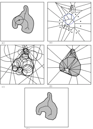
Figure 1:A two dimensional example of the power crust al-gorithm. a) An object and its medial axis. b) The voronoi di-agram and its poles, the blue points corresponding to poles and the circles corresponding to polar balls. c) The set of inner and outer polar balls. d) The power diagram of the set of polar balls. The algorithms labels the cells of this power diagram inner or outer. e) The set of faces in the power dia-gram which separate inner from outer cells.

to inputs with noise. We do the same with a less restrictive sampling model, as described in more detail in Section2.2.

Both our algorithm and that of Dey and Goswami are ex-tensions of thepower crustalgorithm proposed by Amenta, Choi and Kolluri [ACK01b]. This algorithm is illustrated in Figure1. Given an input sample Pof points on a sur-faceS, it selects from the Voronoi diagram ofPa setV of Voronoi vertices, thepoles, which approximate the medial axis transform ofS. It then uses thepower diagram(a kind of weighted Voronoi diagram) of the set of Delauanay balls centered atV (thepolar balls) to recover a polyhedral sur-face representation.

Voronoi-based surface reconstruction techniques in gen-eral are closely related to Voronoi-based algorithms for me-dial axis estimation (in fact the power crust code is probably more often used for the latter problem). Yet another noisy sampling model was used by Chazal and Lieutier [CL05] in a recent paper on medial axis estimation: their sampling re-quirement is simply that the Hausdorff distance between the

point sample and the surface itself is bounded by some con-stantr. Notice that this allows for arbitrary over-sampling, but does not allow the sampling density to vary over the sur-face according to the local level of detail. Chazal and Lieu-tier proved, drawing on more general results, that a subset of the Voronoi diagram ofPapproaches a subset of the medial axis ofSasr→0, and that both converge to the entire me-dial axis. It is tempting to apply Chazal and Lieutier’s result directly to the surface reconstruction problem, by using the power crust approach to produce a polyhedral surface from their approximate medial axis. But this is not as straightfor-ward as it might seem: their medial axis estimation includes Voronoi edges and two-faces as well as vertices, while the analysis of the power crust relays on having an approxima-tion of the medial axis by Voronoi vertices. Also, the subset of the medial axis approximated by Chazal and Lieuter is not guaranteed to be homotopy equivalent to the complete me-dial axis, or to the object, since the sampling is not required to be dense enough to capture the smallest topological fea-ture.

Recently similar techniques have been used to analyze a particular smooth surface determined by a noisy sets of samples [Kol05], a variant of the MLS surface definition of Levin [Lev03]. In this case arbitrary over-sampling seems to be ruled out, since the surface locally averages the input samples and malicious over-sampling could influence the lo-cal averages. There is also a recent algorithm for curve re-construction from a noisy sample [CFG∗_{03] with theoretical} guarantees, for which the sampling model has the interest-ing property that the quality of the output improves with in-creased sampling density, even when the noise level remains constant. The sampling model used is not particularly realis-tic, but the property seems quite relevant to practice.

2. Geometric Definitions and Sampling Assumptions 2.1. Defnitions and Notation

We will use the following notation. For any setX⊂R3,Xo,

Xcand∂Xdenote respectively the interior ofX, the comple-ment ofXand the boundary ofX. Given a pointxand a set

Y we denote byd(x,Y) =infy∈Yd(x,y). Given any two set XandY we denote by ˜dH(X,Y) =sup_x∈Xd(x,Y)the one-sided Hausdorff distance fromX toY and bydH(X,Y) =

max{dH˜ (X,Y),dH˜ (Y,X)_}the Hausdorff distance betweenX

andY. We denote byBc,ρa ball with centercand radiusρ. We will consider two-dimensional, compact, andC2 man-ifolds without boundary, and we will call such a manifold a

smooth surface. LetSbe a smooth surface. We will assume thatSis contained in an open, bounded domainΩ(eg, a big open ball). The surfaceSdividesΩ into two open solids, the inside (inner region) and the outside (outer region) ofS, which are disconnected.

Themedial axis Mof a surfaceSis the closure of the set of points inΩthat have at least two distinct nearest points

onS. Note that the setMis divided into two parts, the inner and outer medial axis, belonging to the inner or outer region of the surfaceS, respectively. The ballBm,ρm centered at a medial axis pointmwith radiusρm=d(m,S)will be called

amedial ball. It is easy to see that a medial ball is maximal in the sense that there is no ballBwith Bo∩S=_∅which containsBm,ρm.

The medial axisMis a bounded set, since in our definition it is contained in the bounded domainΩ. So there exits an upper bound∆0for the radius of the medial balls.

2.2. Sampling and Noise Models

There are at least two good approaches to defining sampling and noise models. First, we can begin with a model which we believe roughly describes the characteristics of reason-able input data sets, and then show that our algorithm works correctly on data that fits the model. The second approach would be to begin with the algorithm, and describe the data sets for which the algorithm is correct as broadly as possi-ble, and then argue that this broad class of possible inputs includes reasonable input data sets (possibly among others). This is the approach taken in the analysis of many of the Voronoi-based surface reconstruction algorithms, as follows. For a pointx∈S, we define lfs(x) =d(x,M). This lfs

func-tion is used to determine the required sampling density; it is small in regions of high curvature or where two patches of surface pass close together, and larger away from such re-gions of fine detail.

A finite set of pointsPis ar-sampleof the surfaceSifP⊂ Sand if for anyx∈Sthere is a point p∈Pwithd(x,p)_≤

rlfs(x).

The points of a noisy samplePforSlie near but not on the surface. Let ˜Pbe the projection of the setPontoS, taking each pointp∈Pto its closest point ˜p∈S. Dey and Goswami in [DG04] introduced the definition of anoisy(k,r)-sample: Definition 1Noisy(k,r)-sample. A finite set of pointsPis a noisy(k,r)-sample if the following conditions hold:

1. ˜Pis ar-sample ofS.

2. For anyp∈P;d(p,p˜)_≤c1rlfs(p˜)for some constantc1. 3. For any p∈P;d(p,q)_≥c2rlfs(p˜), whereqis thekth

nearest sample top, for some constantc2.

Here the first condition requires the sample to be dense enough, the second condition bounds the noise level, and the third condition requires that the sample is nowhere too dense (by requiring thekthnearest sample to be far enough away). The third condition does not seem strictly necessary, and one of the contributions of this paper is to show that indeed it is not, at least for many of the geometric results used in the analysis. We will adopt a definition which we call anoisy r-sample, essentially only using conditions i) and ii):

Definition 2Noisy r-sample. A finite set of pointsPis a noisyr-sample if the following two conditions hold: 1. ˜Pis ar-sample ofS.

2. For anyp∈P,d(p,p˜)_≤k1rlfs(p˜), for some constantk1.

We define lfs(S) =minx∈Slfs(x) for the surface as a

whole. Assuming S is C2 we have lfs(S)>0 [APR02]. We also define the maximum local feature size ∆1 =

maxx∈Slfs(x)and we have∆1≤∆0 (recall that∆0 is the radius of the largest medial ball).

3. Geometric constructions and the algorithm

To avoid to dealing with infinite Voronoi cells, we add to the sample setPa setZ of eight points, the vertices of a large box containingΩ.

The concept ofpoles was defined by Amenta and Bern [ACK01b] as follows:

Definition 3The poles pi, po of a sample p∈P, are the two vertices of its Voronoi cell farthest fromp, one on either side of the surface. The Voronoi ballsBpi,ρpi,Bpo,ρpo are the polar balls with radiiρpi =d(pi,p)andρpo=d(po,p) re-spectively.

Notice that given a noisy sample set not all Voronoi cells are long and skinny, as they are in the noise-free case.

A polar ballBv,ρvis classified as an inner (outer) polar ball if its center is inside the inner (outer) region ofR3\S. We denote byPIandPOthe set of all inner and outer polar balls,

respectively.

Algorithm

Our algorithm consists of a very simple modification to the power crust algorithm: we discard any poles such that the radius of the associated polar ball is smaller thanlfs(S)

c where c>1 is a constant.

This can be summarized as follows. Algorithm 3.1Power Crust

1. Compute the Delaunay Diagram ofP∪Z.

2. Determine the setPof polar balls.

3. Delete fromPany ball of radius<lfs(_cS), producingP0_. 4. Compute the power diagram ofP0

5. Label the balls inP0as outer balls or inner balls, resulting in the setsBOandBI.

6. Determine the faces in Pow(BO∪_BI)separating inner from

outer cells.

We discuss the labeling in step five in the AppendixA. It is done using exactly the same method as in the original power crust algorithms, but to show that it remains correct in the noisy case we need to prove a few more lemmas.

Analysis Overview

Most of our paper is concerned with the proof that this simple modification produces an output polyhedral surface which is correct, topologically and geometrically, given a noisyr-sample. Some of the lemmas are true for constant

rindependent ofS, The lemmas6-9and Theorems1and2 requiresr=O(lfs_∆(₁S)).

We prove that a subset of the medial axis can be well ap-proximated by the set of poles, this is stated in Lemma6. As a consequence of this fact we prove in Lemma8that the boundary of the union of the set of big inner (outer) polar balls (see Equations1and2) is close to the sampled sur-face, in the sense of Hausdorff distance. We use this fact in turn to show that the Hausdorff distance between the power crust and the sampled surface isO(√4_{r) (Theorem1) and} that the power crust is homeomorphic to the original surface

S(Theorem2).

4. Union of polar balls

Given a constantc>1 we define the following two polar

ball subsets: BI = {Bc,ρc∈PI : ρc≥ lfs(S) c } (1) BO = {Bc,ρc∈PO : ρc≥ lfs(S) c } (2)

The setsBIandBOare the sets of balls retained in our mod-ified power crust algorithm. Their respective boundary sets are:SI=∂(S

B∈BIB)andSO=∂( S

B∈BOB). Our goal will be to prove that the boundary sets SI and SOare close to the surfaceS. Moreover, we will prove that a subset of the two-dimensional faces of the power diagram ofBI∪BOis

homeomorphic to the surfaceS.

Our proofs will also use another pair of subsets of the po-lar balls. We denote byB0_IandB0_Othe set of inner and outer polar balls where each ball contains a medial axis point. That is,

B0I = {Bc,ρc∈PI : Bc,ρc∩M6=∅ } (3) B0O = {Bc,ρc∈PO : Bc,ρc∩M6=∅ } (4) The following lemma proves thatB0_{I ⊂}BIandB0_O⊂BO

respectively.

Lemma 1B0I⊂BIandB0_O⊂BO, forc>2 andr< c_k−2_1c.

Proof Take a ball Bx,ρ∈B0_I (Bx,ρ_∈BO). There exists a

sample pon∂Bx,ρand there exists an inner (outer) medial axis pointminsideBx,ρ. Then we have thatd(p˜,p) +2ρ≥ d(p˜,p) +d(p,m)≥d(p˜,m)≥lfs(p˜), and consequentlyρ≥

lfs(p˜)−d(p,p˜ )

2 ≥1−2k1·r·lfs(p˜). Takingr≤ ck−21c we get that

ρ≥lfs(p˜)/c≥lfs(S)/c.

The next lemma is a consequence of the sampling require-ments and will be used for later proofs.

Lemma 2Given Pa noisyr-sample ofS, letDbe a ball withDo∩P=∅andD∩S6=∅, letxbe a point inD∩S. If

B(x,ρx)_⊂Dthenρx≤r(1+2k1)lfs(x).

Proof By sampling condition 1 of Definition2.there exists a sampleqsuch thatd(x,q˜)_≤rlfs(x). Using the fact that lfs is a one-Lipschitz function we have that lfs(q˜)_≤d(q˜,x) +

lfs(x)_≤rlfs(x) +lfs(x) = (1+r)lfs(x).

By the sampling condition 2 and the previous equation we getd(x,q)≤d(x,q˜) +d(q˜,q)≤rlfs(x) +k₁rlfs(q˜)≤(r+

2k1r)lfs(x). Since

o

D∩P=_∅one deduces thatB(xo,ρx)_∩P=

∅, henceρx≤d(x,q)≤r(1+2k1)lfs(x).

Also we have the following lemma from Amenta and Bern [AB99] which estimates the angle between the normals to the surface at two close points.

Lemma 3For any two points pandqonSwithd(p,q)_≤

rmin{lfs(p),lfs(q)_}, for anyr≤ 13, the angle between the normals toSatpandqis at most r

1−3r.

A central idea in Voronoi-based surface reconstruction is that the Voronoi cells of a dense enough noise-free sam-ple are long, skinny and perpendicular to the surface. This is not true for all Voronoi cells when there is noise, but the following lemma shows that it is true for large enough Voronoi cells. Specifically, given a sample point pand a pointx∈Vor(p)we bound the angle between the vectorxp~

and the surface normal~np˜ at the projection of the sample

pontoS. The lemma states that whenxis far away fromp, then this angle has to be small. In the noise-free case, “small" meantO(r); here we achieve a bound of onlyO(√r). Lemma 4Let p∈Pbe a sample such that there exists a pointxon the inner (outer) region of the Voronoi cell ofp

with distanceρxbetweenxand psatisfying the inequality

ρx≥lfsc(1p˜)for some constantc1. Then the angle between the vectorxp~ and the oriented outward (inward) surface normal

~np˜isO(√r).

ProofDenote byBm,ρm the outer (inner) medial ball tangent to the surfaceSat ˜p. LetBx,ρxbe the ball centered atxwith radiusρx=d(x,p). Sincexis in the Voronoi cell of pwe

haveBx,o ρx∩P=∅.

The angle between the vectors xp~ and ~np˜ is the sum

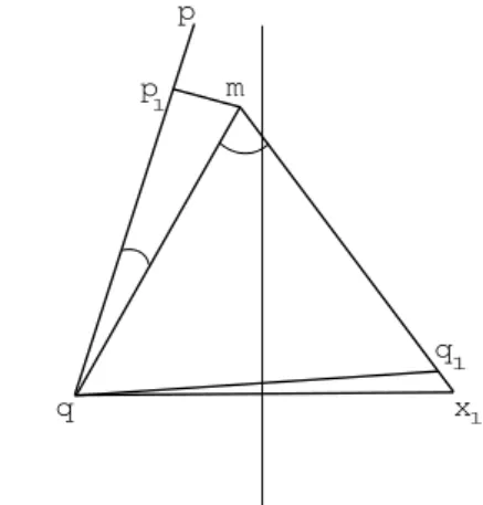
∠(t,x,p) +∠(t,m,p), where the segmentptis

perpendicu-lar toxm, see figure2. Our aim will be to find upper bounds for the angles∠(t,x,p)and∠(t,m,p), respectively. Since

d(x,t)<d(x,p) =ρx, we have thatt∈Bx,ρx, and the fol-lowing two situations are possible: eithert∈Bm,ρm∩Bx,ρx ort_∈Bc

m,ρm∩Bx,ρx.

First case:t∈Bm,ρm∩Bx,ρx, see figure2left. Sincet∈Bm,ρm we have thattis on the outer (inner) region ofΩ\Sand the raylxcontainingxandtintersects the surface at the pointts

n

Figure 2:Left: Illustration of Lemma 4, a fundamental result describing the shape of the Voronoi cells. When there exists a point x in Vor(p)such that d(x,p)≥ lfsc(p˜) then the angle between the segmentxp and the normal~ ~np˜ is a O(√r). Center: Figures

used in the proof of Lemma 4. t∈Bm,ρm∩Bx,ρx. Right t∈Bcm,ρm∩Bx,ρx

segment[x,t]_⊂Bx,ρx. Moreover, the raylxintersects∂Bx,ρx at the pointbx, see figure2. Using thatts∈Bx,ρxwe have, for small enoughr, the following inequality that will be useful later:

lfs(ts) _≤ d(ts,p˜) +lfs(p˜)_≤ρx+d(x,p) +d(p,p˜) +lfs(p˜)

≤ 2ρx+ (1+r·k1)lfs(p˜)≤(2+2c1)ρx=kcρx(5) Because the pointstsandbxare inside the ballBx,ρxwe have thatBts,d(ts,bx)⊂Bx,ρx. SinceBx,ρx is empty of samples (be-causeρxis the distance ofxto its closest point inP), we have thatBt_s,d(ts,bx) is also empty of samples. Consequently, by Lemma2, we obtaind(ts,bx)_≤O(r)lfs(ts). From this last equation together with equation5and the fact thatt∈[bx,ts]

we obtain the following two inequalities:

d(t,bx)_≤d(ts,bx)_≤O(r)lfs(ts)_≤O(r)ρx (6) d(t,ts)_≤d(ts,bx)_≤O(r)lfs(ts)_≤O(r)ρx (7) Consequently, by6we haved(t,x) =ρx₋d(t,bx)_≥(1− O(r))ρx, hence d(p,t) = q d(p,x)2₋d(x,t)2=O(√r)ρx (8) so, the angle∠(t,x,p)is bounded by

∠(t,x,p) =arcsin _d (p,t) ρx =O(√r) (9)

On the other hand, sincet∈Bm,ρm, we have that lfs(ts)<

d(ts,t) +d(t,m)_≤O(r)lfs(ts) +ρm, thus obtaining lfs(ts)<

ρm

1−O(r). Because the pointsm,t,tsare collinear,t∈Bm,ρm

andts_∈/Bm,ρo m. So we obtain the following lower bound for the distance betweentandm:

d(t,m)≥ρm−d(t,ts)≥ρm−O(r)lfs(ts)>(1−O(r))ρm

.

Since lfs(p˜)<ρm, and using the sampling conditions, we get thatd(p,m)<d(m,p˜) +d(p˜,p)_≤(1+O(r))ρm, conse-quently

d(p,t) = q

d(p,m)2₋d(t,m)2=O(√r)ρm (10) We have thatρm=d(m,p˜)_≤d(m,p) +d(p,p˜), so using that lfs(p˜)<ρm we haved(m,p)≥ρm−d(p˜,p)≥(1− O(r))ρm. From this equation and Equation10we can bound the angle∠(t,m,p)as follows:

∠(t,m,p) =arcsin _d (p,t) d(m,p) =O(√r) (11)

Therefore, from 9 and 11 we have that our target angle

∠(t,x,p) +∠(t,m,p)isO(√r).

Second case: t∈Bcm∩Bx,ρx (Note that this case implies that Bm,ρm∩Bx,ρx =∅). Since t ∈/ Bm,ρm and d(p,m) ≥

d(t,m) we obtain that p_∈/Bm,ρm, consequently we have thatd(t,∂Bm,ρ_m)_≤d(p,∂Bm,ρ_m) =d(p,p˜)_≤O(r)lfs(p˜), see Figure2right. From this inequality and using the fact that

t∈Bx,ρxwe get

d(t,x)≥ρx−d(t,∂Bm,ρm)≥ρx−O(r)lfs(p˜) (12) Since lfs(p˜)≤d(p˜,p) +d(p,x)≤O(r)lfs(p˜) +ρxwe get

lfs(p˜)_≤ ρx

1−O(r). Consequently Equation12can be

O(r))ρx. We deduce the following upper bound for the dis-tance betweenpandt

d(p,t) = q

d(p,x)2−d(t,x)2=O(√r)ρx

Therefore, we have ∠(t,x,p) = arcsind_d(_(x,pp,t)₎ ≤

arcsinO(√r)ρx

ρx

=O(√r).

On the other hand, since t _∈/ Bm,ρm we get d(t,m) >

ρm.d(p,m)_≤d(p,p˜) +d(p˜,m)_≤O(r)lfs(p˜) +ρm= (1+

O(r))ρm, and hence

d(p,t) = q

d(p,m)2−d(t,m)2=O(√r)ρm

and the angle ∠(t,m,p) = arcsind(p,t)

d(p,m) ≤ arcsinO(√r)ρm ρm

= O(√r). Thus we conclude that the

angle∠(t,x,p) +∠(t,m,p)isO(√r).

As a consequence of this lemma, we have that the inner and outer parts of the medial axisMare inside the setsS

B∈BI o B andS B∈BO o

Brespectively, this is stated in the next lemma. Lemma 5Given an inner (outer) medial axis pointm, then there exists an inner (outer) polar ballB∈BI(B∈BO)such

thatm∈Bo.

Proof There exists a sample p such that m is inside its Voronoi cell. Denote byqthe inner (outer) pole ofp. Then by the definition of local feature size we have d(m,p˜)_≥

lfs(p˜). By the triangle inequality we have d(m,p) +

d(p,p˜)_≥d(m,p˜), so we haved(m,p)_≥d(m,p˜)₋d(p,p˜)_≥

lfs(p˜)−r k₁lfs(p˜). Taking r ≤ ₂1k1 we get d(m,p) ≥ lfs(p˜)

2 . This fact along with Lemma 4implies that the an-gle ∠(mp~ ,~np˜) =O(√r), using the same argument. Since

d(q,p)_≥d(m,p)we obtain∠(~qp,~np˜) =O(√r). Hence we obtain∠(qp~ , ~mp) =O(√r).

We take r small enough such that ∠(qp~ , ~mp)≤ π₄. Since

d(m,p)_≤d(q,p) we find that mis inside the interior of the inner (outer) polar ball Bq,d(q,p). Hence, we have that

Bq,d(q.p)∈B0I (Bq,d(q,p)∈B0O). By Lemma1, B0I ⊂BI

(B0O⊂BO), completing the proof.

From now on assure thatr=O(lfs(S)/∆₁). We will show that the medial axis pointsmwith angle∠qmx1sufficiently large are well approximated by poles. The pointqis the clos-est sample tomandx1 is the closest sample of the closest surface point tom.

Lemma 6Letmbe a inner (outer) medial axis point such that

m∈Vor(q)for some sampleqand letpbe the inner (outer) pole of Vor(q). Let ˜x∈Sbe the closest point tomonSandx1 the closest sample to ˜x. Then we have_|d(m,x₁)₋d(m,q)_{| ≤}

O(r)and if the angle∠x1mq>√r, thend(m,p) =O(√r) and|d(m,x˜)−d(p,q)| ≤O(√r) q m x p q₁ 1 p 1

Figure 3:The medial axis point m∈Vor(q)is close to the pole p of Vor(q)when angle∠qmx1>√r

ProofFirst we proof that the distancesd(q,m)andd(m,x1) are close. Let ˜qbe the projection of the sampleqontoS, since ˜xis the closest sample tomthen we have thatd(m,q˜)_≥

d(m,x˜). Using thatd(m,q˜)≤d(m,q) +d(q,q˜)we have that

d(m,q)_≥d(m,x˜)₋O(r)lfs(q˜)_≥d(m,x˜)₋O(r)∆₁. Rea-soning in a similar way we have thatd(m,p)≤d(m,x1)

wherex1is the closest sample of ˜x, we have using the trian-gular inequalityd(m,p)_≤d(m,x1)≤d(m,x˜) +d(x˜,x1) =

d(m,x˜) +O(r)lfs(x˜)_≥d(m,x˜) +O(r)∆₁we get that:

|d(m,q)₋d(m,x˜)_{| ≤}O(r∆₁) (13) Using that|d(m,x˜)−d(m,x₁)| ≤O(r∆₁)together with

equa-tion13we get that

|d(m,q)₋d(m,x1)| ≤O(r∆1) (14) Sinced(m,q)≤d(m,x1)then there exists a pointq1in the segmentmx1such thatd(m,q1) =d(m,q), see figure3. Us-ing14we have thatd(q1,x1)≤O(r∆1).

Our goal is to bound the distance betweenpandm, in that direction we will prove that the distanced(p,p1) =d(p,q)−

d(m,q)andd(m,q₁)are small, so we will start by bounding

d(p,q).

The triangle qmq1 is isosceles we have that d(q,q1) =

2sin(∠qmq1/2)d(m,q) from this we get that d(q,x1) ≤

d(q,q1) +d(q1,x1) ≤ 2sin(∠qmq1/2)d(q,m) +O(r∆1).

Using this last equation we can bound the angle

∠q1qx1 ≤ arcsin(dd((qq,q1,x11))) ≤ arcsin(

O(r∆1)

2 sin(O(√r)d(m,q)) ≤

arcsin( O(r∆1)

2 sin(O(√r)lfs(S)) = O(√r∆1/lfs(S)). The an-gle ∠mqq1 satisfies that ∠mqq1 = π/2−∠qmq1/2. By the lemma 4 we can deduce that angle

∠pqm = O(√r). Combining all this angle we derive

that ∠pqx1 =π/2−∠qmq1/2+∠pqm+∠q1qx1. Using thatd(p,q)≤d(p,x1)we derive an upper bound ford(p,q)

d(p,q) _≤ d(q,x1)/2 sin(π/2−∠pqx1) = d(q,x1)/2 sin(∠qmq1/2−∠pqm−∠q1qx) ≤ _cos( d(m,q) ∠pqm+∠q1qx) + O(r∆1) sin(∠qmq1/2)cos(∠pqm+∠q1qx) = d(m,q) cos(O(√r∆₁/lfs(S))) + O( √_r∆ 1) cos(O(√r∆1/lfs(S))) (15)

Recall that maxs∈Slhf(s) =∆1<∆0, where∆0is the maxi-mum of the radius of the medial balls. From equation15and taking the constantrsuch that cos(O(√r∆1/lfs(S)))≥1/2

which implies thatr=O(lfs(S)/∆₁)we have that

d(p,p1) = d(p,q)−d(m,q) ≤ _cos(O(√d(_r∆m,q) 1/lfs(S))) + O( √_r∆ 1) cos(O(√r∆₁/lfs(S)))−d(m,q) = 1−cos(O( √_r∆ 1/lfs(S)) cos(O(√r∆₁/lfs(S))) d(m,q) +O( √_r∆ 1) = O(√r∆₁(1+∆₀/lfs(S))) (16)

On the other hand using13we have thatd(m,q)≤d(m,x˜) +

O(r∆₁) =∆₁+O(r∆₁), therefore we have that

d(m,p1) = 2sin(∠pqm/2)d(m,q)

≤ 2sin(O(√r))d(m,q) =O(√r∆₀) (17) Combining equations17,16we get that

d(m,p) ≤ d(m,p₁) +d(p₁,p)

≤ O(√r∆0) +O(√r∆1(1+∆0/lfs(S)))

= O(√r∆0(2+∆0/lfs(S))). (18)

Finally, using that |d(m,q)₋d(q,p)_{| ≤}d(p,p1) and the equation 13 we have that |d(m,x˜)−d(p,q)| ≤O(√r∆₁)

Using this fact, lemma6, one can derives that the bound-ariesSI andSOof the union of ballsS

B∈BIBand S

B∈BOB are close to the surfaceS. This is stated in lemma8, to prove this lemma a technical lemma7is first introduced.

Lemma 7LetBc1,ρ1 andBc2,ρ2 be two balls withBc1,ρ1∩

Bc2,ρ26=∅andBc2,ρ26⊂Bc1,ρ1. Letε<ρi,i=1,2 be such that

d(c1,c2)≤εand|ρ1−ρ2| ≤ε. Letx2be a point on∂Bc2,ρ2\

Bc1,ρ1and{x1}= [c2,x2]∩∂Bc1,ρ1. Thend(x1,x2)≤2ε.

ProofWe haved(x1,x2) =ρ2−d(c2,x1). By the triangular inequality we haved(c2,x1)≥d(c1,x1)−d(c2,c1) =ρ1−

d(c2,c1). From these two inequalities we obtaind(x1,x2)≤

ρ2−ρ1+d(c2,c1)≤ |ρ2−ρ1|+d(c2,c1)≤2ε Lemma 8dH(SI,S)≤O(√4_{r)anddH(SO,S)≤O(}√4_r).

ProofWe show thatdH(SI,S)≤O(√4_{r); the argument forSO} is identical. We begin by showing that ˜dH(SI,S)_≤O(√4_r). Consider any pointx∈SI. First assume thatxis on the out-side ofS. LetBc,ρc be a polar ball inBIsuch thatx∈∂Bc,ρc. Then the segment[c,x]from the center of the polar ball to

xintersectsSin a points. Since the ballBs,d(s,x) is inside

the polar ballBc,ρ, Lemma2implies thatd(x,S)_≤d(x,s) =

O(r)and we are done.

So let us assume thatx∈SI is in the inner region ofS. Let ˜

x∈Sbe the closest point toxonS, and letmx˜be the center of the inner medial axis ballBmx˜,ρx˜ tangent toSat ˜x. Then we have thatxis inside the segment[x˜,mx˜]; otherwise the ballBx,d(x,x˜)with

o

Bx,d(x,x˜)∩S=∅containsBmx˜,ρx˜which is a contradiction due to the ballBmx˜,ρx˜ is maximal.

The medial axis point mx˜ belongs to the Voronoi cell of some sample point q, let p and Bp,ρp be the in-ner pole of q and its polar ball respectively. The first part of lemma 6 states that the distances d(mx˜,x1) and

d(mx˜,q) where x1 is the closest sample to ˜x are very close, that is|d(mx˜,x1)−d(mx˜,q)| ≤O(r). Suppose that

the angle∠qmx1≤√r, this implies thatd(x1,q)is small. Since d(mx˜,q)≤d(mx˜,x1), then there exists a point q1 in the segment mxx˜ 1 such that d(mx˜,q1) =d(mx˜,q) and

d(x1,q1) = |d(mx˜,x1)−d(mx˜,q)| ≤ O(r). Therefore, us-ing that ∠x1mq ≤ √r we have d(q,x1) ≤ d(q,q1) +

d(q1,x1) ≤2sin(∠x1mq/2)d(m,q) +O(r)≤O(√r) and consequently d(x˜,q)≤d(x˜,x1) +d(x1,q)≤O(r)lfs(x˜) +

O(√r) =O(√r).

On the other hand, the lemma4implies that∠pqm=O(√r),

from this fact and using that lfs(S)/2≤lfs(q˜)/2≤lfs(q˜)₋

d(q,q˜)_≤d(m,q)_≤d(p,q)we have forrsmall enough that

mx˜∈Bp,ρpand consequentlyBp,ρp∈B0I⊂BI. The point ˜x∈/

Bp,ρpbecause, otherwisex∈Bp,ρpwhich is a contradiction withx∈SI. Therefore, there existsx2= [x˜,mx˜]∩∂Bp,ρpand

x∈[x˜,x2]. From the fact thatd(x˜,q)≤O(√r)andq∈∂Bp,ρp we get thatd(x˜,x)_≤d(x˜,x2)≤pd(x˜,q)2+2ρpd(x˜,q) =

O(√4_{r)and we are done.}

Now we consider the case ∠qmx1 >√r. The lemma 6 impliesd(m,p)_≤O(√r) and |ρx˜−ρp|=O(√r). Since

d(m,p)≤O(√r), then forr small enoughmx˜ belongs to

Bp,ρp and consequentlyBp,ρp∈B0I⊂BI. Recall that ˜x∈S

and thatx∈[x˜,mx˜]. If ˜xis inside

o

Bp,ρp, then[x˜,mx˜]⊂

o Bp,ρp, so thatx∈Bp,ρo p. But this contradicts the fact thatx∈SI. Hence it must be the case that ˜xis on∂Bmx˜,ρx˜\

o Bp,ρp. Letx2= [mx˜,x˜]∩∂Bp,ρp(this intersection point is unique). We have thatx∈[x2,x˜]; otherwise,x∈(mx˜,x2), the portion of the segment insideBp,ρo p, which again is a contradiction with the fact that x∈SI and Bp,ρp ∈BI . Now applying

Lemma7, we have thatd(x2,x˜)≤2O(√r) and d(x,x˜)≤

d(x2,x˜)≤O(√r), so we have proved that ˜dH(SI,S) ≤

O(√r).

Now we will prove that ˜dH(S,SI)≤O(√r). Letx be an

arbitrary point onSand letBmand Bm0 be the inner and

outer medial balls tangent toSatxrespectively. The segment

[m,m0_{]is orthogonal toSatx.}

Now we will establish that there exists a pointx1 on SI∩

(m,m0_{). Suppose not; thenSI∩(m,m}0_{) =∅, and there} ex-ists a ballBc,ρ∈BI such that m0∈Bc,ρ. Sincecand m0

are on opposite sides ofS, then the segment [c,m0_] inter-sectsSat a points, so we have thatm0_∈B

s,d(s,∂Bc,ρ)⊂Bc,ρ

withBs,d(s,∂Bc,ρ)empty of samples. From Lemma2we have

d(s,∂Bc,ρ) =O(r)lfs(s)<d(s,m0_{), which implies thatm}0_∈/

Bs,d(s,∂Bc,ρ), obtaining a contradiction we the fact that the

segment[s,m0_{]is contained inB}

s,d(s,∂Bc,ρ).

We can conclude there exists a pointx1 on SI∩(m,m0).

Since the closest point tox1onSis the pointx(the segment

[x1,x]is orthogonal to the surface atx), we haved(x,x1) =

d(x₁,S)_≤dH˜ (SI,S)_≤O(√4_{r). Henced(x,SI)}

≤O(√4_r)and consequently ˜dH(S,SI)_≤O(√4_r).

5. Power Crust

The power diagram of a set of balls B is the weighted Voronoi diagram which assigns an unweighted pointxto the cell of the ballB∈Bwhich minimizes the power distance

dpow(x,B). The power distance between a point and a ball

dpow(x,Bc,ρ) =d(x,c)2₋ρ2. We denote it by Pow(BI∪BO).

In the next two theorem we will prove that Pow(BI∪BO)is

a polyhedral surface homeomorphic and close to the original surfaceS.

Takingε<lfs(S)we denote byNε=_{x_∈R3 : d(x,x˜)_≤

ε}a tubular neighborhood aroundS. The boundary ofNεis

SεSS

−εwhereS±ε={x∈R3 : x=x˜±εnx}˜ are two offset surfaces. WhendH(SI,S)<εanddH(SO,S)<ε(Lemma8), the boundarySI (SO)of the setsS

B_∈BIB( S

B_∈BOB)is in-side the setNεand consequently the setsSεandS−εare in-side the interior of the setsS

B_∈BOBand S

B_∈BIB respec-tively.

Theorem 1 IfdH(SI,S)_≤ε and dH(SO,S)_≤ε then the Hausdorff distance between Pow(BI∪BO)andSis smaller

than 2ε.

ProofLet I(S_−2ε)be the part ofΩ_\S_−2εinside the interior

part ofSand let O(S2ε)be the part ofΩ\S2εinside the

ex-terior ofS. Hence, we haveΩ\N2ε=I(S₋2ε)∪O(S2ε)with

I(S−2ε)_∩O(S2ε) =_∅. From the conditionsdH(SI,S)_≤εand

dH(SO,S)≤εwe can deduce that O(S2ε)⊂(S

B_∈BOB)and I(S−2ε)_⊂(S

B∈BIB). Also one has( S

B∈BIB)∩O(S2ε) =∅ and(S

B_∈BOB)∩I(S−2ε) =∅.

First we will prove that ˜dH(Pow(BI∪BO),S)≤2ε. This is

equivalent to proving that Pow(BI∪BO)⊂N2ε. Let f be a

face of Pow(BI∪BO)separating the cell of the ballB1∈BI

from the cell of the ballB2∈BOand letxbe a point onf.

Be-causedpow(x,B2) =dpow(x,B1)we know thatdpow(x,B2) anddpow(x,B1)have the same sign, implying that when it is negative thenx∈B₁∩B₂and otherwisex∈/S

B∈BIS BOB. In the first case becausexis simultaneously in(S

B∈BIB)and

(S

B∈BOB)then from the previous observation at the begin-ning of the lemma one deduces thatx∈N2ε.

The second cases we have x∈/S

B_∈BISBOB, but due to O(S2ε)_⊂(S B∈BOB)and I(S−2ε)⊂( S B∈BIB)then we have thatx∈N2ε.

Now we will prove that ˜dH(S,Pow(BI∪BO))≤2ε. Given

a pointx∈S the interval[x+2εnx˜,x−2εnx˜]has bound-ary points x+2εnx˜ and ˜x−2εn−ε in the interior of the setS

B∈BIBand S

B∈BOBrespectively, hence we have that ˜

x+2εnx˜is in the power cell of some ball inBOand ˜x−2εnx˜ is in the power cell of some ball inBI, therefore moving a

point along the interval[x˜+2εnx˜,x˜−2εnx˜]it will meet at a face of the power crust at some point, otherwise it will stay forever in outer power cells which is a contradiction with the fact that ˜x−2εnx˜belongs to some inner power cell.

From the above theorem and the fact that dH(SI,S) =

O(√4_{r) and dH(SO,S) = O(}√4_{r) we can deduce that}

dH(Pow(BI∪BO),S) =O(√4r).

Now we extend the lemma[23]of Amenta, Choi and

Kol-luri [ACK01b] to a more general setting in which the point

udoes not need to be on the surface.

Lemma 9Given a pointuand a ballBc,ρ∈BI (Bc,ρ∈BO)

such thatd(u,∂Bc,ρ)≤O(ε)andu∈Nε, then the angle

be-tween the vectorcu~ and the outward (inward) normal~nu˜is

O(√ε).

ProofSee lemma 9 in AppendixA

Define by fI(x) = minB∈BIdpow(x,B) and fO(x) = minB∈BOdpow(x,B)the functions which return the minimum

power distancefromxto the setsBI andBO respectively.

Based in this two function the following lemma 2 from Amenta, Choi and Kolluri [ACK01b] is also valid under our sampling assumption and for our particular polar ball sets BIandBO. We show functions fIand fOare strictly

mono-tonic and have a single intersection point along the segment

[x˜+2εnx˜,x˜−2εnx˜]since fI(x˜+2εnx˜)fO(x˜+2εnx˜)<0 and

fI(x˜−2εnx˜)fO(x˜−2εnx˜)<0.

Theorem 2The power crust ofBIS

BOis a polyhedral

sur-face homeomorphic toS.

Proof From the Lemma 8 we have that dH(SI,S) =

O(√4_{r) and dH(SI,S) =O(}√4_{r) and from theorem 1 we} have dH(Pow(BI∪BO),S) =O(√4r). We will take ε=

2dH(Pow(BI∪BO),S)which is smaller than lfs(S)for small r. Given a point ˜x_∈S we have [x˜₋εnx˜,x˜+εnx˜]_⊂Nε.

Letd: Pow(BI∪BO)→Sthe function that given a point x∈Pow(BI∪BO)assigns the closest pointd(x)∈S. Due to

the previous lemma we have Pow(BI∪BO)(Nεand since the set of points where the distance function is undefined is

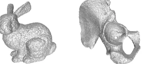
Figure 4:Bunny and hip-bone models. The vertices of the hip-bone model were randomly perturbed using Gaussian noise, while noisy points were added to the vertex set of the bunny model to increase the density. The bumpy but topologically correct outputs shown here were produced by applying our modified power crust algorithm to the noisy point clouds.

Figure 5:View from inside of the hip model. On the left, our proposed method. The feature inside the red circle is the inside view of the small hole in the middle of the hip which can be seen in Figure4. On the right, the original power crust algorithm, which has some artifacts on the interior.

the medial axis then the distance function is well defined on the power crust.

We will prove it is a homeomorphism. Because the power crust is a compact set (it is a finite union of compact sets in this case faces) then we only need to prove that d(_·)

is a continuous, one-to-one and onto mapping. The conti-nuity follows because the distance function to any set is an one-Lipschitz function. The onto condition follows from

dH(Pow(BI∪BO),S)≤ε, that is for any point ˜x∈Sthere

exists at least a power crust point in[x˜−εnx˜,x˜+εnx˜]and given a point in[x˜−εnx˜,x˜+εnx˜]withε≤lfs(S) its closest point onSis ˜x.

The one-to-one condition. Suppose that it is false, it

im-plies that there are two pointsx1andx2 on Pow(BI∪BO)

such that d(x1) = d(x2) or equivalent ˜x1 =x˜2 where x1 andx2 belong to[x˜1−εnx˜1,x˜1+εnx˜1]. Given a pointx∈

[x˜1−εnx˜1,x˜1+εnx˜1]letBcx,ρx∈BIbe a ball which satisfies

dpow(x,Bcx,ρx) = fI(x). LetBx˜1−εnx˜1 ∈BI be a ball which contains the point ˜x1−εnx˜1then we havedpow(x,Bcx,ρx)≤

dpow(x,Bx˜1−εnx˜₁)≤ (ρ+d(x,∂Bx˜1−εnx˜₁))2−ρ2 = O(ε2) whereρ is the radius of the ballBx˜₁₋εnx˜1. From this fact

dpow(x,Bcx,ρx)<O(ε2)we obtain thatd(x,∂Bcx,ρx)≤O(ε), so applying the lemma9to the pointxwe obtain that the angle between the outward normalnx˜ and the vectorcxx~

isO(√ε) and consequently for small enoughr we obtain that this angle is smaller thanπ/2. This means that when

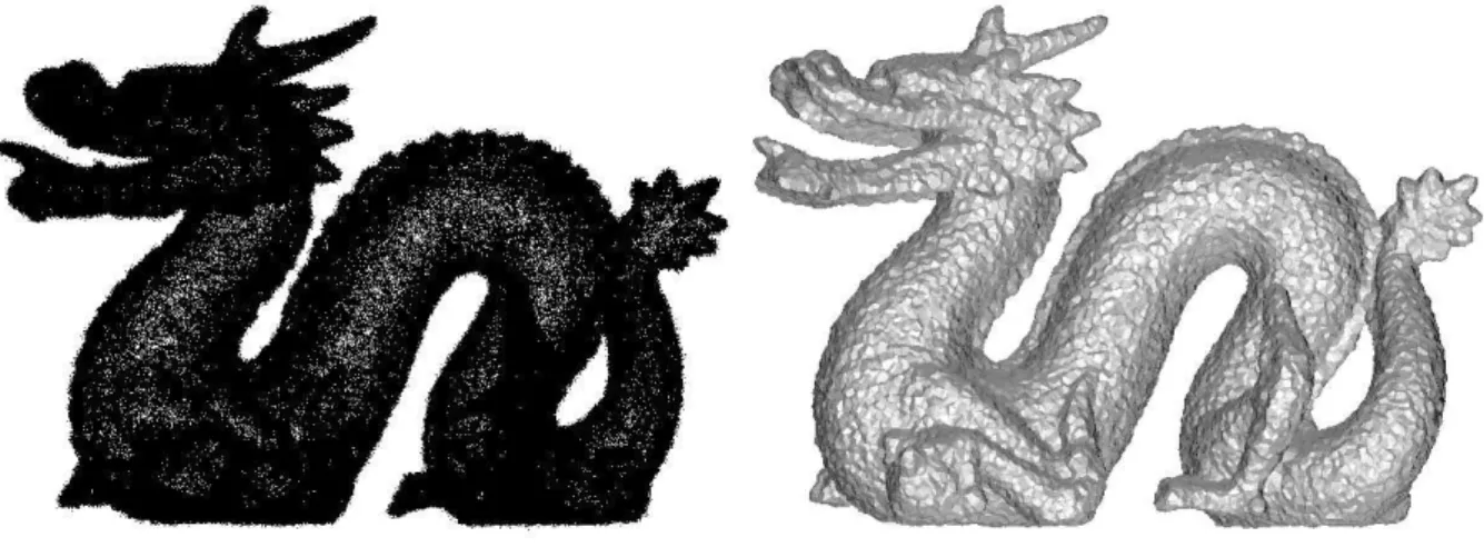
Figure 6:Reconstruction of the dragon model perturbed with Gaussian noise. The perturbed point cloud is shown on the left.

we move the pointxfrom ˜x₁₋εnx˜1 to ˜x1+εnx˜1 along the segment[x˜1−εnx˜1,x˜1+εnx˜1]we have that the function fIis strictly decreasing. The same argument shows that the func-tionfOis strictly increasing.

A power crust points x is characterized by the following equality fI(x) = fO(x). Using that fI(x˜1±εnx˜1)·fO(x˜1∓

εnx˜1)<0 and the functions fIand fOare strictly decreasing and increasing respectively along the interval[x˜1−εnx˜1,x˜1+

εnx˜1]then there exist an unique pointx3on[x˜1−εnx˜1,x˜1+

εnx˜1]such that fI(x3) =fO(x3). From this we conclude that

x1=x2=x3and the functiond(·)is one-to-one.

6. Implementation and Experiments

Since we do not know lfs(S)for a given input surface, we

choose the size of the balls to eliminate by trial and error in each case.

Our experiments were done using an in-house implemen-tation of the power crust algorithm, due to Ravi Kolluri. This code uses Jonathan Shewchuk’s currently unreleased

pyramidcode for Delaunay triangulation. Filtering the

po-lar balls required adding exactly eleven lines of code to the power crust implementation.

We tested the algorithm with several data sets, produced by taking polyhedral models and adding noise. The results are shown in Figures4,5and6. The bunny and the dragon were taken from the Stanford 3D scanning repository, and the hip-bone is from the Cyberware Web site. For the Stan-ford bunny we added four new samples per vertex respec-tively, each perturbed with Gaussian noise. For the hip-bone and the dragon models, which are already fairly large, we just perturbed the input samples. The bunny point set con-sisted of 179,736 points and the reconstruction was

com-puted in less than a minute. The hip-bone set contained 397,625 points and the reconstruction required about 3 min-utes, while the dragon point set contained 875,290 and re-quired about 10 minutes. Experiments were done on a Pen-tium 4, 2.4GHz, with 1Gb of memory.

In each reconstruction we chose the constant δused to filter the polar balls based on the noise level, withδbeing four times the variance of the Gaussian. The noise level in turn was chosen to be less than the smallest feature of the input model, for instance to avoid filling in the hole in the hip-bone or connecting the neck of the dragon to its back.

References

[AB99] AMENTAN., BERNM.: Surface reconstruction by voronoi filtering.Disc. Comput. Geom 22(1999), 481– 502. 1,4

[ABK98] AMENTAN., BERNM., KAMVYSSELISM.: A new voronoi-based surface reconstruction algorithm. In

Proceedings of SIGGRAPH(1998), pp. 415–421. 1 [ACDL00] AMENTAN., CHOI S., DEYT. K., LEEKHA

N.: A simple algorithm for homeomorphic surface re-construction. Internat J. Comput. Geom & Applications

(2000), 125–141. 1

[ACK01a] AMENTA N., CHOI S., KOLLURI R.: The power crust. InProceedings of 6th ACM Symposium on Solid Modeling(2001), pp. 249–260. 1

[ACK01b] AMENTA N., CHOI S., KOLLURI R.: The power crust, union of balls and medial axis transform.

Comput. Geom: Theory & Applications 19(2001), 127– 153. 1,2,3,8,11

[APR02] AMENTA N., PETERS T. J., RUSSELL. A.: Computational topology: Ambient isotopic approxima-tion of 2-manifolds. Theoretical Computer Science

(2002). 3

[BC02] BOISSONNATJ. D., CAZALSF.: Smooth surface reconstruction via natural neighbor interpolation of dis-tance function.Comp. Geometry Theory and Applications

(2002), 185–203. 1

[BMR∗_{99] BERNARDINIF., MITTLEMANJ., RUSHMEIR} H., SILVAC., TAUBING.: The ball-pivoting algorithm for surface reconstruction. IEEE Transactions on Vision and Computer Graphics 5, 4 (1999). 1

[CBC∗_{01] CARRJ. C., BEATSONR. K., CHERRIEJ. B.,} MITCHELLT. J., FRIGHTW. R., MCCALLUM B. C., EVANST. R.: Reconstruction and representation of 3d objects with radial basis functions. InProceedings of SIG-GRAPH(2001), pp. 67–76. 1

[CFG∗_{03] CHENW. S., FUNKEF., GOLINM., KUMAR} P., POONH. S., RAMOSE.: Curve reconstruction from noisy samples.Proc. 19th Annu. Sympos. Comput. Geom.

(2003), 302–311. 2

[CL96] CURLESS B., LEVOYM.: A volumetric method for building complex models from range images. In Pro-ceedings of SIGGRAPH(1996), pp. 303–312. 1 [CL05] CHAZAL F., LIEUTIER A.: Theλ-medial axis.

Graphical Models 67, 4 (2005), 304–331. 2

[DG04] DEYT. K., GOSWAMIS.: Provable surface re-construction from noisy samples . Discrete and Compu-tational Geometry 29, 3 (2004), 15–30. 1,3

[HDD∗_{92] HOPPEH., DEROSET., DUCHAMPT.,} MC-DONALD J., STUETZLE W.: Surface reconstruction from unorganized points. InProceedings of SIGGRAPH

(1992), pp. 71–78. 1

[Kol05] KOLLURI R.: Provably good moving least squares. InProceedings of ACM Symposium on Discrete Algorithms(2005). 2

[Lev03] LEVIND.: Mesh-independent surface interpola-tion. InGeometric Modeling for Scientific Visualization, Brunnett G., Hamann B., Mueller K.„ Linsen L., (Eds.). Springer-Verlag, 2003. 2

[LPC∗_{00] LEVOY M., PULLI K., CURLESS B.,} RUSINKIEWICZS., KOLLERD., PEREIRAL., GINZTON M., ANDERSONS., DAVISJ., GINSBERGJ., SHADEJ., FULKD.: The digital michelangelo project: 3D scanning of large statues. In Proceedings of SIGGRAH (2000), pp. 131–144. 1

Appendix A: Labeling Algorithm

Once we have determined the setP0of polar balls to be re-tained in the noisy version of the power crust algorithm, and

computed their power diagram, the next step of the algo-rithm is to label each of the balls inP0 as an outer or inner ball, thus determining the setsBI andBO. We use exactly

the same labeling algorithm as in the original power crust implementation [ACK01b], but we explain it here for com-pleteness. Then we prove a couple of lemmas which guar-antee that the labeling algorithm is correct. These proofs a similar to analogous proofs in the noise-free case, but again we include them for completeness.

For each sample in the special set Z of vertices of the bounding box, its polar ball is inserted in a queue and la-beled as outer. Then we iteratively propagate the labeling. While the queue is not empty, we remove a ballBpfrom the queue. We examine each of the ballsBqwhose cells neigh-bor that ofBpin the power diagram ofP0. If the intersection betweenBpandBqis at a angle bigger thanπ/4, we assign toBpthe same label asBq. Also we assign the opposite label to the ball of the other pole ofp, if there is one. This process is repeated until there is not a new ball that can be classi-fied as outer or inner. Once we have finished the labeling we determine the faces in Pow(P0)separating inner balls from outer ones.

Lemma 10The angle of intersection between a polar ball

Bc1,ρ1∈BIand a polar ballBc2,ρ2∈BOwithBc2,ρ2∩Bc1,ρ16=

∅isO(r).

ProofWe have that the centerc1andc2ofBc1,ρ1andBc2,ρ2 are in different sides ofS, thus the segment[c1,c2]intersects the surface at a pointx∈S. Let{bi}= [c1,c2]∩∂Bci,ρiwith

i=1,2.

The ballBx,d(x,bi) is inside Bci,ρi which is empty of sam-ples. Then by lemma2we obtain thatd(x,bi) =O(r)lfs(x).

Henced(b1,b2)≤d(x,b1) +d(x,b2)≤O(r)lfs(x), conse-quentlyd(b1,b2)≤O(r)maxx_∈Slfs(x) =O(r)∆1.

LetΠa plane containing the intersection circle between the ballsBc1,ρ1andBc2,ρ2and{z}=Π∩[c1,c2]. Let us bound the distancecitozwe have thatd(ci,z)_≥ρi₋d(b₁,b₂)_≥

ρi−O(r)∆₁. Since thatρi≥lfs(S)/c, then for small enough

rwe have: cos(αi) =d(ci,z) ρi ≥ρi− O(r)∆₁ ρi ≥1−O(r) c∆1 lfs(S)=1−O(r)

Hence we have thatαi=O(r)fori=1,2 and the angle

be-tween the two balls isα1+α2=O(r)

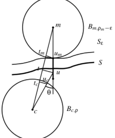
Lemma 11Letεbe smaller than lfs(S). Given a pointuand a ballBc,ρ∈BI (Bc,ρ∈BO)such thatd(u,∂Bc,ρ)≤O(ε)

andu∈Nε, then the angle between the vector~cuand the outward (inward) normal~nu˜isO(√ε).

Proof LetBm,ρm be the outer medial axis ball tangent toS at ˜uand letBc,ρ_∈BIbe a ball such thatd(u,∂Bc,ρ) =O(ε).

LetNεbe a tubular neighborhood ofS. It is easy to see that the ballBm,ρ_m−εis inside the outer solid which is delimited

bySεandΩ, thereforeBc,ρ∩Bm,ρm−ε=∅.

S Sε m um tm uc tc u Bc,ρ Bm,ρm−ε c t θ

Figure 7:The angleθbetween the vectorcu and the normal~ ~nu˜atu˜

.

the projection of u onto the segment cm. Our aim is to find an upper bound for angle between the vectors~cuand

~nu˜ which isθ=∠(m,c,u) +∠(u,m,u) see figure 7. We have the following identities ∠(c,m,u) =arcsin

d(u,t) d(u,m) and∠(m,c,u) =arcsin d(u,t) d(u,c) .

There are three possibilities: t ∈Bm,ρm−ε, t ∈Bc,ρ and

t _∈/ Bm,ρm−εSBc,ρ. When t ∈ Bm,ρm−ε (t ∈ Bc,ρ) us-ing the equations d(u,t) = p

d(u,m)2₋d(t,m)2 and

d(u,t) =p

d(u,c)2₋d(t,c)2 one deduce that d(u,t) _≤ p

(ρ+d(u,∂Bc,ρ))2−ρ2 = O(√ε) when t ∈ Bm,ρ_m−ε

and in the other case t ∈ Bc,ρ we get d(u,t) _≤ q

(ρm+d(u˜,∂Bm,_ρm−ε))2₋ρ2m=O(√ε). From this two

bounds of the distanced(u,t)we obtain that

∠(c,m,u) _≤ arcsin _d(u,t) ρm− q ρ2_m−d(u,t)2 =O(√ε) ∠(m,c,u) _≤ arcsin d(u,t) ρ−p ρ2_−d(u,t)2 =O(√ε)

Now consider t _∈/ Bm,ρ_m−εSBc,ρ. Let tmum with um

∈

∂Bm,ρm be a segment parallel toutand intersecting the

seg-mentscmalso lettcucbe parallel segment totuwithuc∈

∂Bc,ρandtc∈uc. From this we get that

∠(c,m,u) = arcsin _d(um,tm) ρm (19) ∠(m,c,u) = arcsin _d (uc,tc) ρ (20) Due to d(um,tm) _≤ q(ρm₋d(u,∂Bm,_ρm−ε))2₋ρm2 = O(√ε)andd(uc,tc)≤p (ρ−d(u,∂Bc,ρ))2−ρ2=O(√ε)

we obtain that∠(c,m,u) =O(√ε)and∠(m,c,u) =O(√ε)

Corollary 1 The angle of intersection between two balls

Bc1,ρ1∈BIandBc2,ρ2∈BIsuch thatBc1,ρ1∩Bc2,ρ2∩Nε6=∅, isπ−O(√ε).

Proof Take x ∈ Nε∩Bc1,ρ1 ∩Bc2,ρ2. We have that

d(x,∂Bci,ρi) =0 fori=1,2.

Therefore, applying the lemma11 we have the angle be-tween the surface normal~nx˜ and the vector cix~ , is O(√ε) fori=1,2, consequently the angle between the vectorsc~1x andc~2xisO(√ε)and the angle between the tangent planes atxisπ−O(√ε).