Published at CLEEN 2017, Turin, Italy, 21-22 June 2017 – full paper here
A testbed for flexible and energy-efficient resource
management with virtualized LTE-A nodes
N. Iardella
(1,2), G. Nardini
(2), G. Stea
(2), A. Virdis
(2), A. Frangioni
(3), L. Galli
(3), D. Sabella
(4), F. Mauro
(4),
G. Dell’Aera
(4), M. Caretti
(4)(1) DINFO, University of Florence, Italy
(2) Dip. Ing. dell’Informazione, University of Pisa, Italy
(3) Dip. di Informatica University of Pisa, Italy
(4) TIM (Telecom Italia Group), Turin, Italy
Abstract—This paper describes the software architecture and
the implementation of a fully operational testbed that demon-strates the benefits of flexible, dynamic resource allocation with virtualized LTE-A nodes. The testbed embodies and specializes the general software architecture devised within the Flex5Gware EU project, and focuses on two intelligent programs: the first one is a Global Scheduler, that coordinates radio resource allocation among interfering nodes; the second one is a Global Power Man-ager, which switches on/off nodes based on their expected and measured load over a period of minutes. The software framework is written using open-source software, and includes fast, scalable optimization algorithms at both components. Moreover, it sup-ports virtualized BaseBand Units, implemented using OpenAir-Interface, that can run on physical and virtual machines. We pre-sent the results obtained via on-field measurements, that demon-strate the feasibility and benefits of our approach.
Keywords—Coordinated Scheduling, power saving, software framework, Cloud-RAN, testbed, OpenAirInterface, Flex5Gware
I. INTRODUCTION
Cellular networks are evolving towards a dense and hetero-geneous architecture, where macro nodes are used to guarantee ubiquitous coverage and micro cells boost network capacity when needed. In this scenario, operators want to optimize the network-wide energy footprint by switching on micro cells only when needed. Furthermore, inter-cell interference stands as a serious issue, in particular the one from the macro cells to the users served by the micro cells. Coordinated Scheduling (CS) is a Coordinated MultiPoint (CoMP) method that allows nodes to dynamically agree on which frequencies to use in order to re-duce the interference for User Equipments (UEs). In the future, both energy-aware management and inter-cell coordination will leverage flexible hardware-software infrastructures and new paradigms, such as the Virtual Radio Access Network (V-RAN). V-RAN uses general-purpose hardware to implement a node in a virtualized environment and to pool a significant number (i.e., hundreds) of cells in a centralized server, in a so-called “cloud”-RAN (C-RAN) deployment. Such an architec-ture facilitates solving the above problems, since it allows one to design schemes that leverage the availability of information at a centralized point and the low latency of the inter-node (i.e., inter-VM) communications.
The Flex5Gware EU-5GPPP project [1], aims at delivering reconfigurable HW platforms and HW-agnostic software to achieve higher capacity and increased energy efficiency and maximize flexibility in the transition to 5G wireless systems. The project encompasses a wide range of building blocks, from antennas to software architectures. One of the threads of this project aims at researching flexible, effective and efficient
re-source allocation mechanisms in a V-RAN environment, that allow an operator to enhance performance and save energy. This paper presents the software framework underlying the above-mentioned research, which implements a CS server that coordinates virtualized nodes at a fast pace and a power man-agement server that decides which nodes need to be on. We de-scribe the framework, highlighting its flexibility, and the way it interacts with the nodes. We evaluate our framework on a real-life testbed prototype. Our measurements confirm and validate our simulation results [2], showing that CS does increase the channel quality perceived by users connected to micro cells, de-spite the high interference from the macro. To the best of our knowledge, ours is the first prototype to demonstrate this.
The rest of the paper is organized as follows: Section II de-scribes the software framework, whereas Section III dede-scribes the testbed. Section IV describes field results. In Section V we conclude the paper and highlight directions for future work.
II. SOFTWARE FRAMEWORK FOR RESOURCE ALLOCATION Our software framework, outlined in Figure 1 and derived from the general Flex5Gware software architecture [1], consists of two levels: an intelligent program layer on top of the nodes
layer (i.e., eNBs, either macro or micro). The former, whose perspective is network-wide, includes a Monitoring Library
(ML), a database which stores the information to be used by the other components, a Global Scheduler (GS), which embodies the CS, and a Global Power Manager (GPM), whose role is to compute the most energy-efficient network configuration that allows the current load to be carried, by switching off/on nodes. The GPM makes decisions at a relatively slow pace (e.g., tens of minutes), whereas the GS works at sub-second timescales. The node layer contains the eNB components, namely the Re-mote Radio Head (RRH) and the BaseBand Unit (BBU). From the point of view of power management, a physical nodeis vir-tualized through a Local Power Manager (LPM), a software component which is always on. When the GPM wants to switch on/off a node, it contacts its LPM and instructs it to do so. We first describe the general operation of the software framework, and then discuss its implementation in more detail.
Nodes that are switched on register themselves as such on the ML, and start sending their Scheduling Requests (SR) to it. The latter are the number of Resource Blocks (RBs) required to clear their backlog in the current Transmission Time Interval (TTI). Periodically, each node i receives an Allocation Mask
(AM) from the GS, which is a vector of binaries detailing which RBs can/cannot be used by that node. CS is enforced by sending different AMs to different nodes.
The GPM manages a large-scale portion of the network (i.e., several tens or even hundreds of nodes). The network can be
partitioned into CS clusters, each under the supervision of a GS. This is because CS runs at faster timescales, to a point where its
scale becomes the limiting factor. Our CS algorithms can coor-dinate up to 20 nodes every second, or 10 nodes every 100 ms [2]. Therefore, the GPM periodically clusters active nodes, based on their position and radiation information (all of which are static and stored in the ML). For each cluster, it activates an instance of a GS process. The GS polls the ML periodically, re-questing a time average of the SRs of the nodes in its cluster (e.g., on the last 100ms). The ML performs the time average and returns the reply. The GS is aware of the average inter-cell interference that node i does on node j’s users, and uses that in-formation to produce a schedule for all the nodes in its cluster that minimizes the overlapping of RBs for the nodes with the highest mutual interference. When the schedule is done, the GS prepares the AMs and sends them to the nodes.
At a slower timescale (e.g., tens of minutes), the GPM polls the ML for node status and usage statistics of active nodes. Moreover, it retrieves from the ML the expected traffic profiles, that detail what is supposed to happen in the next period based on historical records and context information (e.g., the occur-rence of mass-attendance events, such as a soccer match). Using this information, the GPM prepares a list of nodes to be switched on/off in the next period and the ensuing new cluster-ing, and sends the switching commands to the affected LPMs.
We now describe the implementation of the framework, which is developed in C++ language. All the modules are inde-pendent single- or multi-thread processes that exchange infor-mation via Posix sockets using an ad-hoc application-level pro-tocol which defines the format and the timing of exchanged messages. Intelligent programs are both hardware- and imple-mentation-agnostic: in our testbed, BBUs are embodied by OpenAirInterface software [3], but any other implementation can be supported, as long as it complies to the interfaces. More-over, a LPM knows how to switch on/off both the RRH and the BBU of its node, regardless of whether the latter resides on a physical machine (PM) or a virtual machine (VM). Last, but not least, our framework is flexible: adding a new node only re-quires setting up its own LPM, configuring it with the IP ad-dress and port of the ML, and filling its static information (e.g., position, radiation pattern, etc.) in the ML itself. The intelligent program will then include it in their optimization cycles starting from their respective next period.
A. Monitoring Library
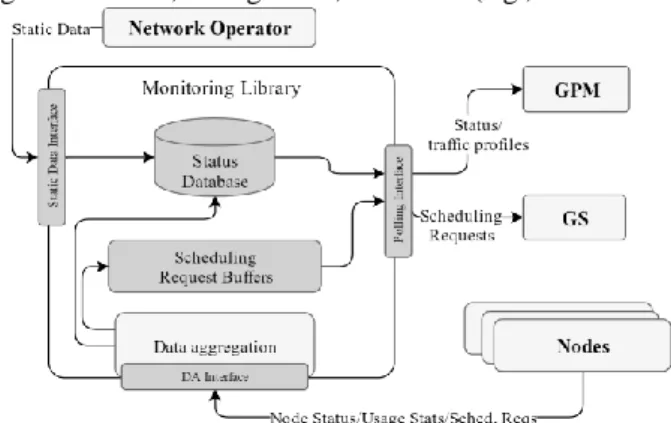
The Monitoring Library (ML) collects the information vided by the nodes and makes it available to the intelligent pro-grams. It serves two main purposes. First, it creates a unified repository for information that may have multiple uses, going beyond those described in this paper. This follows a general trend of endowing cellular networks with data analytics
capabil-ities that can be exploited by different applications, e.g., in a Mobile Edge Computing paradigm [4]. Moreover, it could be easily adapted to work with already available RAN solutions, e.g. SoftRAN [12] or FlexRAN [13]. Second, it solves synchro-nization problems among the entities involved: in fact, if node TTI boundaries are misaligned, the worst that can happen is that the GS will receive as inputs time averages taken on slightly different intervals, whose relative offset is at most one TTI. Similarly, a node may acknowledge a new AM one TTI later than another. However, AMs are typically changed every 100ms or so, hence the performance impact of this is negligible.
The ML must be populated. Some of its data are static, such as node position, radiation pattern, average inter-cell interfer-ence for couple of neighboring nodes, etc. These data must be entered manually by a network operator, which uses a Static Data Interface to do so. The same interface can also be used by the operator to enforce commands (such as manual switch-on of a node) to the LPMs, via the GPM. Among the information that the ML stores we have expected traffic profiles, i.e. curves of required Mbps over time for each node. These are constructed progressively by aggregating the reported usage statistics of ac-tive nodes, and are consulted by the GPM to make switching decisions. Their purpose is twofold: to provide context infor-mation, as already explained, and to substitute actual usage data for nodes that are switched off at the moment (otherwise the GPM would have no basis on which to decide to switch them back on). This information is received through the Data Aggre-gation Interface, together with the nodes Scheduling Requests. The ML also exports a Polling Interface, used by the intelligent programs to obtain the input for their periodic optimization cy-cles. The ML architecture is shown in Figure 2. The Data Ag-gregation Interface is implemented by a passive asynchronous UDP server, since high communication rates are needed and occasional message losses are not overly harmful, which re-ceives the following types of messages: Scheduling Requests coming from the Nodes’ Local Schedulers, Usage Statistics from the Nodes’ Monitoring Agents, and Node Status messages from the Nodes’ Local Power Managers. Scheduling Requests arrive at the rate of one request per TTI, and they are stored in per-node circular local buffers, whose size is a GS period. This serves two purposes: first, an insertion requires one sum and one subtraction, while the extraction of the averaged SR of a node is just an integer division. Therefore, the computational overhead of the most time-critical operations is negligible. Second, the only storage required is one GS period per node, making the framework more scalable. Usage Statistics are ag-gregated on fixed, configurable, time slots (e.g., 10/15 minutes)
and saved in the database. Node Status messages are used to update the database as well. The Polling Interface is implement-ed by two TCP servers that wait for connections from the GS the GPM, since polling is less frequent, but connections need to be reliable. When the GS and the GPM connect to these servers they can ask for Scheduling Requests and Usage Statistics, gregated over suitable past windows. The time filtering and ag-gregation are performed by the ML itself, and the window size is communicated by the requesting intelligent program (e.g., 100ms for GS, 10 minutes for GPM).
B. Global Power Manager
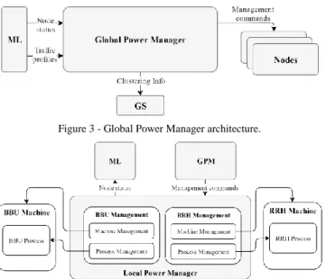
The Global Power Manager (GPM) optimizes power con-sumption by dynamically switching on and off nodes based on the network load. The GPM retrieves network load information and expected traffic profiles using the ML Polling Interface; it runs a power saving algorithm, whose output is a list of nodes whose activity status must be switched; it sends those nodes’ LPMs the appropriate switching commands. Moreover, the GPM activates the CS by starting one GS process per cluster. In doing so, it also informs the GS of the cluster composition. The GPM architecture is shown in Figure 3. The GPM is imple-mented by a single-threaded process, as its operation does not require critical synchronizations, hence concurrency is not re-quired. At the start, the process establishes a TCP connection with the ML and retrieves the addresses of the LPMs of known nodes (whether active or not). Then, it creates a TCP connection with each LPM. Then, it retrieves Usage Statistics and Node
Status periodically using the Polling Interface to the ML, and delivers commands to the LPMs.
In the simplest case, the GPM can be used to turn on all the nodes at boot and reconfigure the network only when explicitly requested by the network operator via override commands committed in the ML. We have provided a sample GPM algo-rithm to go with the implementation. The latter divides each macro cell into areas. An area can be served by more than one eNB: typically, the macro covers all areas, and micros cover a subset of the areas. Some eNB (typically macros) cannot be switched off, some other (e.g., micros) can. The algorithm solves an optimization problem which computes the minimum network-wide power consumption, under the constraint that the traffic demand coming from all areas (as inferred by expected and actual traffic profiles) is satisfied, if possible at all. This re-quires computing the average SINR in each area, which is done taking into account inter-cell interference in all the network. A result of the execution of the GPM algorithm is shown in Figure 4, where switched-off nodes are dark red, and an area is repre-sented by a dot of the same color as its serving node.
C. Local Power Manager
The Local Power Manager (LPM) receives node manage-ment commands from the GPM and controls the BBU and the RRH to activate/deactivate the node itself, i.e. its BBU and RRH. The LPM itself must always be on, because it needs to Figure 3 - Global Power Manager architecture.
Figure 5 - Local Power Manager architecture.
Figure 6 - Sequence diagram of the activation of a BBU/RRH process on a Physical or Virtual Machine by a LPM.
Figure 7 - Global Scheduler architecture. Figure 8 - Sequence diagram for the activation of the framework. Figure 9 – Testbed scenario. Figure 4 - An example of the GPM algorithm execution.
maintain a TCP connection with the GPM to receive manage-ment commands. The LPM needs not be physically co-located with the node: the typical case is a C-RAN architecture, where LPMs are processes running in the cloud, which are cheap in terms of CPU, memory and storage consumption. The only re-quirement is that the LPM is configured with the IP address(es) of the machine(s) hosting the BBU and the RRH. The LPM ar-chitecture is shown in Figure 5. The LPM is highly modular: it includes two distinct management modules, one for the BBU and one for the RRH, assuming that they are separate entities. Since both the BBU and the RRH software is ideally imple-mented by a process running on a machine, both Management Modules have a Process Management component and a Ma-chine Management component. The MaMa-chine Management can control both VMs and PMs. When controlling a PM, the com-ponent uses Wake-on-LAN magic packets to turn it on, and shutdown commands via a SSH connection to turn it off. With VMs, it sends the corresponding commands to the hypervisor. The Process Management component uses SSH connections to send commands to the (virtual or physical) machine’s operating system, to activate the RRH/BBU process after boot, and inter-rupt it before shutting down the machine. The sequence diagram of a node activation is shown in Figure 6 for both the PM and the VM case. The OS-specific part of the LPM is limited to the commands required to activate/interrupt the related processes.
D. Global Scheduler
The Global Scheduler (GS) implements the CS mechanism. Nodes report scheduling requests to the ML, so that the GS can decide an enforce their AMs, namely, which nodes can use which RBs so that the inter-cell interference is minimized. A GS supervises a cluster of interfering nodes. The GPM com-municates the ID of the nodes in the cluster to the GS at the time of activation. The GS architecture is shown in Figure 7.
The GS is a multi-threaded process, since its timing con-straints are tight: a receiver thread polls Scheduling Requests from the ML; a sender thread sends Scheduling Commands to the Local Schedulers; a scheduler thread runs the CS algorithm. The three threads communicate through shared memory and run periodically at different, configurable periods. As CS runs every hundreds or thousands of TTI, the threads are scheduled by the Linux kernel in soft real time. The above design allows one to change the underlying CS algorithm by simply changing the implementation of the scheduler thread. The CS algorithm used in our testbed is the one described in [2]: the latter minimizes the total overlap of subbands among nodes. Each overlapping subband is weighted by the interference coefficient of the two nodes sharing it, so that it is less likely that highly interfering nodes allocate the same subbands. This is achieved by solving a Mixed Integer-Linear problem, whose size is 2C, C being the cluster size. Rather counterintuitively, this formulation allows clusters up to 10 nodes to be coordinated at paces of 100ms. For larger clusters (i.e., up to 20-30 nodes), good suboptimal heuris-tics achieve coordination at periods of 1s. These periods are short enough to capture very fast traffic dynamics.
Most of the CS algorithms proposed in the literature, e.g. [5-8], require information which is unavailable in current cellular networks: for instance, they require UEs to measure and report SINR or CQIs with/without some of the major interferers. Moreover, some of these schemes (e.g., [7,8]), require per-UE
information to be available to the global coordinator, which then allocates resources to single UEs in a multi-cell area. On the other hand, our CS allocates subbands to nodes, leaving to the LSs to enforce per-UE scheduling. This two-level scheduling makes the architecture more scalable and allows for an easy up-grade from already existing nodes.
E. Local Scheduler and Monitoring Agent
The Local Scheduler (LS) resides inside the node’s BBU and allocates RBs to users. On each TTI, the LS computes how many RBs it needs to meet its UEs’ requests. It then sends to the ML the Scheduling Request thus computed, which will be in-cluded in the report to the GS at the next period. When the LS receives a Scheduling Command from the GS, it applies the AM included in it. Nodes check for a new AM on each TTI, just be-fore scheduling their UEs, and keep applying the old one until instructed otherwise. At startup, the default AM is one which enables all RBs. The Monitoring Agent (MA) resides inside the Node’s BBU. It collects Usage Statistics from the Node and sends them periodically to the ML, at periods of tens of seconds or more. The collected Statistics are configurable, and include: number of active UEs, average CQIs of served UEs, average RB occupancy, required MAC-level bandwidth. The MA im-plementation, like the LS’s, depends on the Node implementa-tion. Note that the MA and LS are the only software compo-nents that need be added to the BBUs in order to enable a node to work with our framework.
F. An example
A sequence diagram for our framework is shown in Figure 8: The GPM is launched and queries the ML for Node Status and Usage Statistics. The GPM algorithm decides to turn on a node and it sends a command to its LPM, which activates the node components. Then, the GPM activates a GS instance, communicating to it the ID of the coordinated nodes. When the node is on, its LPM registers it as such into the ML, its MA starts sending Usage Statistics to the ML and its LS starts sending Scheduling Requests to the ML. In the meanwhile, the GS starts polling the ML for scheduling requests and sending scheduling commands to the LS. When a node is not needed anymore, the GPM sends the switch-off command to the LPM, which switches off the node components.
III. DESCRIPTION OF THE TESTBED
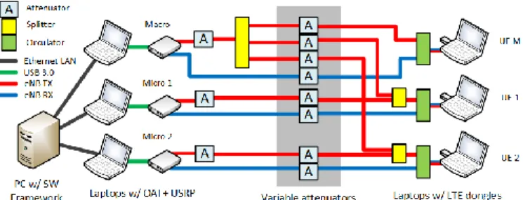
The testbed aims to represent the heterogeneous scenario il-lustrated in Figure 9, consisting of a macro cell and two micro cells. The testbed is outlined in Figure 10. Each node is imple-mented as a single PM, hosting both the BBU and RRH. The BBU is embodied by the OAI software and the RRH runs on a dedicated USRP hardware connected to the PM itself. OAI has been enhanced with our modifications, namely adding a LS and a MA. The local scheduler intercepts the OAI MAC scheduling process, extracts the number of RBs allocated to the UEs for the current TTI, and sends the ensuing SR to the ML. Note that the OAI MAC scheduler allocates RB groups, consisting of three consecutive RBs, starting from the lowest-index ones, hence the resolution of the SR is coarser. The MA for OAI is an in-house statistics collection framework, derived from the ns2-measure software and described in [9]. Each BBU is connected to a RRH, implemented using Ettus USRP B210 boards. UEs are
commercial Huawei E392u-12 dongles connected to three high-end laptops that monitor the UE performance. The core network employed is the Amari-LTE 100 [10], which is a commercial product compatible with OAI. Ad-hoc SIM cards were burned to enable UEs to register with the core network. The intelligent programs, namely the ML, the GS, the GPM, as well as the LPMs for the three nodes, are hosted on a separate laptop. All the nodes and the intelligent programs are in the same Ethernet LAN. In the testbed, all the nodes belong to the same cluster, hence a single GS instance runs at any time.
The test is done with a system bandwidth of 10 Mhz, hence the number of RBs is equal to 50 (17 RB groups, the last of which consisting of two RBs only). UEs are capable of report-ing nine narrowband CQIs. We were unable to determine the
exact correspondence between RB groups and reported CQIs, although it is clear from the standard that the CQI subbands should have the same width (give or take 1 RB), hence 5 or 6 RBs, and that a higher-index subband reports higher-index RBs. Therefore, we cannot match with certainty an RB group to a re-ported narrowband CQI. In order to simplify the monitoring of nodes, each node has a single UE attached to it. This allows us to monitor UEs, instead of nodes, hence does not require us to instrument the BBU software, which is already resource-hungry. Downlink traffic is generated at the nodes using a CBR traffic generator (iperf), at 3, 5 and 7 Mbps.
In order to circumvent instability and synchronization prob-lems between the UEs and the eNBs, the air interface has been channeled in a controlled environment by using wired connec-tions. An 8-way programmable attenuator, splitters and circula-tors were used to emulate inter-cell interference according to the reference scenario. The macro cell generates DL interference for the two micros. UE1 hears both the Macro and Micro 1, but the attenuation on the Macro allows it to attach to Micro 1. The same holds for UE 2, which is attached to Micro 2. Micros do not interfere with each other. Therefore, the SINR of UE 1 and UE 2 are
SINR
x
P
RX,Micro x
P
RX,Macro
N
, where PRX,Micro x is the signal received from 𝑥-th Micro, PRX,Macro is the signal re-ceived from Macro Cell, and 𝑁 is the Noise Power. These val-ues can be controlled and modified using the variable attenua-tor, which allows us to monitor the obtained channel quality us-ing the laptop where the dongle UEs are attached. We used a spectrum analyzer and XCAL (a commercially available benchmarking software running on the UEs), to analyze inter-cell interference between the Macro Cell and the Micro Cells and its effect on CQI values reported by UEs connected to the Micro Cells. A digital clamp meter is used to measure the power consumed by the laptops running the BBUs and the RRHs.IV. FIELD RESULTS
This section describes proof-of-concept field results regard-ing the architecture and the resource allocation algorithms. We first evaluate the framework performance in terms of the com-munication overhead. This is relevant only for comcom-munications related to CS, which occur at sub-second timescales. Those re-lated to power management, instead, occur at much coarser timescales, hence pose no challenge. In particular, we measure the traffic rate of i) Scheduling Requests from the LS to the ML, ii) Scheduling Requests from the ML to the GS and iii) Sched-uling Commands from the GS to the LSs. In our test, each of the three LSs sends one SR per TTI (1 ms) to the ML, as local
scheduling occurs every TTI, as per the standard. The GS was tested using different periods. No deadline misses were ob-served, even when the GS period was brought to an (unrealistic) minimum of 1 ms. Figure 11 shows the traffic rates per node on the channels, at the Ethernet level, against the GS period T. The LS/ML traffic rate per node is independent of T and equal to 416 kbps; the ML/GS and the GS/LS traffic rates are inversely proportional to T. Given that T cannot be expected to be less than 10 ms, the bottleneck is the LS/ML interface. However, even a low-end server should be able to manage several hun-dreds of simultaneous LS/ML flows on a Gigabit Ethernet NIC. This shows that the communications of our framework are well-engineered for a large-scale deployment.
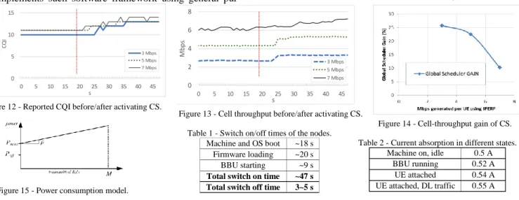
For the node management, we test the switch-on and -off times of the testbed nodes. The former is the time between the switch-on command being sent by the GPM and the cell being up and running. The latter is the time between the command be-ing sent by the GPM and the node machine bebe-ing completely turned off. The switch-on time consists of: i) machine and op-erating system boot time; ii) USRP firmware loading time, and iii) OAI process starting time. The firmware loading is required every time the machine is powered up, since the USRP boards use a SRAM-based FPGA which is reset when powered down. Note that OAI disables all BIOS power-management features, hence no “light” stand-by/sleep/hibernation status can be used in lieu of a complete shut-down. Results in Table 1 show that the switch-on takes less than a minute, and switch-off takes less than five seconds. The largest portion of the switch on time is due to machine/OS booting and firmware loading, both caused by inherent hardware limitations. Using a more advanced setup, with BBUs running on VMs and RRH supporting stand-by, the switch on/off times could be abated by 80%.
We then evaluate how dynamic CS affects the CQIs report-ed by UEs when all nodes transmit their DL traffic. We analyze reported CQI and MAC-layer throughput before and after acti-vating GS. Figure 12 shows the average CQIs reported by UEs attached to Micro Cells (UE 1 and UE 2), before and after the activation of CS, respectively in the 3, 5 and 7 Mbps network load scenario. The red line indicates the start of CS. In all the three scenarios, the reported CQI increases from 10-11 to 14.
Figure 10 - Layout of the testbed.
Figure 11 - Traffic rate, per node, on the three CS interfaces, against the GS period. LS/ML traffic rate is independent of the GS period.
Note that the interference at micro UEs is calibrated so that the latter can actually attach to the micro (instead of the macro). This justifies the fact that the baseline CQIs (10-11) are quite high, and makes it all the more challenging to improve on them. Figure 13 shows the average MAC-layer downlink throughput of UE 1 and UE 2, before and after the activation of CS, with an application-level offered load of 3, 5 and 7 Mbps respectively. As before, the red line states the activation of CS. In all three scenarios, the received data throughput increases. Figure 14 shows the throughput gain in percentage given by CS as offered DL traffic increases. The gain is higher at low traffic rates as CS manages to allocate mutually exclusive, interference-free radio resources for each node. As the offered load increases, CS allo-cates partially overlapping AMs, hence the gain decreases.
As far as power management is concerned, it is difficult, if possible at all, to evaluate the effectiveness of an algorithm that takes into account global, large-scale inter-cell interference, in a testbed with three nodes. However, the testbed serves as a proof of concept for such a mechanism. In a nutshell, the algorithm disables a micro if it has no UE to serve or if the traffic generat-ed by its UEs can be handgenerat-ed over to the Macro Cell. Using the clamp meter, we measured the current absorbed by a node in the following conditions: i) machine on, idle; ii) BBU running; iii) UE attached to the BBU; iv) UE attached and receiving full-buffer downlink traffic. The measurements in Table 2 lead to a “flat” power model, where the level of activity of the node has little, if any, impact on the power consumption. This means that the latter can only be reduced by turning off a node completely. Of course, this holds for our testbed, in which general-purpose machines and entry-level prototyping boards were used, but does not hold in general. Power models available in the litera-ture (e.g., [11]) show that the power consumption depends on the allocated RBs, and that the fixed switch-on power offset will contribute less as technology progresses. Thus, a GPM algo-rithm that optimizes RB allocation is going to make a consider-able difference in the power consumption.
V. CONCLUSIONS
In this work, we described a flexible and scalable software framework that collects network-wide usage statistics, achieves dynamic Coordinated Scheduling at sub-second scales and en-forces power saving node management, all with little customi-zations to the BBU implementation. We also described a testbed that implements such software framework using general
pur-pose machines and entry-level hardware and emulates a simple, yet plausible scenario. The testbed demonstrates two things: first, the computational and communication overhead of the framework is negligible, and the intelligent programs are scala-ble. Second, the dynamic CS and the power saving features do increase the network efficiency, by both using fewer RBs to serve the same traffic and switching off underutilized nodes.
ACKNOWLEDGMENT
This work was partially supported by the European Com-mission in the framework of the H2020-ICT-2014-2 project Flex5Gware (grant agreement no.671563). The authors grateful-ly acknowledge the partial financial support from the University of Pisa, projects "Modelli ed algoritmi innovativi per problemi strutturati e sparsi di grandi dimensioni" (grant PRA_2017_05), and “IoT e Big Data: metodologie e tecnologie per la raccolta e l’elaborazione di grosse moli di dati” (grant PRA_2017_37).
REFERENCES
[1] Flex5Gware website: http://www.flex5gware.eu (accessed Apr. 2017) [2] N. Iardella, et al., "Flexible dynamic Coordinated Scheduling in
Virtual-RAN deployments", IEEE FlexNets Workshop, Paris, May 2017. [3] Navid Nikaein, et al., "OpenAirInterface: A Flexible Platform for 5G
Research", SIGCOMM CCR, 44(5), pp. 33-38, October 2014.
[4] Y. C. Hu et al. “Mobile Edge Computing A key technology towards 5G”, ETSI White Paper, Sept. 2015
[5] G. Li, H. Liu, "Downlink Radio Resource Allocation for Multi-Cell OFDMA System", IEEE TWC, 5(12), pp.3451-3459, Dec. 2006. [6] C. Koutsimanis, G. Fodor, "A Dynamic Resource Allocation Scheme for
Guaranteed Bit Rate Services in OFDMA Networks", Proc. ICC '08, pp.2524-2530, 19-23 May 2008.
[7] M.Y. Arslan, et al. "A Resource Management System for Interference Mitigation in Enterprise OFDMA Femtocells", IEEE/ACM Transactions on Networking, vol.21, no.5, pp.1447-1460, Oct. 2013
[8] G. Nardini, et. al, "Practical large-scale coordinated scheduling in LTE-Advanced networks", Wireless Networks, 22:(1), pp. 11-31, 2016 [9] N. Iardella, et al., "Statistically sound experiments with OAI
Cloud-RAN prototypes", Proc. of CLEEN 2016, Grenoble, FR, May 2016. [10] Amarisoft website: http://www.amarisoft.com (accessed Apr. 2017). [11] Dario Sabella, et al., “Energy Management in Mobile Networks
Towards 5G”, in M.Z. Shakir et al. (eds.), Energy Management in Wireless Cellular and Ad-hoc Networks, Springer, 2016
[12] A. Gudipati et al., “SoftRAN: Software defined radio access network”, ser. HotSDN ’13, 2013.
[13] X. Foukas et al., “FlexRAN: A flexible and programmable platform for software-defined radio access networks” in CoNext, 2016.
Table 1 - Switch on/off times of the nodes. Machine and OS boot ~18 s
Firmware loading ~20 s BBU starting ~9 s
Total switch on time ~47 s
Total switch off time 3~5 s
Table 2 - Current absorption in different states. Machine on, idle 0.5 A
BBU running 0.52 A UE attached 0.54 A UE attached, DL traffic 0.55 A Figure 15 - Power consumption model.
0 5 10 15 0 5 10 15 20 25 30 35 40 45 C Q I s 3 Mbps 5 Mbps 7 Mbps
Figure 12 - Reported CQI before/after activating CS. 0 2 4 6 8 0 5 10 15 20 25 30 35 40 45 M bps s 3 Mbps 5 Mbps 7 Mbps
Figure 13 - Cell throughput before/after activating CS.