Factor forecasting using international targeted predictors: the case of German GDP

(1)

Factor forecasting using

international targeted predictors:

the case of German GDP

Christian Schumacher

Discussion Paper

(2)

Editorial Board: Heinz Herrmann

Thilo Liebig

Karl-Heinz Tödter

Deutsche Bundesbank, Wilhelm-Epstein-Strasse 14, 60431 Frankfurt am Main, Postfach 10 06 02, 60006 Frankfurt am Main

Tel +49 69 9566-0

Telex within Germany 41227, telex from abroad 414431 Please address all orders in writing to: Deutsche Bundesbank,

Press and Public Relations Division, at the above address or via fax +49 69 9566-3077

Internet http://www.bundesbank.de

Reproduction permitted only if source is stated. ISBN 978-3–86558–514–1 (Printversion) ISBN 978-3–86558–515–8 (Internetversion)

(3)

Abstract

This paper considers factor forecasting with national versus factor forecasting with international data. We forecast German GDP based on a large set of about 500 time series, consisting of German data as well as data from Euro-area and G7 countries. For factor estimation, we consider standard principal components as well as variable preselection prior to factor estimation using targeted predictors following Bai and Ng [Forecasting economic time series using targeted predictors, Journal of Econometrics 146 (2008), 304-317]. The results are as follows: Forecasting without data preselection favours the use of German data only, and no additional information content can be extracted from international data. However, when using targeted predictors for variable selection, international data generally improves the forecastability of German GDP.

Keywords: forecasting, factor models, international data, variable selection

(4)

Non-technical summary

Factor models based on large datasets have received increasing attention in the recent macroeconomics literature. Factor models aim at …nding a few representative com-mon factors underlying a large amount of economic activities. Factors can be used as composite coincident business cycle indicators or for forecasting purposes. Particularly for forecasting, factor models based on large data sets have proven useful. A common feature of many applications is that international information is rarely taken into ac-count when forecasting macro variables for a particular ac-country. However, against the background of strong global linkages, variables of one country can have information content for variables of another country in terms of leading-indicator properties, and, in principle, it could be bene…cial to exploit these relationships for forecasting.

In this context, the present paper investigates the information content of interna-tional data for forecasting German GDP with a large factor model, where factor esti-mation is carried out by mean s of principal components analysis. The factor forecasts based on national data are compared to forecasts based on national and international data. The dataset contains about 500 time series, representing the most important Euro-area countries as well as the rest of the G7 in addition to Germany.

As the dataset is quite large and heterogenous, it is likely that at least some of indicators contain little information for future GDP. To account for the di¤erences of informativeness of indicators, we make an attempt to preselect indicators prior to factor estimation. In particular, we employ penalised regression techniques to identify the relevant predictors, that can be used for estimating the factors rather than using the dataset as a whole. To evaluate the procedure, we employ preselection to the national and international datasets together and compare it to preselection applied to national data only.

To assess the information content of the international data, we carry out forecast simulations for German GDP at forecast horizons of up to four quarters. The re-sults show that without preselection the forecasting accuracy of the factor model with national and international data cannot improve over the factor model estimated with national data only. Only the proper preselection of predictors prior to factor estimation improves the forecast performance, if international data is added.

(5)

Nicht-technische Zusammenfassung

Faktormodelle auf Basis großer Datensätze sind Forschungsgegenstand vieler Arbeiten in der jüngeren makroökonomischen Literatur. Mit großen Faktormodellen wird das Ziel verfolgt, eine Vielzahl von ökonomischen Aktvititäten durch eine geringe Zahl von gemeinsamen Faktoren repräsentativ abzubilden, die dann als zusammengesetzte Kon-junkturindikatoren fungieren und als Prädiktoren der Wirtschaftsentwicklung verwen-det werden können. In vielen Studien wird dabei die Prognose des nationalen BIP oder der In‡ationsrate eines bestimmten Landes vornehmlich auf Basis nationaler Daten durchgeführt; internationale Variablen spielen dagegen eine untergeordnete Rolle. Auf-grund weitreichender weltwirtschaftlicher Ver‡echtungen können ausländische Indika-toren jedoch Vorlaufeigenschaften für nationale Variablen aufweisen, die prinzipiell für prognostische Zwecke identi…ziert und verwertet werden sollten.

Vor diesem Hintergrund untersucht das vorliegende Papier den Informationsgehalt internationaler Daten für die Prognose des deutschen BIP mit einem großen Faktor-modell, wobei die Schätzung der Faktoren mit der Hauptkomponentenanalyse erfolgt. Die Faktorprognosen auf Basis deutscher Daten allein werden mit Faktorprognosen auf Basis deutscher und internationaler Daten berechnet und verglichen. Dabei wird ein Datensatz von insgesamt etwa 500 Zeitreihen verwendet, in dem neben Deutschland auch die wichtigsten Länder des Euroraums sowie der Rest der G7 repräsentiert sind. Da bei einem Datensatz dieser Größe und unter Berücksichtigung sehr hetero-gener Länder zu vermuten ist, dass einige Variablen wenig Informationsgehalt für die Entwicklung des deutschen BIP aufweisen, wird auch eine Methode zur Vorauswahl von Prediktoren verwendet. Die Vorauswahl basiert auf einem multiplen Regressions-modell, welches mit speziellen Algorithmen geschätzt wird und die Eliminierung un-wichtiger Variablen ermöglicht. Die daraus resultierende Auswahl von Variablen wird dann für die Faktorschätzung und Prognose verwendet. Ein Vergleich mit den Ergeb-nissen auf Basis des gesamten Datensatzes erlaubt es, Rückschlüsse auf die Leistungs-fähigkeit der Variablenauswahl zu ziehen.

Zur Einschätzung der Relevanz internationaler Daten werden verschiedene Pro-gnosesimulationen mit Prognosehorizonten von bis zu vier Quartalen durchgeführt. Die Ergebnisse zeigen, dass im einfachen Fall ohne ökonometrische Vorauswahl der Daten die Verwendung internationaler und nationaler Daten zugleich die Prognose nicht verbessert im Vergleich zu der Verwendung rein nationaler Daten. Erst durch die angemessene Anwendung der ökonometrischen Variablenvorauswahl verbessert sich die Prognosegüte, wenn internationale Daten zum Datensatz hinzugefügt werden.

(6)

Factor forecasting using international targeted predictors:

The case of German GDP

y

1 Introduction

Large factor models are increasingly important tools for applied research. In particu-lar, they are used for forecasting and as methods to estimate coincident and leading composite indicators, see the survey in Eickmeier and Ziegler (2008), for example. A common feature of many applications is that international information is rarely taken into account when forecasting macro variables for a particular country or region.

In this paper, we investigate the role of international data for forecasting German GDP growth with a large factor model. In previous work, factor models based on national data only have turned out to be useful for forecasting German GDP, see Schu-macher (2007), for example. However, it is well known that Germany is an economy that is highly interrelated with the rest of the world, see for example Eickmeier (2007). Hence, we ask whether international macro variables from large developed economies contain additional relevant information for forecasting German GDP.

In a recursive forecast exercise, we estimate the factors by principal components (PC) following Stock and Watson (2002) based on national data only and compare it to estimates based on national and international data. The dataset contains over …ve hundred indicators covering countries in the Euro area and the remaining G7 in addition to German data. As the dataset is quite large and heterogenous, it is likely that at least some of the indicators are irrelevant for forecasting German GDP. To account for the di¤erences of information content of indicators, we make an attempt to preselect indicators prior to factor estimation. In particular, we follow the proposal of Bai and Ng (2008) and employ penalised regression techniques to identify so-called “targeted predictors”, that can be used for estimating the factors rather than using the dataset as a whole. We employ preselection by targeted predictors to the national and international datasets together and compare it to preselection applied to national data only.

y_{Correspondence:} _{Christian Schumacher, Deutsche Bundesbank, Research Centre,}

Wilhelm-Epstein-Str. 14, 60431 Frankfurt am Main. E-mail: [email protected]. This paper represents the author’s personal opinions and does not necessarily re‡ect the views of the Deutsche Bundesbank. I thank Agnieszka Sosinska for collecting the international dataset, Sandra Eickmeier, Heinz Herrmann and Karl-Heinz Tödter for helpful comments and discussions. The codes used in this paper are written in Matlab. Some of the functions were taken from the Econometrics Toolbox written by James LeSage fromwww.spatial-econometrics.com.

(8)

From an economic point of view, strong trade linkages, cross-border movements of productive factors between integrated economies, or …nancial linkages could justify the information content of variables of one country for another. Hence, the interrelatedness of the major industrialised countries should show up in certain comovements or common factors that have been investigated for example in Kose, Otrok, and Whiteman (2008) and Eickmeier (2008). However, it has rarely been investigated so far whether these factors help to predict better than factors based on national data only. Exceptions are, for example, Brisson et al. (2003) who …nd that Canadian factor forecasts do work better when US information is included, but the forecasts cannot be improved by adding additional time series from other countries, see Brisson et al. (2003), p. 526. Similarly, Banerjee et al. (2005) …nd that US time series matter for forecasting Euro-area variables. Eickmeier and Ng (2009) compare alternative methods based on large-datasets to forecast GDP of New Zealand. However, if we look at the large amount of factor forecast papers published in the recent years, see the surveys in Stock and Watson (2006) and Eickmeier and Ziegler (2008), the general impression is that international data is widely unrecognised or partly neglected in many studies. Thus, there is a gap between factor forecasting investigations and studies concerned with the analysis of international linkages, and taking an international perspective for forecasting with large factor models as in this paper could be worth investigating.

However, recent results from the literature indicate that using more data for factor forecasting does not always improve the predictive ability of models. In particular, Boivin and Ng (2006) …nd that increasing the cross-sectional sample size is not prefer-able, if the additional time series do not contain enough information regarding the factors prevalent in the full dataset. If the idiosyncratic noise is too large or there is cross-correlation between idiosyncratic components, additional variables can indeed distort the factor estimates and lead to inferior forecast performance. According to Boivin and Ng (2006), in the end it is the information content of the additional data what is key for forecasting successfully rather than the sheer size of the dataset. This problem might particularly be relevant also in the present case with a quite large and heterogenous international dataset.

The paper proceeds as follows. Section 2 provides the methodological background of factor forecasting with targeted predictors. Section 3 contains a description of the design of the forecast comparison exercise, as well as empirical results. Section 4 concludes.

(9)

2 Forecasting with factors estimated from targeted

predictors

For forecasting, we follow the standard factor forecast framework introduced by Stock and Watson (2002). According to Bai and Ng (2006), the forecasting model can be speci…ed and estimated as a linear projection of anh-step ahead transformed variable

yh

t+h onto t-dated factor estimatesFbt and a constant and autoregressive lags according

to

y_t+hh = 0Wt+ 0Fbt+"ht+h (1)

fort= 1; : : : ; T h, where indextindicates quarterly time intervals. The variable on the left-hand side of the equation isyh

t+h, which is de…ned as the growth rate of the chosen

time series between periodt and periodt+h, yh

t+h = log(Yt+h=Yt) =

Ph

i=1 log(Yt+i).

In our case,Ytis quarterly German GDP. On the right-hand side, Wt is((p+ 1) 1)

-dimensional and contains the element one as a …rst element andplagged GDP growth terms de…ned as yt = log(Yt=Yt 1). Fbt are (r 1)-dimensional factors estimated by

principal components (PC). and are coe¢ cient vectors, which are estimated by OLS for each forecast horizon h. The out-of-sample forecast for yh

T+h conditional on

information in periodT, namelyWT andFbT, is then given byyh_T_+h_j_T = b0WT+b

0_b

FT.

For the estimation of the factors, we use a large dataset consisting of N stationary time series in Xt. We assume that the variables can be represented as the sum of two

mutually orthogonal components: the common and idiosyncratic components. The common component of each variable is a linear combination of a small number of common factors collected in the r 1 vectorFt. The idiosyncratic components et are

variable-speci…c. Thus, the vector of variables can be represented as

Xt= Ft+et; (2)

for t = 1; : : : ; T. The N r matrix collects the factor loadings of the factors. Concerning the idiosyncratic components, the recent literature, such as Stock and Watson (2002) and Bai and Ng (2002), allows for some non-pervasive cross-sectional correlation of the idiosyncratic components, which leads to the so-called approximate factor model. Furthermore, Stock and Watson (2002) and Bai and Ng (2002) show that even under weak serial correlation and heteroscedasticity of theet and additional

regularity conditions, the factors and factor loadings can be estimated consistently by the method of principal components (PC). Let V denote the N r matrix of the r

eigenvectors corresponding to therlargest eigenvalues of the sample correlation matrix ofXt, which is standardized to have mean zero and unit variance. The PC estimator of

the factors and the factor loadings can be obtained as Fb =XV=pN and b =VpN, where X= (X0

(10)

The consistent estimation of the factors as in Bai and Ng (2002) relies on the factor representation (2), namely, that all variables depend on all the factors. However, it has been shown in Boivin and Ng (2006) that deviations from this representation, where groups of data depend di¤erently on the factors, can deteriorate the forecasting accuracy. This holds, for example, if data is partly uninformative about the factors and, equivalently, contains too much idiosyncratic noise. The forecasting accuracy is also negatively a¤ected if some blocks of data are more informative about one dominant factor than another, and the dominated factor explains the variable we want to predict. Thus, whether adding data helps to improve the forecast performance depends heavily on the information content of the data.

Furthermore, factor estimation by PC aims at maximising the explained variance of the dataset as a whole, and thus neglects that our main aim is predicting onlyyh

t+h. In

this case, certain types of variable preselection might help to choose relevant predictors from the whole set of indicators. Recently, Bai and Ng (2008) have introduced variable preselection by targeting of predictors. Instead of using the full set of indicators to estimateFtfromall theN indicators inXt, Bai and Ng (2008) use penalised regression

techniques to preselect a subset _A of the indicators Xt;A in a …rst step, and then estimate the factors based on this preselected data as in (1). Targeting predictors means that we take into account the relationship between yh

t+h and Xt in order to select the

variables prior to factor estimation. In Bai and Ng (2008), the most promising method for preselection is least-angle regression with elastic net (LARS-EN), which is essentially a penalised regression technique applied to an equation, whereyh

t+h is explained directly

by Xt and by a constant and autoregressive terms. LARS-EN estimation is capable

of removing irrelevant regressors and allowing for shrinkage simultaneously, where EN de…nes the regression problem in terms of shrinkage and elimination following Zou and Hastie (2005), and LARS provides an e¢ cient solution to compute the regression coe¢ cients, see Efron et al. (2004). The regression problem from EN can be described as follows: LetRSS be the residual sum of squares of a regression

yh_t+h = 0Wt+ 0Xt+"ht+h; (3)

where denote the coe¢ cients vector corresponding to the predictors Xt, that are

standardized in the same way as for factor estimation. Then, the EN criterion following Zou and Hastie (2005) is

minRSS+ 1 N X i=1 j ij+ 2 N X i=1 2 i; (4)

where 1 and 2penalise with theL1- andL2-norm of , respectively. The combination

(11)

e¢ cient selection of representatives within groups of highly correlated regressors, and, thus, is superior to using one of the penalties alone following the argumentation in Zou and Hastie (2005), p. 302. LARS is an iterative algorithm that …nds a solving the EN criterion (4), leading to LARS-EN. The algorithm starts with all coe¢ cients set to zero. Then, the most important regressor is selected according to (4) in the …rst iteration. In the next iterations, successively lesser important indicators are selected, while taking into account the correlation with the regressors already in the set_A. For specifying LARS-EN, one …xes the shrinkage parameter 2, and the number of active

regressors N_A included in _A, following Bai and Ng (2008). Thus, a stopping rule for

N_A replaces specifying 1. Note that LARS-EN picks important regressors …rst, thus

the remaining N N_A indicators are the less important ones and are just neglected. More details on the LARS-EN algorithm can be found in appendix A.

3 Empirical evidence for Germany

3.1 Design of the comparison exercise

Below, we evaluate the empirical performance of forecasting of German GDP growth with and without targeted predictors in a framework with a large amount of national and international data. We carry out a variety of recursive forecast comparisons in order to identify the additional information content of the international indicators over the German indicators alone. Furthermore, we investigate the relative advantages of targeted predictors, in particular, we compare the forecast performance of factor models estimated with predictors selected by LARS-EN to the performance of factor models without data preselection. Preselection is applied to the two di¤erent datasets: the national data only as well as the whole dataset including the national and international data. Thus, we take into account that preselection of national data alone could also yield sizeable gains in terms of forecast accuracy, and not only adding international data.

Data The national German data consists of quarterly GDP growth as well as 123

quarterly indicators, and is taken from Schumacher (2007). The dataset includes GDP expenditure components as well as gross value added by sectors. It also contains in-dustrial production, received orders and turnover, disaggregated by sectors. Labour market variables considered are employment, unemployment and wages. Several dis-aggregated price indices and de‡ator are considered, as well as …nancial time series such as interest rates and spreads. Additionally, we use ifo survey time series such as business situation and expectations, assessment of stocks and capacity utilisation, and other series.

(12)

The international dataset contains indicators from the main Euro-area countries and the remaining G7 countries. Euro-area countries in the dataset are Austria, Belgium, Finland, France, Italy, Netherlands, and Spain. From the remaining G7 countries, we include Canada, UK, Japan, and the USA. Concerning coverage, the Euro-area data is similar to the dataset in Eickmeier (2008), and the G7 data used here was selected accordingly. Generally, selection of variables is done such that the economies are represented in a relatively balanced way, although it is generally impossible to generate a fully balanced dataset, see Eickmeier (2008), p. 9, for example. Furthermore, the coverage is similiar to that of the German dataset, so the most of the groups of national data are also represented in the international data.

Overall, we have 531 variables in the dataset. The initial period of the dataset is 1980Q3, and the …nal period is 2004Q4. The time series are seasonally adjusted and corrected for outliers. Moreover, since the PC estimation of the factors requires stationary time series, non-stationary time series were appropriately di¤erenced. More details on the dataset can be found in the data appendix C.

Recursive estimation and forecasting To evaluate the alternative forecasts, we consider the evaluation period from 1997Q1 to 2004Q4. For factor estimation, the initial period of the dataset is always 1980Q3, wheareas the …nal period is recursively expanded from 1996Q4 onwards until the end of the sample. For each period in the evaluation sample, we compute forecasts with a horizon of h= 1; : : : ;4. As the direct forecast equation (1) is horizon-dependent, we have to reestimate its coe¢ cients for every recursion and horizon. When employing targeted predictors, we also preselect the necessary indicators every recursion and horizon, as also LARS-EN is horizon-dependent.

To evaluate the forecasts, we compute root mean-squared forecast errors (RMSE). In the tables below, we compare factor forecasts to two benchmarks: the in-sample mean of GDP as well as the autoregressive (AR) model, both estimated recursively. All RMSE of the factor forecasts and the AR model are computed relative to the RMSE of the in-sample mean. Relative RMSE smaller than one indicate informative forecasts with respect to the naive in-sample mean benchmark. The AR model is speci…ed as a direct multi-step equation including a constant and estimated with a maximum lag order of four, and the lag order is speci…ed by using the Bayesian information criterion (BIC).

Speci…cation issues Regarding the speci…cation of the number of factors r, we consider alternative …xed speci…cations as well as simulations with speci…cations based on information criteria, that we apply recursively. For this purpose, we employ the criterion ICp2 from Bai and Ng (2002) with a maximum number of factors equal to r = 6. Autoregressive terms are included with up to four lags, and the lag order

(13)

determination is done by applying the BIC again. As an alternative, we also employ the BIC to specify simultaneously the lag orders as well as the number of factors, following Stock and Watson (2002), for example.

Concerning the targeting of predictors, we also compare a variety of auxiliary parameters in LARS-EN: The sample size contains alternatively N_A _{2 f}30;60;90;

120;180;240;300_g variables, whereas we allow for di¤erent values of 2 according to 2 2 f1:5;0:5;0:25;0:10g. Note that Bai and Ng (2008) choose N = 30 and 2 = 0:25

suitable for their US dataset consisting of132 predictors. As the national and interna-tional dataset considered here is much larger and contains data from very heterogeneous countries, and it could be advisable to allow for alternative parameter settings.

In order to circumvent potential mis-speci…cation of the various auxiliary para-meters, we also incorporate pooling over all above mentioned combinations of mod-els consisting of N_A _{2 f}30;60;90;120;180;240;300_g, 2 2 f1:5;0:5;0:25;0:10g, and r = 1; : : : ;6. A similar strategy in a VAR model context has been applied recently, for example, by Clark and McCracken (2008) and Garratt et al. (2009), where fore-cast combinations over di¤erent speci…cations of vector autoregressive (VAR) models have proven useful for forecasting under model uncertainty. As weighting schemes, we use equal-weight pooling, the median as well as performance-based pooling, where the previous four-quarter RMSE of each model determines its weight, see again Clark and McCracken (2008) for a successful implementation of these simple combination schemes.

3.2 Results

Table 1 contains forecast results for alternative factor models and forecast horizons up to four, where speci…cation was carried out recursively. In column I, the information criteria by Bai anf Ng (2002) were employed to determine the number of factors. In column II, results based on BIC model selection for lag lengths and the number of factors are presented. Results are presented pairwise, where in the …rst row forecast results based on models estimated using German data only are presented, and in the second row, results based on the merged German and international data are presented, see column ‘data’. Furthermore, panel A of the table contains results based on the respective full datasets without preselection, and panel B contains results based on various speci…cations of LARS-EN with respect to the parameter 2 and sample size N_A.

The overall performance indicates that forecasts are at best informative up to three quarters, as the relative RMSEs are larger than one in almost all of the cases, in line with previous results from Schumacher (2007). Regarding the information content of international versus national data, the …ndings depend on the speci…cation. Without variable preselection, applying the standard factor-based forecasts proposed by Stock

(14)

Table 1: Forecast results with German and international data, information criteria model selection

data LARS-EN horizon horizon

2 NA 1 2 3 4 1 2 3 4

I. Bai/Ng (2002) spec II. full BIC spec A. no preselection ger - 124 0.97 1.02 1.09 1.12 0.96 1.02 1.01 1.07 ger+int - 531 0.99 1.07 1.17 1.18 0.96 1.04 1.10 1.17 B. LARS-EN preselection ger 0:25 30 1.03 0.93 1.03 0.95 0.93 0.96 1.02 1.00 ger+int 0:25 30 0.92 0.87 0.99 1.00 0.94 0.90 1.00 0.98 ger 0:25 60 0.95 0.93 1.07 1.11 1.00 0.97 0.99 1.07 ger+int 0:25 60 0.81 0.97 0.94 1.07 1.12 0.95 0.95 1.04 ger 0:25 90 0.91 1.03 1.08 1.04 0.98 0.93 1.01 1.06 ger+int 0:25 90 0.87 0.95 0.87 1.05 0.98 0.94 0.91 0.99 ger 0:25 120 0.94 1.04 1.09 1.11 0.97 1.07 1.01 1.06 ger+int 0:25 120 0.86 0.98 0.94 1.07 0.91 0.98 0.97 1.04 ger 0:25 124 0.97 1.02 1.09 1.12 0.96 1.02 1.01 1.07 ger+int 0:25 180 0.86 0.96 1.01 1.14 0.93 0.93 1.00 1.09 ger+int 0:25 240 0.95 1.00 1.11 1.17 0.88 0.96 1.08 1.14 ger+int 0:25 300 0.97 1.02 1.13 1.16 0.95 1.01 1.08 1.15 C. AR benchmark GDP - - 0.99 0.99 1.01 1.03

Note: The entries in the table are relative RMSEs of the factor models relative to the RMSE of the forecast equal to the in-sample mean. The mean is computed reccursively every subsample.

(15)

and Watson (2002), adding international data cannot improve or can even deteriorate the forecast performance, see panel A. If LARS-EN is employed to preselect variables (panel B), we …nd in many cases an improvement of the forecast performance by adding international to national data. However, this result depends on the number of vari-ables included. If up to N_A = 60 variables are selected, the results vary over the forecast horizon, and the RMSE ranking changes between international and national factor models. However, after increasing the number of preselected variables further, we …nd more cases, where international data helps to improve forecast performance. However, this generally holds for informative forecasts only, i.e. with a relative RMSE smaller than one. For increasing model size N_A 180, international data only helps for forecasts of horizon one, and are independent of the choice of dataset mostly un-informative.1 _{If we search for the best performance in our results, we …nd that using}

international and national data together with Bai and Ng (2002) information criteria and LARS-EN with N_A = 90;120 variables do best. This is a relatively stable result over the forecast horizons. The advantages of using international data are more pro-nounced, if the Bai and Ng (2002) information criteria are employed for selecting the number of factors. Comparing columns I and II, the BIC works overall a little bit worse than the Bai and Ng (2002) information criteria.2 _{Overall, there is some speci…cation}

uncertainty with respect to the appropriate auxiliary parameter N_A that a¤ects the forecast performance. Note that we have also varied the LARS-EN parameter 2. In

line with …ndings by Bai and Ng (2008), this parameter has a negligible e¤ect on the forecast performance, as can be veri…ed in the appendix B.

To consider speci…cation uncertainty to a wider extent as before, we now provide pooling results, where the combinations of forecasts include models with all di¤erent speci…cations concerning the number of factors, LARS-EN auxiliary parameters and so on, thus following the recent literature on forecasting under model uncertainty, see Clark and McCracken (2008) and Garratt et al. (2009). Table 2 contains the RMSE results based on pooling, where we di¤erentiate between pooling over national data only on the one hand, and pooling over models with national and international data on the other, see the …rst column of table 2. Furthermore, we pool over model sets containing only models estimated with the whole dataset without preselection, see panel A. In panel B, we pool over models that were estimated with preselected data. Within these model sets, we pool over speci…cations of LARS-EN and the number of factors. The results show strong evidence in favour of the relevance of international

1_{Note that the German dataset includes}₁₂₄ _{time series only, and preselection from larger sample}

sizes can only be applied to the merged national and international dataset.

2_{If we look at the number of factors recursively selected by the two speci…cation schemes, it turns}

out that BIC (column II) methods selects only a few factors, often only one factor. On the other hand, the Bai and Ng (2002) criteria select in most of the cases between 4 and 6 factors, and thus extract a richer factor structure that seems.contain additional information for future GDP growth.

(16)

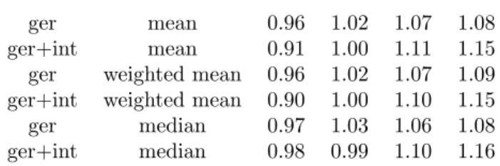
Table 2: Forecast results for factor models with German and international data, pooling over many speci…cations

horizon quarter

data weighting 1 2 3 4

A. pooling of models with full data only

ger mean 0.96 1.02 1.07 1.08 ger+int mean 0.91 1.00 1.11 1.15 ger weighted mean 0.96 1.02 1.07 1.09 ger+int weighted mean 0.90 1.00 1.10 1.15 ger median 0.97 1.03 1.06 1.08 ger+int median 0.98 0.99 1.10 1.16 B. pooling of models with LARS-EN preselection

ger mean 0.94 0.97 1.05 1.05 ger+int mean 0.84 0.88 0.99 1.03 ger weighted mean 0.94 0.98 1.04 1.04 ger+int weighted mean 0.85 0.87 0.97 1.01 ger median 0.96 1.00 1.06 1.06 ger+int median 0.87 0.90 1.00 1.06

Note: The entries in the table are relative RMSEs of the factor models relative to the RMSE of the forecast equal to the in-sample mean. The mean is computed reccursively every subsample. In Panel A, combinations are computed over models that have been estimated based on the full data, whereas Panel B contains model results based on preselected data by LARS-EN.

(17)

data. In almost all cases, where relative RMSE are smaller than one, factor models based on international data clearly outperform factor models based on national data only. Concerning preselection, we …nd that pooling over models based on the whole data is clearly inferior to pooling of models with preselected data. In most of the cases for horizons larger than two, the forecasts without preselection are almost entirely uninformative, indicated by relative MSE larger than one. Thus, international data and preselection of data together yield the best results overall. The weighting schemes have only little impact on the pooling results, and the simple equal-weight average over the models is doing quite well. Compared to the results based on information criteria, we …nd that pooling is only slightly worse than the best speci…cation in table 1.

4 Conclusions

This paper compares factor forecasts based on national data only with factor forecasts based on national and international data for the German economy. We …nd that principal components based on the whole set of national and international indicators do not contain additional information for future German GDP growth. However, if we follow Bai and Ng (2008) and preselect variables prior to factor estimation using LARS-EN, international data provides additional information content and generally improves over forecasts based on national data. Thus, the results support the use of “targeted predictors” from a large set of national and international data. In line with earlier …ndings from Boivin and Ng (2006), more data is not always better for factor forecasting, and only careful preselection of variables, in our case LARS-EN, helps exploiting the additional information content from the large and heterogenous dataset including international variables.

References

[1] Banerjee, A., M. Marcellino, I. Masten (2005), Leading indicators for the Euro area in‡ation and GDP growth, Oxford Bulletin of Economics and Statistics 67, 785-814.

[2] Bai, J., S. Ng (2002), Determining the Number of Factors in Approximate Factor Models, Econometrica 70, 191-221.

[3] Bai, J., S. Ng (2006), Con…dence Intervals for Di¤usion Index Forecasts and In-ference for Factor Augmented Regressions, Econometrica 74, 1133-1150.

[4] Bai, J., S. Ng (2008), Forecasting economic time series using targeted predictors, Journal of Econometrics 146, 304-317.

(18)

[5] Boivin, J., S. Ng (2006), Are More Data Always Better for Factor Analysis, Journal of Econometrics 132, 169-194.

[6] Brisson, M., B. Campbell, J.W. Galbraith (2003), Forecasting Some Low-predictability Time Series Using Di¤usion Indices, Journal of Forecasting 22, 515-531.

[7] Clark, T., M. McCracken (2008), Averaging Forecasts from VARs with Uncertain Instabilities, Journal of Applied Econometrics, forthcoming.

[8] Efron, B., T. Hastie, I. Johnstone, R. Tibshirani (2004), Least angle regression, Annals of Statistics 32, 407-499.

[9] Eickmeier, S. (2007), Business cycle transmission from the US to Germany – a structural factor approach, European Economic Review 51, 521-551.

[10] Eickmeier, S. (2008), Comovements and heterogeneity analyzed in a non-stationary dynamic factor model, Journal of Applied Econometrics, forthcoming. [11] Eickmeier, S., T. Ng (2009), Forecasting national activity using lots of interna-tional predictors: an application to New Zealand, Deutsche Bundesbank Discus-sion Paper, Series 1: Economic Studies, No. 11/09.

[12] Eickmeier, S., C. Ziegler (2008), How successful are dynamic factor models at fore-casting output and in‡ation? A meta-analytic approach, Journal of Forefore-casting 27, 237-265.

[13] Fagan, G., J. Henry, R. Mestre (2001), An area-wide model (AWM) for the euro area, ECB Working Paper 42.

[14] Fagan, G., J. Henry, R. Mestre (2005), An area-wide model for the euro area, Economic Modelling 22, 39-59.

[15] Garratt, A., E. Mise, G. Koop, S. Vahey (2009), Real-time Prediction with UK Monetary Aggregates in the Presence of Model Uncertainty, Journal of Business and Economic Statistics, forthcoming.

[16] Kose, M.A., C. Otrok, C.H. Whiteman (2008), Understanding the evolution of world business cycles, Journal of International Economics 75, 110–130.

[17] Schumacher, C. (2007), Forecasting German GDP using alternative factor models based on large datasets, Journal of Forecasting 26, 271-302.

[18] Stock, J., M. Watson (2002), Macroeconomic Forecasting Using Di¤usion Indexes, Journal of Business & Economic Statistics 20, 147-162.

(19)

[19] Stock, J., M. Watson (2006), Forecasting with Many Predictors, in: Elliot, G., Granger, C., Timmermann, A. (eds.), Handbook of Economic Forecasting, Vol 1, 515-554.

[20] Watson, M. (2003), Macroeconomic Forecasting Using Many Predictors, in: M. Dewatripont, L. Hansen and S. Turnovsky (eds.), Advances in Economics and Econometrics, Theory and Applications, Eight World Congress of the Econometric Society, Vol. III, 87-115.

[21] Zou, H., T. Hastie (2005), Regularization and variable selection via the elastic net, Journal of Royal Statistical Society Series B, 67, 301-320.

A

The LARS-EN algorithm

LARS-EN proceeds in two steps: First, the EN criterion is reformulated as a simple criterion based on transformed data that takes into account the ENL2-penalty. Second,

the LARS algorithm is employed to …nd the penalized regression coe¢ cients. The elastic net (EN) criterion

minRSS+ 1 N X i=1 j ij+ 2 N X i=1 2 i; (5)

can be written as a simpler criterion by setting

X+= (1 + 2) 1=2 X p 2IN ! and y+= y 0N ! ; (6) leading to minRSS++_p 1 1 + 2 N X i=1 j ij; (7)

whereRSS+is the residual sum of squares from a regression ofy+ onX+, see Zou and Hastie (2005), p. 304. This criterion is a so-called LASSO (“least absolute shrinkage and selection operator”) criterion and can be solved by least-angle regression (LARS) applied to transformed data y+ and X+.

Let the part of y+ explained by the selected predictors be denoted as bA. The subset_A of indices de…nes selection of dataX+_A = ( sjx+j )j2A. The signssj equal

1 according tosj =signfbcjg forj 2 A. The current correlationsbcj are taken from

(20)

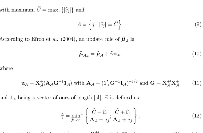
with maximum Cb = maxjfjbcjjgand

A =nj :_j_bcjj=Cb

o

: (9)

According to Efron et al. (2004), an update rule of _b_A is

bA+ = bA+buA; (10)

where

u_A=X+_A(A_AG 11_A) with A_A = (10_AG 11_A) 1=2 and G=X+_A0X+_A (11)

and 1_A being a vector of ones of length_jAj. _b is de…ned as

b=min j2Ac + ( b C _bcj A_A aj ; Cb+bcj A_A+aj ) ; (12)

where aj is the j-th element froma=X+0uA. “min+” minimizes over positive entries only. If the minimizing index j in (12) is denoted as bj, then the update of the active set_A+ becomes A [ fbjg.

The LARS algorithm starts with no variables selected, implying _b_A = 0T and

A=_?. In the next iteration, the element of the indicators with maximum correlation b

cj from (8) is chosen. The update rule (10) provides the new …tted value of y+, b_A₊.

At each step, the _b in LARS is chosen so that the algorithm proceeds equiangularly between the variables in the most correlated set in the “least angle” direction until the next variable is found. If we end after N_A steps, we will have an active set of N_A

predictors, and all the otherN N_A coe¢ cients are zero. Thus, for specifying LARS-EN, we have to …x 2 iny+ and X+ and choose a maximum number of variables NA in terms of the stopping rule for the LARS algorithm. Thus, in LARS-EN, specifying the penalty parameter 1 is replaced by specifying the stopping rule NA. Note that we employ LARS-EN only for selecting N_A predictors, that enter the dataset for PC estimation of the factors, whereas we are not interested in the parameter estimates of

.

B

Empirical results for alternative speci…cations

Table 3 contains forecast results based on the same settings as the results in table 1, but with 2 = 1:5. Other values yielded similar results and are not reported here. The

results indicate no major di¤erences with the new 2. Thus, we can con…rm the main

(21)

Table 3: Forecast results with German and international data, information criteria model selection

data LARS-EN horizon horizon

2 NA 1 2 3 4 1 2 3 4

I. Bai/Ng (2002) spec II. full BIC spec A. no preselection ger - 124 0.97 1.02 1.09 1.12 0.96 1.02 1.01 1.07 ger+int - 531 0.99 1.07 1.17 1.18 0.96 1.04 1.10 1.17 B. LARS-EN preselection ger 1:50 30 0.94 0.98 1.02 0.95 0.90 0.98 1.00 1.07 ger+int 1:50 30 0.94 0.88 1.01 0.99 0.93 0.86 1.01 0.98 ger 1:50 60 0.97 0.93 1.11 1.09 1.04 0.95 1.00 1.06 ger+int 1:50 60 0.85 0.95 0.99 1.05 1.03 1.03 1.00 1.09 ger 1:50 90 0.91 1.01 1.11 1.06 0.99 0.94 1.02 1.07 ger+int 1:50 90 0.89 0.96 0.87 1.04 0.95 0.98 0.94 1.02 ger 1:50 120 0.95 1.01 1.09 1.14 0.98 0.94 1.02 1.07 ger+int 1:50 120 0.81 0.97 0.95 1.06 0.88 0.98 0.99 1.02 ger 1:50 124 0.97 1.02 1.09 1.12 0.96 1.02 1.01 1.07 ger+int 1:50 180 0.85 0.96 1.01 1.12 0.91 0.97 1.00 1.08 ger+int 1:50 240 0.96 0.99 1.12 1.17 0.89 1.01 1.08 1.14 ger+int 1:50 300 0.97 1.02 1.13 1.16 0.94 1.01 1.09 1.15 C. AR benchmark GDP - - 0.99 0.99 1.01 1.03

Note: The entries in the table are relative RMSEs of the factor models relative to the RMSE of the forecast equal to the in-sample mean. The mean is computed reccursively every subsample.

(22)

C

Data appendix

C.1 General features of the data

Overall, we have 531 variables in the dataset. The initial period of the dataset is

1980Q3, and the …nal period is2004Q4.

The national German data consists of quarterly GDP growth as well as 123 quar-terly indicators, and is taken from Schumacher (2007). The selection of the data follows the seminal work by Stock and Watson (2002), and aims at an as broad as possible coverage of the variables. The dataset includes GDP expenditure components such as consumption and …xed capital formation, as well as gross value added by sectors. It also contains industrial production, received orders and turnover, disaggregated by sec-tors. Labour market variables considered are employment, unemployment and wages. Several disaggregated price indices and de‡ator are considered, as well as …nancial time series such as interest rates and spreads. Additionally, we use ifo survey time series such as business situation and expectations, assessment of stocks and capacity utilization, and other series.

The international dataset contains 407 indicators from the main euro area and the remaining G7 countries. Euro area countries in the dataset are Austria, Belgium, Finland, France, Italy, Netherlands, and Spain. We also include the remaining G7 countries Canada, Great Britain, Japan, and the USA. Concerning coverage, the euro area data is similar to the dataset in Eickmeier (2008), and the G7 data used here was selected accordingly. Generally, selection of variables is done such that the economies are represented in a relatively balanced way, although it is generally impossible to generate a fully balanced dataset, see Eickmeier (2008), p. 9, for example. Furthermore, the coverage is similar to that of the German dataset, so the most of the groups of national data are also represented in the international data.

Prior to estimation, the data has been preprocessed in several ways. Natural log-arithms were taken for all time series except interest rates, unemployment rates, and capacity utilization. Most of the time series taken from the above sources are already seasonally adjusted. Remaining time series with seasonal ‡uctuations were adjusted using Census-X12. Extreme outlier correction was done using the procedure proposed by Watson (2003). Large outliers are de…ned as observations that di¤er from the sam-ple median by more than six times the samsam-ple interquartile range, see Watson (2000), p. 93. The identi…ed observation is set equal to the respective outside boundary of the interquartile. Following Stock and Watson (2002), non-stationary time series from the dataset were appropriately di¤erenced, as the principal components (PC) estimation of the factors requires stationary time series. To eliminate scale e¤ects, the series were centered around zero mean and standardized to have unit variance.

(23)

section C.3 provides the same information related to the international dataset.

C.2 German data

The whole data set for Germany contains124 quarterly series including GDP. Some of the time series for uni…ed Germany are available only for the time period after1991. In order to obtain longer samples, the time series of West Germany and uni…ed Germany were combined after rescaling the West German data to the uni…ed German time series.3 _{The national accounts data for West and uni…ed Germany are both measured}

according to the ESA 95 (European System of National Accounts).

Use of GDP and gross value added

1. gross domestic product

2. private consumption expenditure 3. government consumption expenditure

4. gross …xed capital formation: machinery & equipment 5. gross …xed capital formation: construction

6. gross …xed capital formation: other 7. exports

8. imports

9. gross value added: mining and …shery

10. gross value added: producing sector excluding construction 11. gross value added: construction

12. gross value added: wholesale and retail trade, restaurants, hotels and transport 13. gross value added: …nancing and rents

14. gross value added: services

Prices

1. consumer price index 2. export prices

3. import prices 4. terms of trade 5. de‡ator of GDP

3_{This procedure avoids modelling regime shifts and follows numerous empirical studies based on}

German data. For example, the euro area-wide model proposed by Fagan et al. (2005) relies on German time series that are linked as described above, see Fagan et al. (2001), p. 52.

(24)

6. de‡ator of private consumption expenditure 7. de‡ator of government consumption expenditure 8. de‡ator of machinery & equipment

9. de‡ator of construction

Manufacturing turnover, production and received orders

1. production: intermediate goods industry 2. production: capital goods industry

3. production: durable and non-durable consumer goods industry 4. production: mechanical engineering

5. production: electrical engineering 6. production: vehicle engineering

7. export turnover: intermediate goods industry 8. domestic turnover: intermediate goods industry 9. export turnover: capital goods industry

10. domestic turnover: capital goods industry

11. export turnover: durable and non-durable consumer goods industry 12. domestic turnover: durable and non-durable consumer goods industry 13. export turnover: mechanical engineering

14. domestic turnover: mechanical engineering 15. export turnover: electrical engineering industry 16. domestic turnover: electrical engineering industry 17. export turnover: vehicle engineering industry 18. domestic turnover: vehicle engineering industry

19. orders received by the intermediate goods industry from the domestic market 20. orders received by the intermediate goods industry from abroad

21. orders received by the capital goods industry from the domestic market 22. orders received by the capital goods industry from abroad

23. orders received by the durable and non-durable consumer goods industry from the domestic market

24. orders received by the durable and non-durable consumer goods industry from abroad 25. orders received by the mechanical engineering industry from the domestic market 26. orders received by the mechanical engineering industry from abroad

27. orders received by the electrical engineering industry from the domestic market 28. orders received by the electrical engineering industry from abroad

29. orders received by the vehicle engineering industry from the domestic market 30. orders received by the vehicle engineering industry from abroad

(25)

Construction

1. orders received by the construction sector: building construction 2. orders received by the construction sector: civil engineering 3. orders received by the construction sector: residential building

4. orders received by the construction sector: non-residential building construction 5. man-hours worked in building construction

6. man-hours worked in civil engineering 7. man-hours worked in residential building 8. man-hours worked in industrial building 9. man-hours worked in public building 10. turnover: building construction 11. turnover: civil engineering 12. turnover: residential building 13. turnover: industrial building 14. turnover: public building

15. production in the construction sector

Surveys

1. business situation: capital goods producers

2. business situation: producers durable consumer goods 3. business situation: producers non-durable consumer goods 4. business situation: retail trade

5. business situation: wholesale trade

6. business expectations for the next six months: producers of capital goods

7. business expectations for the next six months: producers of durable consumer goods 8. business expectations for the next six months: producers of non-durable consumer goods 9. business expectations for the next six months: retail trade

10. business expectations for the next six months: wholesale trade 11. stocks of …nished goods: producers of capital goods

12. stocks of …nished goods: producers of durable consumer goods 13. stocks of …nished goods: producers of non-durable consumer goods 14. capacity utilization: producers of capital goods

15. capacity utilization: producers of durable consumer goods 16. capacity utilization: producers of non-durable consumer goods

(26)

Labour market

1. residents 2. labour force 3. unemployed

4. employees and self-employed 5. employees

6. self-employed

7. volume of work, employees and self-employed 8. volume of work, employees

9. hours, employees and self-employed 10. hours, employees

11. productivity, per employee 12. productivity, per hour

13. wages and salaries per employee 14. wages and salaries per hour

15. wages and salaries, excluding employers’social security contributions 16. unit labour costs, per production unit

17. unit labour costs, per production unit, hourly basis 18. short-term employed

19. vacancies

20. unemployment rate

Interest rates, stock market indices

1. money market rate, overnight deposits 2. money market rate, 1 month deposits 3. money market rate, 3 months deposits

4. bond yields on public and non-public long term bonds with average rest maturity from 1 to 2 years

(27)

13. stock prices: CDAX 14. stock prices: DAX 15. stock prices: REX

Miscellaneous indicators

1. current account: goods trade 2. current account: services 3. current account: transfers 4. HWWA raw material price index 5. new car registrations

C.3 International data

This section describes the international data set that is employed in addition to the German data for estimating the factors. The international data contains407 quarterly time series. Countries are listed in alphabetical order.

Austria

1. Gross domestic product 2. Total domestic expenditure

3. Government …nal consumption expenditure 4. Government …xed capital formation 5. Private …nal consumption expenditure 6. Private total …xed capital formation 7. Private residential …xed capital formation 8. Private non-residential …xed capital formation 9. Industrial production

10. Industrial production, Investment goods 11. Industrial production, Intermediate goods

(28)

12. Passenger cars registered 13. Total employment 14. Unemployment rate

15. Labour force participation rate 16. Dependent employment 17. Compensation of employees

18. Unit labour costs in the business sector 19. Consumer price, harmonized

20. Wholesale Price Index (WPI), all items 21. Short-term interest rate

22. Long-term interest rate on government bonds 23. Main stock price index

24. Imports of goods and services, volume 25. Exports of goods and services, volume 26. M1, Index

27. M3, Index

28. Gross domestic product, de‡ator

29. Private non-residential …xed capital formation, de‡ator 30. Government …xed capital formation, de‡ator

31. Private …nal consumption expenditure, de‡ator

32. Imports of goods and services, de‡ator, national accounts basis 33. Exports of goods and services, de‡ator, national accounts basis 34. Exchange rate, USD per local currency

35. E¤ective exchange rate index 36. Current account, value

Belgium

3. Government …nal consumption expenditure 4. Government …xed capital formation 5. Private …nal consumption expenditure 6. Private total …xed capital formation 7. Private residential …xed capital formation

(29)

8. Private non-residential …xed capital formation 9. Industrial production

10. Industrial production, Consumer goods, durables 11. Industrial production, Consumer goods, non-durables 12. Industrial production, Intermediate goods

13. Industrial production, Investment goods 14. Passenger cars registered

15. Total employment 16. Unemployment rate

17. Labour force participation rate 18. Dependent employment

21. Short-term interest rate

22. Long-term interest rate on government bonds 23. M1, Index

24. M3, Index

25. Imports of goods and services, volume 26. Exports of goods and services, volume

27. Producer Price Index (PPI), Manufactured goods 28. Producer Price Index (PPI), Consumer goods 29. Producer Price Index (PPI), Intermediate goods 30. Producer Price Index (PPI), Investment goods 31. Gross domestic product, de‡ator

32. Government …nal consumption expenditure, de‡ator 33. Private …nal consumption expenditure, de‡ator

36. Imports of goods and services, de‡ator 37. Exports of goods and services, de‡ator 38. Exchange rate, USD per local currency 39. Consumer Con…dence Index

40. Industry Con…dence Index 41. Capacity utilization (Industry)

(30)

42. E¤ective exchange rate index 43. Exchange Rate Nominal 44. Current account, value 45. Share Price Index

Canada

1. Gross domestic product, real

2. Private consumption expenditure, real 3. Government consumption, real 4. Government …xed capital formation 5. Private …nal consumption expenditure 6. Private residential …xed capital formation 7. Private non-residential …xed capital formation 8. Household saving

9. Personal saving 10. Total employment

14. Unit labour costs in the business sector

15. Producer Price Index (PPI), Manufactured goods 16. Capacity utilization rate

18. Long-term interest rate on government bonds 19. Monetary aggregate M2+

20. Share price Index: S and P/TSX composite 21. Imports of goods and services, real

22. Exports of goods and services, real 23. Imports of goods and services, nominal

24. Government …nal consumption expenditure, de‡ator 25. Private …nal consumption expenditure, de‡ator 26. Gross domestic product, de‡ator

(31)

29. Imports of goods and services, de‡ator 30. Exports of goods and services, de‡ator 31. E¤ective exchange rate index

32. Exchange rate nominal 33. Current account, value 34. Cars Registered

Finland

10. Industrial production, Consumer goods 11. Industrial production, Investment goods 12. Passenger cars registered

15. Labour force participation rate

18. Producer Price Index (PPI), Manufacturing 19. Producer Price Index (PPI), Consumer goods 20. Producer Price Index (PPI), Intermediate goods 21. Producer Price Index (PPI), Investment goods 22. Short-term interest rate

25. M3, Index

(32)

27. Exports of goods and services 28. Gross domestic product, de‡ator

29. Government …nal wage consumption expenditure, de‡ator 30. Private …nal consumption expenditure, de‡ator

31. Private non-residential …xed capital formation, de‡ator 32. Gross total …xed capital formation, de‡ator

33. Total domestic expenditure, de‡ator

34. Real compensation rate of the business sector,de‡ator 35. Balance of Payments, Current balance

36. Exchange rate, USD per local currency 37. E¤ective exchange rate index

38. Current account, value 39. Share Price Index

France

10. Industrial production, Consumer goods 11. Industrial production, Intermediate goods 12. Industrial production, Investment goods 13. Passenger cars registered

18. Compensation of employees, value 19. Unit labour costs in the business sector

(33)

20. Consumer price, harmonized

21. Producer Price Index (PPI), Manufactured products

22. Producer Price Index (PPI), Intermediate goods excluding energy 23. Short-term interest rate

26. M3, Index

27. Share Price Index: Paris Stock Exchange SBF 250 28. Gross domestic product, de‡ator

37. Industry Con…dence Index 38. Capacity utilization (Industry) 39. E¤ective exchange rate index 40. Current account, value

Great Britain

2. Private consumption expenditure, real 3. Government consumption Expenditure, real 4. Fixed investment, real

5. Change of inventory stock, real

6. Government …nal consumption expenditure 7. Government …xed capital formation 8. Private …nal consumption expenditure 9. Private residential …xed capital formation 10. Private non-residential …xed capital formation 11. Industrial production

(34)

12. Household saving 13. Total employment 14. Unemployment rate 15. Dependent employment 16. Compensation of employees

17. Unit labour costs in the business sector 18. Monetary aggregate M4

19. Producer Price Index (PPI), Manufacturing 20. Short-term interest rate

21. Long-term interest rate on government bonds 22. Imports of goods and services, real

23. Exports of goods and services, real

29. Imports of goods and services, de‡ator 30. Exports of goods and services, de‡ator 31. Consumer Con…dence Index

32. Capacity utilization (Industry) 33. E¤ective exchange rate index 34. Current account, value 35. Share Price Index

Italy

3. Government …nal consumption expenditure 4. Government …xed capital formation 5. Private …nal consumption expenditure 6. Private residential …xed capital formation 7. Industrial production

(35)

9. Industrial production, Intermediate goods 10. Industrial production, Investment goods 11. Passenger cars registered

21. M3, Index

22. Share Price Index: ISE MIB Storico Generale 23. Imports of goods and services

24. Exports of goods and services

28. Private non-residential …xed capital formation, de‡ator 29. Gross total …xed capital formation, de‡ator

34. Industry Con…dence Index 35. E¤ective exchange rate index 36. Current account, value

(36)

Japan

2. Private consumption expenditure, real 3. Government consumption, real 4. Private …xed investment, real 5. Change of inventory stock, real 6. Government net lending

7. Private residential …xed capital formation 8. Private non-residential …xed capital formation 9. Industrial production

10. Household saving 11. Unemployed 12. Total employment 13. Unemployment rate

16. Unit labour costs in the business sector 17. Producer Price Index (PPI), Manufacturing 18. Capacity utilization rate

20. Long-term interest rate on government bonds 21. Share price Index: TSE Topix all shares 22. Imports of goods and services, real 23. Exports of goods and services, real

24. Government …nal consumption expenditure, de‡ator 25. Government …nal wage consumption expenditure, de‡ator 26. Gross domestic product, de‡ator

29. Imports of goods and services, de‡ator 30. Exports of goods and services, de‡ator 31. Current account, value

(37)

Netherlands

10. Passenger cars registered 11. Total employment 12. Unemployment rate

15. Compensation of employees, value 16. Unit labour costs in the business sector 17. Consumer price, harmonized

23. Long-term interest rate on government bonds 24. M1, Index Netherlands

25. M3, Index Netherlands 26. Imports of goods and services 27. Exports of goods and services

30. Private non-residential …xed capital formation, de‡ator 31. Gross domestic product, de‡ator

32. Government …xed capital formation, de‡ator 33. Imports of goods and services, de‡ator

(38)

34. Exports of goods and services, de‡ator 35. Exchange rate, USD per local currency 36. Consumer Con…dence Index

37. Industry Con…dence Index 38. Capacity utilization (Industry) 39. E¤ective exchange rate index 40. Current account, value 41. Share Price Index

Spain

3. Government …nal consumption expenditure 4. Private …nal consumption expenditure 5. Industrial production

6. Industrial production, Consumer goods 7. Industrial production, Intermediate goods 8. Industrial production, Investment goods 9. Passenger cars registered

12. Compensation of employees

22. M3, Index

23. Imports of goods and services 24. Exports of goods and services

(39)

25. Exchange rate, USD per local currency 26. Capacity utilization (Industry)

27. E¤ective exchange rate index 28. Current account, value 29. Share Price Index 30. De‡ator GDP

USA

2. Private consumption expenditure, real 3. Private Fixed investment, real

4. Change of inventory stock, real

5. Government …nal consumption expenditure 6. Government …xed capital formation 7. Private …nal consumption expenditure 8. Private residential …xed capital formation 9. Private non-residential …xed capital formation 10. Industrial production

11. Household saving 12. Employed 13. Unemployed 14. Unemployment rate

18. Unit labour costs in the business sector 19. Short-term interest rate

20. Long-term interest rate on government bonds 21. Share price Index: NYSE Composite

22. Imports of goods and services, real 23. Exports of goods and services, real

(40)

29. Gross total …xed capital formation, de‡ator 30. Imports of goods and services, de‡ator 31. Exports of goods and services, de‡ator 32. Capacity utilization rate

33. Consumer Con…dence Index 34. Capacity utilization (Industry)

35. European Monetary Union Exchange rate ECU-EUR/USD 36. E¤ective exchange rate, index

37. Current account, value 38. Cars registered

Miscellaneous indicators

1. Commodity Price Index Euro area, energy raw materials 2. Commodity Price Index Euro area, index total less Energy

(41)

The following Discussion Papers have been published since 2008:

Series 1: Economic Studies

01 2008 Can capacity constraints explain

asymmetries of the business cycle? Malte Knüppel 02 2008 Communication, decision-making and the

optimal degree of transparency of monetary

policy committees Anke Weber 03 2008 The impact of thin-capitalization rules on Buettner, Overesch multinationals’ financing and investment decisions Schreiber, Wamser 04 2008 Comparing the DSGE model with the factor model:

an out-of-sample forecasting experiment Mu-Chun Wang 05 2008 Financial markets and the current account – Sabine Herrmann emerging Europe versus emerging Asia Adalbert Winkler 06 2008 The German sub-national government bond Alexander Schulz market: evolution, yields and liquidity Guntram B. Wolff 07 2008 Integration of financial markets and national Mathias Hoffmann price levels: the role of exchange rate volatility Peter Tillmann 08 2008 Business cycle evidence on firm entry Vivien Lewis 09 2008 Panel estimation of state dependent adjustment

when the target is unobserved Ulf von Kalckreuth 10 2008 Nonlinear oil price dynamics – Stefan Reitz a tale of heterogeneous speculators? Ulf Slopek 11 2008 Financing constraints, firm level adjustment

(42)

12 2008 Sovereign bond market integration: Alexander Schulz the euro, trading platforms and globalization Guntram B. Wolff 13 2008 Great moderation at the firm level? Claudia M. Buch Unconditional versus conditional output Jörg Döpke

volatility Kerstin Stahn

14 2008 How informative are macroeconomic

risk forecasts? An examination of the Malte Knüppel

Bank of England’s inflation forecasts Guido Schultefrankenfeld 15 2008 Foreign (in)direct investment and

corporate taxation Georg Wamser 16 2008 The global dimension of inflation – evidence Sandra Eickmeier from factor-augmented Phillips curves Katharina Moll 17 2008 Global business cycles: M. Ayhan Kose

convergence or decoupling? Christopher Otrok, Ewar Prasad 18 2008 Restrictive immigration policy Gabriel Felbermayr

in Germany: pains and gains Wido Geis

foregone? Wilhelm Kohler

19 2008 International portfolios, capital Nicolas Coeurdacier accumulation and foreign assets Robert Kollmann

dynamics Philippe Martin

20 2008 Financial globalization and Michael B. Devereux monetary policy Alan Sutherland

21 2008 Banking globalization, monetary Nicola Cetorelli transmission and the lending channel Linda S. Goldberg

22 2008 Financial exchange rates and international Philip R. Lane currency exposures Jay C. Shambaugh

Factor forecasting using international targeted predictors: the case of German GDP

Factor forecasting using

international targeted predictors:

the case of German GDP

Christian Schumacher

Discussion Paper

Abstract

Non-technical summary

Nicht-technische Zusammenfassung

Contents

Factor forecasting using international targeted predictors:

The case of German GDP

1

Introduction

2

Forecasting with factors estimated from targeted

predictors

3

Empirical evidence for Germany

3.1

Design of the comparison exercise

3.2

Results

4

Conclusions

References

A

The LARS-EN algorithm

B

Empirical results for alternative speci…cations

C

Data appendix

C.1

General features of the data

C.2

German data

Use of GDP and gross value added

Prices

Manufacturing turnover, production and received orders

Construction

Surveys

Labour market

Interest rates, stock market indices

Miscellaneous indicators

C.3

International data

Austria

Belgium

Canada

Finland

France

Great Britain

Italy

Japan

Netherlands

Spain

USA

Miscellaneous indicators

The following Discussion Papers have been published since 2008: