Title
Intellectual Property Clearinghouses and Investment
in R&D
Author(s)
Aoki, Reiko; Schiff, Aaron
Citation
Issue Date
2008-03
Type
Technical Report
Text Version
publisher
URL
http://hdl.handle.net/10086/15709
Right
Intellectual Property Clearinghouses and
Investment in R&D
∗Reiko Aoki IER,
Hitotsubashi University & Department of Economics,
University of Auckland aokirei@ier.hit-u.ac.jp Aaron Schiff IER, Hitotsubashi University aschiff@ier.hit-u.ac.jp 21 January 2008 Abstract
We examine the effects of third-party clearinghouses that license in-tellectual property on behalf of inventors when downstream uses of IP require licenses to multiple complementary innovations. We consider different simple clearinghouse royalty redistribution schemes, and dif-ferent innovation environments. We show that clearinghouses generally increase incentives to invest in R&D as they increase efficiency in li-censing. However, they may reduce expected profits of inventors who have the unique ability to develop a crucial component. We also show that clearinghouses also may increase or decrease expected welfare, and are more likely to be beneficial when R&D costs are relatively high, and/or the probability of success for inventors is relatively low.
Keywords: Intellectual property, licensing, clearinghouses, anticommons.
JEL:
1
Introduction
Many new innovations or products depend on multiple complementary up-stream components. When different components are developed by indepen-dent inventors, licensing for downstream uses that combine these compo-nents may suffer from various inefficiencies dubbed the “tragedy of the anti-commons” (Heller & Eisenberg 1998, Buchanan & Yoon 2000). Specifically, negotiating with multiple licensors may entail high transaction costs, and independent uncoordinated licensors may set royalties that are excessively high in total.
For example, development of a new genetic diagnostic medical test may require licensing multiple patented inventions, owned by different inventors, related to gene sequences, gene expression technologies, and so on (Van
Overwalleet al 2006, OECD 2002). In such a case, high costs may be borne
by end-users of the test, resulting in low levels of usage of the test, or the costs associated with licensing could be so high that development of the test becomes uneconomic entirely. As well as genetics, similar situations can also arise in information technology and communications industries, for example (Shapiro 2001, Aoki & Nagaoka 2005).
In response to these licensing inefficiencies, a number of institutions and arrangements have emerged or been promoted, including patent pools, cross-licensing, collective rights organisations, and clearinghouses (Shapiro 2001,
van Zimmeren et al 2006, Aoki & Schiff 2008). In this paper we focus
on third-party clearinghouses and examine the effects of different types of simple clearinghouse mechanisms on ex post licensing and ex ante incentives to invest in R&D. Specifically, we model third-party clearinghouses that license complementary innovations jointly on behalf of member intellectual property owners.
We use a simple innovation framework where a downstream innovation or product requires the development of two complementary upstream com-ponents. A number of upstream research firms can invest in developing these components, and each has some probability of success. When mul-tiple firms invest, there is some chance that mulmul-tiple versions of either or both components will be developed independently. All successful innova-tors earn revenues by licensing their innovations to downstream users. After investment and the outcome of the random investment process is realised, each successful inventor can choose to license independently, or join a
clear-inghouse and license his innovation jointly with the other members. The clearinghouse sets royalties to maximise the joint profits of its members.
In our model, introducing a clearinghouse generates a number of tradeoffs in terms of profits of research firms and welfare, which we explore. Ex post, after the outcome of investment is known, a clearinghouse increases welfare and profits if both components have a single inventor, as it overcomes the coordination problem that leads to the tragedy of the anticommons. How-ever, if either or both components have multiple substitute inventions, the clearinghouse may increase profits but reduce welfare as it allows success-ful inventors to effectively collude and undermine the competition among themselves. Ex ante, before firms invest, expected profits of the research firms and expected welfare depend on the level of investment, which deter-mines the probabilities of the different licensing market configurations ex post. In turn, the level of investment in R&D is affected by the presence of a clearinghouse.
We use this model to evaluate two different royalty distribution schemes for a clearinghouse: equal distribution of royalties among members, and un-equal distribution that gives a disproportionately larger fraction of royalties to a member who is the sole inventor of one component when the other com-ponent is competitive. We show that the unequal scheme improves welfare in all ex post licensing situations relative to the equal scheme, as it can guaran-tee the participation of all successful inventors. However, either scheme may be inferior to no clearinghouse if both components have multiple inventors with substitute inventions. We also consider two different innovation models within which we compare the ex ante performance of the two types of clear-inghouse. In the first model, both components are symmetric and a large number of competitive research firms have the ability to develop each. In the second model, one component is unique and a single firm has the ability to develop it while the other component has many possible inventors.
We find that clearinghouses always increase ex ante incentives to in-vest in R&D by increasing ex post profits from licensing, except when one component can only be developed by one firm and the clearinghouse redis-tributes royalties equally. In this case the unique firm may not wish to join the clearinghouse, but competitive inventors of the other component will, which makes the former firm worse off. Clearinghouses may also increase or decrease ex ante expected welfare. A clearinghouse that distributes
royal-ties unequally can always generate higher expected welfare for a given level of investment than no clearinghouse, as it can ensure participation of all successful innovators and solve the “anticommons” inefficiencies. However, a clearinghouse that distributes royalties equally does not always perform better than no clearinghouse, as it cannot achieve full participation of in-novators. In particular, an equal clearinghouse only performs better than no clearinghouse when the level of investment in R&D is relatively low, so that the probability that one or both components has multiple successful inventors is not too high.
However, these welfare comparisons do not take account of the change in investment level induced by the clearinghouse. Once these are taken into account, even an unequal clearinghouse can reduce ex ante expected welfare if it results in an increase in investment beyond the socially desirable level. We use a numerical simulation to compare the equilibrium expected welfare of the different clearinghouse types under the different investment models. In general, a clearinghouse that redistributes royalties unequally performs better than one that distributes royalties equally, except for some subset of parameter values. In addition, the unequal clearinghouse performs better than no clearinghouse when costs of innovation are high, and/or the probability of an inventor’s success is low, as these are the cases where improving licensing efficiency is most beneficial.
The organisation of the rest of this paper is as follows. In the next section we present a simple model of ex post licensing with a clearinghouse. Then in section 3, we embed this ex post model in the two different random investment models, and compare different types of clearinghouse in terms of ex ante expected profits and welfare. In section 4 we perform further welfare comparisons using numerical simulations. Section 5 concludes.
2
Effects of clearinghouses on ex post licensing
There are two components or research tools, A and B, that are needed for the production of a downstream innovation or product. Upstream research firms invest in R&D to develop these components and earn royalties by licensing their innovations to downstream users. The two components are perfect complements and an inventor of either component cannot earn any royalties unless the other component has also been invented. There are a
large number of research firms, each of which has the capacity to undertake a single research ‘project’ at some cost. The research firms are separated into two types: those that can develop A, and those that can develop B. Any individual project may result in the invention of one of the components or it may be unsuccessful and invent nothing. We allow for the possibility that equivalent versions of either component may be independently invented by multiple inventors.
A third-party clearinghouse may also exist and can license innovations on behalf of member inventors. All successful inventors have the option to join the clearinghouse or license independently. The clearinghouse seeks to maximise the total royalty revenues of its members from licensing, and distributes these revenues among its members according to a distribution rule that it announces in advance.
Given this setup, innovation and licensing takes place in two stages:
Stage 1: Each research firm decides whether or not to invest in an R&D project and those that invest invent a component according to their type, with some probability.
Stage 2: Successful inventors simultaneously decide whether or not to join a clearinghouse or license independently, and then innovations are licensed by the clearinghouse and/or any independent inventors and royalties are paid by licensees.
In this section we describe our model of stage two of this process and find the ex post equilibrium payoffs of successful inventors and equilibrium welfare, for a given outcome of the first stage. The next section examines two alternative models of the first stage.
We look for a subgame perfect equilibrium. Provided that both com-ponents have been invented, successful inventors can earn royalties from licensing. The royalties that are generated depend on the number of
inde-pendent licensors for each component. Let πM denote the total monopoly
royalties obtained by licensing all successful inventions of both components
jointly and let πD denote the duopoly royalties each component receives
when there is one independent licensor for each component. Similarly, let
WM denote the total downstream welfare that arises when both components
are licensed jointly,WD denote the welfare level when the two components
are licensed independently, and W0 > WM denote the welfare level when
are complements, we make the following assumption:
Assumption 1 The ‘tragedy of the anticommons’ reduces joint profits and welfare when the two components are licensed by two independent licensors compared to when they are licensed jointly: πM ≥2πD and WM ≥WD.
The potential payoffs of successful inventors depend in part on the re-distribution policy of the clearinghouse. We consider two different policies:
Definition 1 An equal clearinghousedistributes its royalty revenues equally among its members. If the clearinghouse earns π and has n members, each member receives π/n.
Definition 2 An unequal clearinghousedistributes disproportionate royalty revenues to a member (if any) who is the sole successful inventor of a compo-nent when the other compocompo-nent is competitive. If the clearinghouse earns π
and one component has a single inventor and the other component hasn≥2
inventors, the monopoly inventor receiveszπ and all other inventors receive
(1−z)π/n, where z ∈ 1
n+1,1
. In all other situations, the clearinghouse distributes revenues equally among its members.
Payoffs of successful inventors also depend on how many inventors there are of each component. There are three cases where downstream production is possible:
Case 1:Both components have a single successful inventor;
Case 2: One component has a single inventor and the other component has two or more independent inventors; and
Case 3:Both components have two or more independent inventors. In cases 2 and 3, inventors of a competitive component cannot earn any royalties unless they all join a clearinghouse, since competition between them will drive royalties down to zero. We thus assume that such inventors always join either type of clearinghouse, if it exists. On the other hand, in cases 1 and 2 a monopoly inventor of a component may or may not want to join a clearinghouse. In case 1, if both inventors license independently they
each receiveπD, while if both join either type of clearinghouse they receive
πM/2. If one inventor joins the clearinghouse but the other does not, the
situation is effectively the same as where both do not join, and both receive
πD. Therefore, by Assumption 1, both successful inventors have a weakly
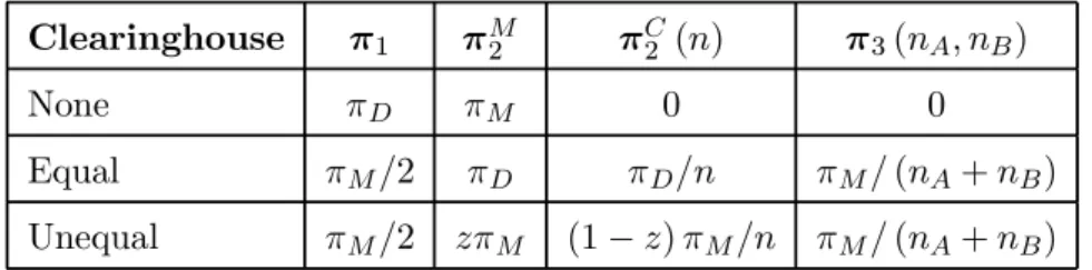
Clearinghouse π1 πM2 πC2 (n) π3(nA, nB)
None πD πM 0 0
Equal πM/2 πD πD/n πM/(nA+nB)
Unequal πM/2 zπM (1−z)πM/n πM/(nA+nB)
Table 1: Equilibrium payoffs of successful inventors under different types of clearinghouse and different outcomes of the innovation process.
If case 2 arises, the successful inventors of the competitive component will all join either type of clearinghouse, as explained above. If the competitive
component has n inventors, the inventor of the monopoly component will
join an equal clearinghouse if πM/(n+ 1) ≥ πD and will join an unequal
clearinghouse if zπM ≥ πD. To distinguish equal and unequal
clearing-houses, we make the following assumption:
Assumption 2 A monopoly inventor of a component does not join an equal clearinghouse when there are n ≥2 inventors of the other component, but does join an unequal clearinghouse. That is, πM ≤3πD and z≥πD/πM.1
We can now summarise the equilibrium payoffs of successful inventors in stage 2, depending on which of the three cases above has arisen from
the innovation process. Let π1 be the royalties that a successful inventor
receives in case 1, let πM
2 be the royalties that the monopoly inventor
re-ceives in case 2, letπC
2 (n) be the royalties that a successful inventor of the
competitive component receives in case 2 when there are n ≥ 2 inventors
of that component, and let π3(nA, nB) be the royalties that a successful
inventor receives in case 3 when there are nA≥2 successful inventors of A
and nB ≥2 successful inventors of B.
Table 1 shows the values of these payoffs for different types of clear-inghouse, as determined by the equilibrium of stage 2 of the model. In comparison with no clearinghouse, an equal clearinghouse increases an in-ventor’s royalties if there are multiple inventors of the same component, or if there is only one inventor of both components. However, the clearinghouse
decreases royalties fromπM toπDwhen the inventor is the sole inventor of
1Such a value ofz achieves the clearinghouse’s objective of maximising the total roy-alties of its members, since it ensures that all inventors join and consequently the clear-inghouse royalties areπM.
a component but the other component is competitive. In this situation, the existence of the clearinghouse reduces competition among inventors of the competitive component, which benefits them but harms the sole inventor of the other component.
An unequal clearinghouse increases a successful inventor’s royalties com-pared to no clearinghouse unless the inventor is the sole inventor of one component while the other component is competitive. In this case the value
ofz is sufficient to induce the monopoly inventor to join the clearinghouse,
but she is still worse off compared to when no clearinghouse exists, because
the clearinghouse gives some fraction ofπM to the competitive inventors of
the other component. An unequal clearinghouse may also make successful inventors better or worse off compared to an equal clearinghouse. If, for example, A has a single inventor but B is competitive, the inventors of B
receive πD/nB under an equal clearinghouse, but (1−z)πM/nB under an
unequal clearinghouse. Since z ≥ πD/πM to attract the inventor of A to
join the unequal clearinghouse, this reduces the payoffs of the inventors of B relative to the equal clearinghouse.
Similarly, let W1,W2 and W3 be the equilibrium welfare levels attained
from licensing in cases 1, 2 and 3 respectively. Table 2 shows the welfare levels (ignoring R&D costs) that result under each type of clearinghouse in each of the three cases. Compared to no clearinghouse, an equal clearing-house improves welfare when both components have a single inventor (case 1), but reduces welfare in all other cases, as the clearinghouse allows multiple inventors of the same component to reduce competition among themselves.
An unequal clearinghouse with an appropriate value ofzalways attracts all
inventors to join, and thus always achieves the welfare levelWM. Compared
to no clearinghouse, this increases welfare when both components have a single inventor (case 1), but reduces welfare when both components have multiple inventors (case 3), and leaves welfare unchanged in case 2. In every case an unequal clearinghouse generates at least as much welfare as an equal clearinghouse, and outperforms it when one component has a single inventor and the other has multiple inventors (case 2).
Clearinghouse W1 W2 W3
None WD WM W0
Equal WM WD WM
Unequal WM WM WM
Table 2: Equilibrium welfare (ignoring investment costs) from licensing un-der different types of clearinghouse and different outcomes of the innovation process.
3
Effects of clearinghouses on ex ante expected
profits and welfare
In this section we examine and compare clearinghouses under two alternative models of the investment and innovation process in stage 1 of the game.
3.1 Investment model 1: All projects are equal
In this model, every research project costs c and has the same chance of
developing a component or developing nothing. Research firms and projects are exogenously specialised towards the development of A or B and a large
number of firms are capable of undertaking projects of each type. LetNA
and NB be the total number of projects undertaken to develop A and B
respectively. The success of any project is independent of that of any other
project. Given thatNi ≥1projects are undertaken for componenti=A, B,
the probability thatni≤Ni successfully develop the component is denoted
by P(ni, Ni), where
Ni
ni=0P(ni, Ni) = 1 and limNi→∞P(ni, Ni) = 0 for allni ∈ {0,1, ..., Ni}.
Since the components are identical, we consider symmetric situations
where NA = NB = N, thus 2N projects are undertaken in total. The
expected profit of a research firm given thatN research projects are
under-taken for each component is denoted π(N). The probability that there is
one successful inventor of each component (case 1) and a given research firm
is one of these is N1P(1, N)
2
. The probability that a research firm is the sole
inventor of their component while the other component hasn≥2inventors
(case 2, monopoly) is 1
NP(1, N)P(n, N). The probability that a research
firm is one ofn≥2inventors of their component while the other component
proba-bility that a research firm is one ofm≥2inventors of their component while
the other component has n ≥ 2 inventors (case 3) is mNP(m, N)P(n, N).
Considering all possibilities under which cases 1, 2 and 3 can occur, using the payoff definitions from Table 1, the expected profit of a research firm is
π(N) = 1 NP(1, N) 2 π1+N1P(1, N) N n=2 P(n, N)πM2 +nπ C 2 (n) + N m=2 N n=2 m NP(m, N)P(n, N)π3(m, n)−c. (1) LetπN C (N),πEC (N)and πU C
(N)be a research firm’s expected profit
under no clearinghouse, an equal clearinghouse and an unequal clearinghouse
respectively given thatN projects are undertaken for each component.
Re-call from Table 1 that the existence of a clearinghouse potentially involves both ex post gains and losses for research firms. The following proposition shows that, in terms of ex ante expected profits, the gains always outweigh
the losses, for any givenN.
Proposition 1 Given N, the expected profit of a research firm is highest with an unequal clearinghouse and lowest with no clearinghouse, that is,
πU C
(N)≥πEC
(N)≥πN C
(N) for all N ≥1.
Proof. Substituting payoffs from Table 1 into (1), πU C
(N) ≥ πEC (N)
if P(1, N)Nn=2P(n, N) [πM −2πD] ≥ 0, which is true by Assumption
1. Similarly, πU C (N) ≥πN C (N) is equivalent toP(1, N)21 2πM−πD + N m=2 N n=2 m
m+nP(m, N)P(n, N)πM ≥0, which is also true by
Assump-tion 1. Finally,πEC (N)≥πN C (N) iff(N)πM ≥g(N) 2πD where g(N) =P(1, N)2−2P(1, N) N n=2 P(n, N) and f(N) =g(N) + 2 N m=2 N n=2 m m+nP(m, N)P(n, N).
SinceπM ≥2πDandf(N)≥g(N), we haveπEC(N)≥πN C(N)iff(N)≥
0for all N ≥1. To show this is true, note that f(N)≥0is the same as
1−2 N n=2 R(n, N) + 2 N m=2 N n=2 m m+nR(m, N)R(n, N)≥0,
withR(n, N) =P(n, N)/P(1, N), and this last inequality can be rewritten
asNn=2R(n, N)−1
2
≥0, which is true.2
Since research firms are competitive, the equilibrium number of projects,
N∗
, satisfiesπ(N∗
) ≥ 0 and π(N∗
+ 1)< 0. In this model, either type of
clearinghouse always increases the ex ante profits of a research firm, and thus generates greater investment in R&D compared to no clearinghouse, for a given level of per-project costs.
Using the welfare definitions from Table 2, expected total welfare given
thatN research projects are undertaken for each component is
W(N) = P(1, N)2W1+ 2P(1, N) N n=2 P(n, N)W2 + N m=2 N n=2 P(m, N)P(n, N)W3−2Nc (2) LetWN C (N), WEC (N) and WU C
(N) be the total expected welfare with
no clearinghouse, an equal clearinghouse and an unequal clearinghouse re-spectively. The following proposition compares the expected welfare gains and losses from introducing a clearinghouse.
Proposition 2 GivenN, expected welfare with an unequal clearinghouse is always higher than that with an equal clearinghouse: WU C
(N)≥WEC (N)
for all N ≥1. In addition, expected welfare with no clearinghouse is high-est when N is sufficiently large but lowest when N is small: WU C
(N) ≥
WEC
(N)≥WN C
(N)for sufficiently smallN, andWN C
(N)≥WU C (N)≥
WEC
(N) for sufficiently large N. Proof. From Table 2 it is clear thatWU C
(N)≥WEC
(N)sinceWM ≥WD.
From Table 2 and (2),WU C
(N)≥WN C (N) if P(1, N)2[WM −WD]≥ N m=2 N n=2 P(m, N)P(n, N) [W0−WM].
SinceNn=2P(n, N) = 1−P(0, N)−P(1, N), this can be rewritten as
1−P(0, N)−P(1, N) P(1, N) 2 ≤ WM −WD W0−WM .
2This follows from the fact that given some numbers
x1, ..., xN, 2 N i=1 N j=1 i i+jxixj= N i=1 N j=1 xixj= N i=1 xi 2 .
The right-hand side of this inequality is positive since W0 ≥ WM ≥ WD.
If N = 1 the left-hand side equals zero since P(0,1) +P(1,1) = 1, so
WU C
(1)> WN C
(1). At higher values of N, the left-hand side eventually
becomes arbitrarily large, since limN→∞P(n, N) = 0 for all n, thus for
sufficiently largeN this inequality does not hold andWU C
(N)< WN C (N). Finally, WEC (N)≥WN C (N) if 1−2 N n=2 P(n, N) P(1, N) [WM −WD]≥ N m=2 N n=2 P(m, N) P(1, N) P(n, N) P(1, N) [W0−WM] which can be rewritten as
P(1, N) [2P(0, N) + 3P(1, N)−2] [1−P(0, N)−P(1, N)]2 ≥
W0−WM
WM −WD.
The right-hand side is positive while the left-hand side is arbitrarily large
atN = 1and converges to zero as N increases. ThusWEC
(1)> WN C (1),
and WEC(N)≤WN C(N) for sufficiently large N.
Intuitively, an unequal clearinghouse always generates more welfare than an equal clearinghouse because, given that both components are invented,
it guarantees that the welfare level with a single licensor,WM, is achieved,
while the equal clearinghouse only achievesWD≤WM in the case when one
component has a single inventor while the other component has multiple inventors. However, no clearinghouse outperforms both types of
clearing-house when N is large. This is because when N is large, the most likely
outcome is that both components have multiple inventors (case 3). In this case, with no clearinghouse, competition among inventors drives royalties
for both components to zero, and the highest possible welfare level, W0, is
achieved from licensing. Similarly, no clearinghouse generates low welfare
levels relative to both types of clearinghouse whenN is low, because then
it is more likely that both components have a single licensor and thus joint
licensing through a clearinghouse achievesWM instead ofWD.
Propositions 1 and 2 also imply that there is a potential tradeoff in terms of the equilibrium effects of a clearinghouse on expected welfare. For any
given level of investment in R&D (givenN), introducing some sort of
clear-inghouse may or may not raise expected welfare. However, even if welfare
increases givenN, it is not guaranteed to increase once the increase in
invest-ment is taken into account, since R&D is costly. Without making additional assumptions it is impossible to solve the zero-profit condition on (1) to de-termine the equilibrium R&D investment and perform comparative statics
analysis between the different clearinghouse regimes. We therefore use a numerical simulation model in section 4 to examine this tradeoff further.
There may also be a conflict between the incentives of existing intel-lectual property owners and research firms who have not yet invested, in terms of their willingness to use and support a clearinghouse. For example, Table 1 shows that if case 2 arises, the monopoly inventor is made worse off by the existence of either type of clearinghouse relative to when there is no clearinghouse. Sole successful inventors of an essential component for a downstream innovation may thus be reluctant to use a clearinghouse if it means that they have to share some royalties with competitive inventors of
another component. On the other hand, Proposition 1 showed that the ex
anteexpected profit of a research firm is always increased by the creation of
a clearinghouse. Thus innovators who have not yet invested are more likely to support the creation of the clearinghouse, even if, ex post, there is some chance that they will have a monopoly over their component.
3.2 Investment model 2: Component A is unique
In this version of the model, a single research firm (‘firm A’) has the unique ability to develop component A. We assume its success is deterministic,
and it can develop A for certain if it invests cA. As before, there are also
competitive research firms that each can undertake one research project to
try to develop B at a cost of cB. Given that N projects are undertaken
by these component B firms, the probability that n of them are successful
is P(n, N). We let πA(N) denote firm A’s expected profit given that it
invests and given that N projects invest in B, and let πB(N) denote the
expected profit of an individual project aimed at developing B given that firm A invests.
Of licensing cases 1, 2 and 3 considered earlier, only 1 and 2 are possible in this model. Given that firm A invests, the probability that there is a single
inventor of both components (case 1) isP(1, N)and the probability that A
has a single inventor while B has multiple inventors (case 2) isP(n, N) for
n≥2. Thus we have πA(N) =P(1, N)π1+ N n=2 P(n, N)πM2 −cA. (3)
Proposition 3 Given N, Firm A is always better off under an unequal clearinghouse compared to an equal clearinghouse when Assumption 2 holds. In addition, firm A’s expected profit is highest with no clearinghouse for relatively high values of N, but is highest with an unequal clearinghouse for relatively low values of N. That is, πN C
A (N) ≥ π
U C
A (N) ≥ π
EC
A (N) for
sufficiently high N and πU C
A (N)≥π
EC
A (N)≥π
N C
A (N) for sufficiently low
N.
Proof. From Table 1 and (3),πU C
A (N)≥π
EC
A (N) if
[1−P(0, N)−P(1, N)] (zπM −πD)≥0
which is true for all N under Assumption 2. Similarly πU CA (N)≥π
N C A (N) if P(1, N) 1−P(0, N)−P(1, N) ≥ 2 (1−z)πM πM −2πD .
The right-hand side of this expression is positive by assumption. The
left-hand side is arbitrarily large when N = 1, so πU C
A (1) ≥ π
N C
A (1). As N
increases, the left-hand side converges to zero, since limN→∞P(n, N) =
0 for all n, thus for sufficiently large N, πU C
A (N) < π N C A (N). Finally, πEC A (N)≥π N C A (N) if P(1, N) 1−P(0, N)−P(1, N) ≥ πM −πD 1 2πM −πD .
Again the right-hand side is positive and this expression holds at N = 1,
but the left-hand side converges to zero asN increases.
Firm A always prefers an unequal clearinghouse to an equal one provided
that the unequal clearinghouse sets z high enough so that it induces firm
A to join ex post. In comparison to no clearinghouse, firm A prefers a
clearinghouse only when N is small and the probability that component
B has a single inventor is relatively large. In that case, firm A benefits from the existence of a clearinghouse because joint licensing with a single inventor of B increases A’s profits. However, if B has multiple inventors, competition among them drives the royalty for B to zero, and firm A is able to appropriate all of the monopoly profits from licensing when there is no clearinghouse. If an equal clearinghouse exists, in such a situation the inventors of B will license jointly, which hurts firm A, while if an unequal clearinghouse exists, firm A also joins, but has to share some royalties with
the inventors of B. In either case, firm A is worse off compared to when no clearinghouse exits.
The expected profit of a research firm that develops B is
πB(N) = 1 NP(1, N)π1+ N n=2 n NP(n, N)π C 2 (n)−cB. (4)
Proposition 4 For any given N, a research firm that invests in compo-nent B is always better off under either an equal or unequal clearinghouse compared to no clearinghouse. Such a firm is better off under an unequal clearinghouse compared to an equal clearinghouse ifz≤1−πD/πM.
Proof. From Table 1 and (4), it is straightforward to verify that the
assumption that πM ≥ 2πD guarantees that πECB (N) ≥ πN CB (N) and
πU C
B (N) ≥ π
N C
B (N) for all N ≥ 1. We also have π
U C B (N) ≥ π EC B (N) if 1 N [1−P(0, N)−P(1, N)] [(1−z)πM −πD]≥0
which is true provided thatz≤1−πD/πM.
Having either type of clearinghouse never makes a component B research firm worse off because the firm always gets a strictly higher ex post payoff whatever the outcome of the random innovation process compared to when there is no clearinghouse in this model, as shown in Table 1. Whether an unequal clearinghouse is better than an equal clearinghouse for these firms depends on the fraction of revenues that the unequal clearinghouse gives
to firm A. Both types of clearinghouse give the same payoff, πM/2, to a
component B inventor when there is a single successful inventor of that component. When there are multiple successful inventors of B, an equal
clearinghouse does not induce firm A to join, so an inventor of B getsπD/n.
With an unequal clearinghouse, firm A joins and the clearinghouse revenues
rise to πM, but a fraction z is given to firm A to induce it to join. Thus
component B inventors are only better off relative to an equal clearinghouse
if z is not too large. Note that there is always some range of z that both
induces firm A to join an unequal clearinghouse and makes component B
inventors better off compared to an equal clearinghouse. This requiresz ∈
[πD/πM,1−πD/πM], which is always feasible sinceπD/πM ≤ 12.
Combining Propositions 3 and 4, the existence of a clearinghouse in-creases the incentive of component B firms to invest in R&D, but may
increase or decrease firm A’s incentive to invest. In addition, if the in-troduction of a clearinghouse increases investment by component B firms,
this in turn may increase or decrease firm A’sex ante profit. Overall,
intro-ducing a clearinghouse will increase investment in component B, but has an ambiguous effect on firm A’s incentive to invest.
As in the first investment model, there may also be a conflict between existing and potential innovators. For example, if firm A has already in-vested, it will be opposed to a clearinghouse if there are multiple inventors of component B. This model also generates a conflict between firm A and component B firms. Under an unequal clearinghouse, if firm A has already
invested it will want z to be as high as possible. However, having no
clear-inghouse or a high value of z reduces the expected profits of a component
B research firm. On the other hand, if investment has not yet taken place, ex ante firm A may be willing to sacrifice some of its ex post profits, by
supporting a clearinghouse or a lower value ofz, to give greater incentive to
the component B firms to invest, since A cannot earn any revenues unless B is also invented. We examine these tradeoffs further numerically in the next section.
The expected welfare given that firm A invests and N ≥1 other firms
invest is W(N) =P(1, N)W1+ N n=2 P(n, N)W2−cA−NcB. (5)
Proposition 5 GivenN, expected welfare is always highest with an unequal clearinghouse, under Assumption 2. An equal clearinghouse generates higher welfare compared to no clearinghouse only for sufficiently low N. That is,
WU C
(N)≥WEC
(N)≥WN C
(N) for sufficiently lowN, and WU C (N)≥
WN C
(N)≥WEC
(N) for high N.
Proof. From Table 2 and (5), it is straightforward to show thatWM ≥WD
implies WU C (N) ≥ WEC (N) and WU C (N) ≥ WN C (N) for all N ≥ 1. Similarly,WEC (N)≥WN C (N) if [2P(1, N) +P(0, N)−1] [WM −WD]≥0.
This is true atN = 1sinceP(1,1) +P(0,1) = 1and WM ≥WD. However
the first bracket converges to −1 as N becomes large, thus WEC
(N) < WN C
In this model the unequal clearinghouse always does best in terms of expected welfare. This is because with a unique inventor for component A, a situation in which there are multiple inventors of both components
never arises, and the welfare level W0 is never achieved. Thus since the
unequal clearinghouse guarantees the welfare level WM, provided that z
is high enough that firm A joins, it always performs better than either no clearinghouse or an equal clearinghouse. On the other hand, an equal
clearinghouse only outperforms no clearinghouse if N is low so that the
chance that component B has a single inventor is relatively high. WhenN
is large, it is relatively likely that competition among inventors of B will
drive the royalty for that component to zero, resulting in welfare levelWM
with no clearinghouse. However, an equal clearinghouse permits multiple
inventors of B to reduce competition, resulting in welfare ofWD.
Finally, as in model 1, the ranking of expected welfare in Proposition 5 takes the level of investment in R&D as given. While an unequal
clearing-house always results in the highest expected welfare level givenN, once the
change in investment induced by the clearinghouse is taken into account, a clearinghouse may either increase or decrease ex ante expected welfare.
3.3 Summary
The above analysis shows that clearinghouses have some different effects in the two different investment models. Here we summarise the results we have obtained so far and compare clearinghouses versus no clearinghouse in terms of ex ante and ex post profits and welfare.
Ex ante profit: In model 1, introducing a clearinghouse increases ex
ante profit for all N, while in model 2 ex ante profit always increases for
component B firms, but only increases for firm A whenN is relatively low.
Ex post profit: In both models, introducing a clearinghouse increases the ex post profit of inventors of a component that has multiple inventors. It also increases inventors’ profits when both components have a single inventor. Thus, ex post, component B inventors are always better off from introducing a clearinghouse in model 2. However, a clearinghouse reduces the ex post profit of the sole inventor of one component when the other component is competitive. Thus any research firm has a chance of being made worse off in model 1, and firm A may be made worse off in model 2 if B is competitive.
increases welfare relative to no clearinghouse whenN is low, but decreases
welfare whenN is high. In model 2, the same is true for an equal
clearing-house, but an unequal clearinghouse always increases ex ante welfare relative to no clearinghouse, provided that firm A invests.
Ex post welfare: Either type of clearinghouse increases ex post welfare in both models when both components have a single inventor. When one component has a single inventor and the other component has multiple in-ventors, under both models an equal clearinghouse decreases ex post welfare while an unequal clearinghouse leaves welfare unchanged. If both compo-nents have multiple inventors, which only arises in model 1, both types of clearinghouse reduce ex post welfare.
4
Simulation analysis
In this section we use numerical simulations of our two investment models to investigate further the tradeoffs between welfare and incentives to invest that were identified above. For the simulation we assume that total demand for
licenses from both components is linear and is given byQ= 100−ρwhereQ
is the number of licenses sold andρis the total per-unit royalty for licensing
both A and B. Under this assumption, the royalty revenues of a licensor
setting a royalty ofri isRi = (100−ρ)ri whereρ=ri, and total welfare
generated by licensing is W = 50 (1−ρ) (1 +ρ). When there is a single
licensor, ρ is chosen to maximise (100−ρ)ρ, which gives ρM = 12. Under
duopoly, it is straightforward to show that the noncooperative equilibrium
royalties are ρD =
2
3. These give the parameter values shown in Table 3.
It is clear that these values satisfy Assumption 1. To satisfy Assumption 2,
the unequal clearinghouse must setz∈4
9,1
.
We also assume that the random investment processes are binomial, with
the probability of success of any given project given by σ, thus
Pr (n, N) =σn(1−σ)N−n N!
n! (N −n)!.
The exogenous parameters of the simulation model are therefore the success
probability σ, the unequal clearinghouse parameter z, and the investment
costs c (in model 1) and cA and cB (in model 2). Simulations were
pro-grammed in R 2.6.0 for Windows, and source codes are available from the
Parameter πM πD W0 WM WD
Value 1004 1009 50 75 2
250 9
Table 3: Model parameters for linear demand for licensing, where Q =
100−ρwith ρthe total per-unit royalty.
4.1 Model 1 simulations
The key question from model 1 is how introducing either type of clearing-house affects equilibrium investment in the two components and hence the expected equilibrium welfare level. We examined this by using a simulation
that iterates over a grid of values ofc and σ. For each pair of parameters
the equilibrium investment level is found by evaluating (1) and using a
nu-merical search algorithm to find the highest level of N at whichπ(N) ≥0
and π(N+ 1) < 0. With binomial success probabilities, π(N) eventually
approaches−casN becomes large, since the probability that any individual
project is successful tends to zero. Thus provided thatπ(N) >0 for some
relatively low values of N, an equilibrium with investment in both
compo-nents exists. Otherwise, we recorded the equilibrium asN = 0, representing
no investment.
For each combination of cand σ, this procedure was repeated assuming
no clearinghouse, an equal clearinghouse and an unequal clearinghouse, and
the equilibrium level of investment was recorded in each case.3 Under each
type of clearinghouse, the welfare level at the equilibrium investment level
was calculated by evaluating (2). Thus for each combination ofcandσ, we
record six values: the equilibrium investment level and the equilibrium wel-fare level under no clearinghouse and each of the two types of clearinghouse.
We allowedcto vary between0.1and10in increments of0.01andσ to vary
between0.05 and 0.95in increments of 0.001, thus we conducted a total of
892,891simulations for model 1.
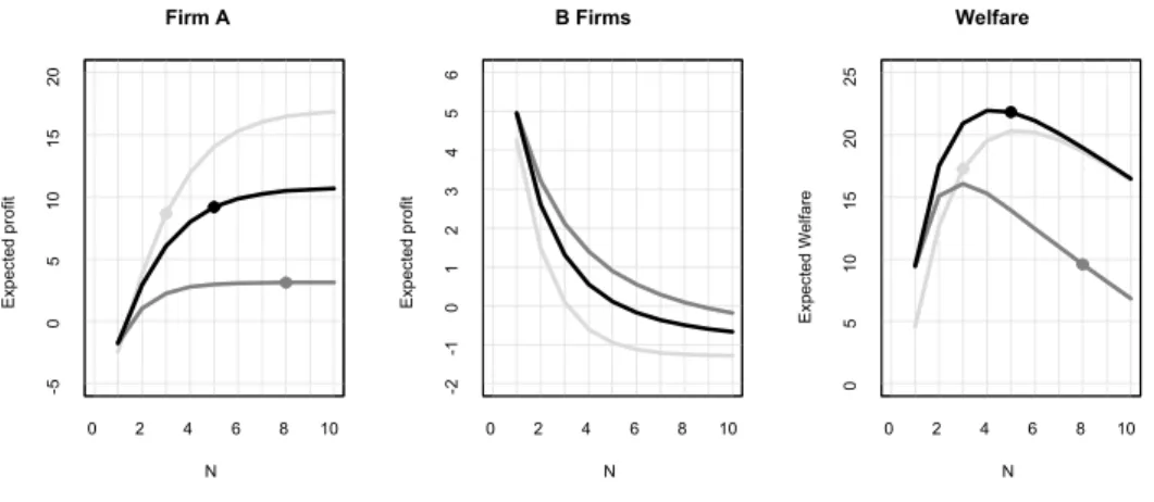
Figure 1 illustrates a single example simulation of model 1, for the
pa-rameter values shown in Table 3, and assuming c = 2.5 and σ = 0.7. The
left panel shows the expected profit of an individual research firm under each type of clearinghouse, as a function of the number of projects that are undertaken for each component. As in Proposition 1, introducing a
clear-3Note that in model 1 with an unequal clearinghouse, it is straightforward to show that expected profits are independent ofz, by substituting payoff from Table (1) into (1).
Profit N E x p e c te d p ro fi t 0 1 2 3 4 5 6 7 8 9 10 -3 -2 -1 0 1 2 3 4 None Equal Unequal Welfare N E x p e c te d w e lf a re 0 1 2 3 4 5 6 7 8 9 10 -1 0 0 1 0 2 0 3 0
Figure 1: Illustration of a single simulation of model 1, for c = 2.5 and
σ = 0.7. The left plot shows expected profits of a research firm given
that N projects are undertaken for each component, under each type of
clearinghouse. The right plot shows expected welfare as a function of N.
The large dots are the equilibrium welfare levels.
inghouse increases expected profit for all N. In this particular case, there
is very little difference in terms of profit between an equal and an unequal clearinghouse. Under no clearinghouse, the equilibrium investment level is
N = 2, while under an equal or unequal clearinghouse it is N = 4. The
right panel plots expected welfare as a function of N under each type of
clearinghouse, and the large dots show the equilibrium welfare levels.
In this case, the increase in investment from N = 2 to N = 4 would
increase expected equilibrium welfare if the clearinghouse had no effect on ex post royalties. As Figure 1 shows, equilibrium welfare on the no
clearing-house curve is higher atN = 4compared toN = 2because the probabilities
that both components are successfully developed and both components have competitive inventors are higher, and these gains outweigh the costs of the additional research projects. However, once changes in ex post licensing are taken into account, introducing a clearinghouse reduces equilibrium welfare for these parameter values.
Repeating this process for all combinations of c and σ within the given
range allows us evaluate each type of clearinghouse in terms of the equi-librium welfare level as a function of the parameters. Figure 2 shows the results of this analysis by graphing the regions where equilibrium welfare is highest with no clearinghouse, an equal clearinghouse, or an unequal
clear-Figure 2: Parameter regions in which equilibrium expected welfare in model 1 is highest under each type of clearinghouse.
inghouse for different combinations ofcandσ. In general, no clearinghouse
performs best when the cost per project is relatively low, or the probability of success of an individual project is relatively high. When the per-project cost increases, everything else equal, investment falls under all clearinghouse types. At sufficiently high cost levels, having a clearinghouse may increase welfare, as it increases the probability that both components are successfully invented and the product can be produced. When the probability of success increases, everything else equal, it becomes more likely that both compo-nents will have competitive inventors for a given investment level, and in this case the ex post welfare is highest with no clearinghouse. If both the project cost and probability of success are relatively high, the welfare level under an equal and unequal clearinghouse is the same, and this dominates no clearinghouse. In these cases, costs are so high that no investment oc-curs with no clearinghouse, while exactly one project is conducted for each component under both types of clearinghouse, in which case the equal and unequal clearinghouses produce the same welfare level.
Figure 3 further illustrates the complex structure observed at the bound-aries in Figure 2 by showing the equilibrium investment level and associated
Equilibrium Investment c N o . p ro je c ts 0 2 4 6 8 10 0 4 8 1 2 1 6 2 0 2 4 2 8 None Unequal Equilibrium Welfare c E x p e c te d w e lf a re 0 2 4 6 8 10 0 1 0 2 0 3 0 4 0
Figure 3: Equilibrium investment and welfare in model 1 as a function of the
per-project costc, assuming σ= 0.57, for no clearinghouse and an unequal
clearinghouse.
expected welfare as functions ofc, holdingσ fixed at 0.57, under no
clear-inghouse and an unequal clearclear-inghouse. Provided that c is not too high,
investment occurs under both no clearinghouse and an unequal clearing-house, and the existence of a clearinghouse generally raises the investment
level for givenc. The higher level of investment plus the fact that the
clear-inghouse results in higher royalties in many cases generally serves to reduce expected welfare. However, if investment did not occur with no clearing-house but does occur with a clearingclearing-house, then welfare is higher with the
clearinghouse. In addition, in some cases (for c between around 3 to 3.5),
investment levels both with and without a clearinghouse are not very high
(around2or3projects). In this case, it is relatively unlikely that either
com-ponent will have multiple inventors, and thus the expected welfare benefits of having a clearinghouse outweigh any expected losses.
4.2 Model 2 simulations
Simulations of model 2 were conducted in a similar manner as for model 1. In model 2, for there to be some probability of production, firm A must invest and at least one component B firm must invest. Using (3) and (4)
we search for the largest value of N where πA(N) ≥ 0, πB(N) ≥ 0 and
πB(N+ 1)<0. As in model 1, the expected profit of a component B firm
investment occurs if πB(N) ≥0 and πA(N) ≥ 0 for some relatively small
N. As well as the linear demand royalties and welfare from Table 3, the
other parameters in model 2 are cA, cB,σ and z. In general we normalise
cA and allow cB to vary. Unlike in model 1, in model 2 the asymmetry
between the component A and B research firms means that z has an effect
on the expected profits of both firm A and the component B research firms. Figure 4 illustrates a single simulation of model 2, for some particular
parameter values. With no clearinghouse the equilibrium is N = 3, with
an equal clearinghouse it is N = 8 and with an unequal clearinghouse it is
N = 5. In this case,z >1−πD/πM, so following proposition 4, the expected
profits (and hence investment level) of component B firms is highest under an equal clearinghouse, followed by an unequal clearinghouse and then no clearinghouse. In all of these three cases, the expected profit of firm A is positive, so it invests. For these parameter values, expected equilibrium welfare is highest with an unequal clearinghouse. As in proposition 5, for any
given N, an unequal clearinghouse generates the highest expected welfare
level in model 2. For the parameter values shown in Figure 4, the welfare benefits of having an unequal clearinghouse compared to no clearinghouse plus the increased probability that component B is successfully developed more than offset the costs of the additional investment in component B that is induced. However, an equal clearinghouse would reduce expected welfare compared to no clearinghouse as it stimulates too much investment in component B.
As noted above, the value of z under an unequal clearinghouse is not
neutral in this model. Given any N ≥2, a higher value of z increases the
expected profit of firm A and reduces the expected profit of a component
B research firm under an unequal clearinghouse. Thus higherz will reduce
investment in component B, but make it more likely that firm A will find in-vesting profitable, everything else equal. Figure 5 illustrates this tradeoff by showing firm A’s expected profit and expected equilibrium welfare as
func-tions ofz, for some specific values ofcA,cB and σ. To generate this figure,
for each value of z in the feasible range, the equilibrium investment levels
under an unequal clearinghouse were calculated in the manner described above, and the corresponding expected profits of firm A and expected wel-fare were calculated. The discrete steps observed in the results correspond to different discrete levels of equilibrium investment in component B.
Firm A N E x p e c te d p ro fi t 0 2 4 6 8 10 -5 0 5 1 0 1 5 2 0 B Firms N E x p e c te d p ro fi t 0 2 4 6 8 10 -2 -1 0 1 2 3 4 5 6 Welfare N E x p e c te d W e lf a re 0 2 4 6 8 10 0 5 1 0 1 5 2 0 2 5
Figure 4: Illustration of a single simulation of model 2, forcA= 8,cB = 1.3,
σ = 0.5 and z = 0.75. The left plot shows expected profits of firm A
given thatN projects are undertaken for component B, under each type of
clearinghouse. The middle plot shows the expected profit of a component
B research firm. The right plot shows expected welfare as a function of N
and the large dots are the equilibrium welfare levels.
When the probability of success for component B firms (σ) is low, Figure
5 shows that expected profits and welfare generally decline as z increases.
With lowσ, equilibrium investment in component B is low, while equilibrium
welfare is increasing inN provided thatcB is not too large, since additional
investment would raise the probability that component B is invented. In this
case, increasingz reduces investment in component B and reduces expected
welfare. Reduced investment in component B also negatively affects firm A in this case as it can only earn profits if component B is also invented. Thus
when σ is low, ex ante firm A prefers a low value of z as this stimulates
investment in component B, even though it may reduce firm A’s ex post licensing profits.
At higher values of σ, Figure 5 shows that equilibrium expected profits
of firm A and welfare may be increasing and then decreasing in z. Again
increasingzreduces investment in component B under an unequal
clearing-house. However, this may increase welfare ifσ is sufficiently high, since the
cost savings from reduced investment can outweigh the reduced probability
that component B is invented. Indeed, ifσ is very high then expected
sigma = 0.25 z E x p e c te d P ro fi t, W e lf a re 0.4 0.6 0.8 1.0 0 5 1 0 1 5 2 0 2 5 3 0 sigma = 0.5 z E x p e c te d P ro fi t, W e lf a re 0.4 0.6 0.8 1.0 0 5 1 0 1 5 2 0 2 5 3 0 sigma = 0.75 z E x p e c te d P ro fi t, W e lf a re 0.4 0.6 0.8 1.0 0 5 1 0 1 5 2 0 2 5 3 0 Firm A profit Welfare
Figure 5: Firm A’s expected equilibrium profit and expected equilibrium
welfare under an unequal clearinghouse as a function of z, for cA = 5 and
cB= 3.
case, investment in B is minimal since investors only get a return if they are the sole successful investor, but this does not have a large adverse effect on firm A’s expected profits or expected welfare.
Figure 6 shows parameter combinations of cB and σ where each type
of clearinghouse performs best in terms of ex ante expected welfare, for
different values ofz, holdingcAconstant. Again we simulated the model for
all combinations ofcBbetween0.1and10(in increments of0.01) and values
ofσbetween0.05and0.95(in increments of0.001), for three different values
in the feasible range of z. In total, 2,678,673simulations of model 2 were
Figure 6: Parameter regions in which equilibrium expected welfare in model
performed. In each case, the equilibrium under each type of clearinghouse was recorded and the corresponding equilibrium expected welfare level was
calculated. As in model 1, given z, clearinghouses generally perform best
when the cost of R&D is relatively high or the probability of success is relatively low.
In addition, comparing the results in Figure 6 for different values of z
shows that as z increases, the range of parameters where no clearinghouse
performs best shrinks and the range where an unequal clearinghouse
per-forms best expands. This is because as z increases, the ex post payoffs to
firms under an unequal clearinghouse and no clearinghouse become similar, except in the case where both components have a single inventor, as can be seen from Table 1. Thus the level of investment achieved by an unequal
clearinghouse is similar to that with no clearinghouse when z is large, but
the clearinghouse increases welfare as it results in more efficient licensing when both components have a single inventor. Nevertheless, this does not
necessarily mean thatz= 1orzclose to1is the socially optimal value ofz.
For some parameter values, increasingzdoes make an unequal clearinghouse
perform better than no clearinghouse, but as shown in Figure 5 once effects on the level of investment are taken into account, the welfare-maximising
value of zcan be anywhere within the feasible range.
Figure 6 also shows that aszincreases the range of parameters where an
equal clearinghouse outperforms an unequal clearinghouse increases. The ex post welfare under an equal clearinghouse may be less than that of an unequal clearinghouse, as the equal clearinghouse does not result in the participation of firm A when component B has multiple inventors. However, the equal clearinghouse gives stronger incentives to component B firms to
invest compared to an unequal clearinghouse with a high value of z, which
may be preferable from a welfare point of view.
5
Conclusion
Our analysis has shown that clearinghouses can have both positive and neg-ative effects on ex ante and ex post profits and welfare from licensing in-novations. Taking a long-run perspective, the ex ante effects on expected profits and welfare are arguably the most important. In this case we showed that clearinghouses generally increase expected profits from licensing. An
exception is when there is a unique potential inventor for one component (our model 2), in which case a clearinghouse may reduce that inventor’s expected profits when investment in the other component is relatively high. Aside from this exception, clearinghouses generally increase incentives to invest in R&D. However, as we showed, this increase in investment does not always increase ex ante expected welfare, if the benefits in terms of the increased probability that all necessary components are developed does not outweigh the additional cost of the R&D investment and any anticompetitive effects of the clearinghouse.
The possibility that a clearinghouse reduces welfare is particularly acute in the case where royalties are distributed equally among members. If a clearinghouse does not have the ability to differentiate royalty payments to inventors whose innovations have no substitutes versus payments to those who do have competitive substitutes, the clearinghouse increases expected profits from R&D but is likely to reduce expected welfare. Therefore, we reach the policy conclusion that clearinghouses should be given flexibility in their royalty distribution scheme. Our analysis also showed that the optimal level of asymmetry of royalty payments by a clearinghouse to inventions with no substitutes versus those with substitutes varies depending on parameters such as the costs of R&D and the probability of success. If a clearinghouse spans multiple industries, for example, it may therefore be appropriate for it to use different royalty distribution arrangements in different cases, de-pending on industry characteristics.
Finally, our analysis highlighted some potential conflicts among different types of inventors in terms of their support for a clearinghouse. Clearing-houses are most likely to be supported by successful inventors of competitive innovations. However, their support should be viewed with some scepticism, as it is essentially a collusive device for them. On the other hand, symmet-ric inventors who have not yet invested and who all have an equal chance of being successful are also likely to support a clearinghouse, but this may enhance both profits and welfare if it does not induce excessive investment. Opposition to a clearinghouse is likely to come from successful inventors of a component that does not have any substitutes, or inventors who have not yet invested but have the unique ability to develop a component. In either case, an unequal royalty distribution scheme is necessary to earn their support.
References
[1] Aoki, R. & S. Nagaoka (2005). Coalition formation for a consortium standard through a standard body and a patent pool: Theory and ev-idence from MPEG2, DVD and 3G. Institute of Innovation Research,
Hitotsubashi University, Working Paper WP#05-01.
[2] Aoki, R. & A. Schiff (2008). Promoting access to intellectual property:
Patent pools, copyright collectives and clearinghouses. R&D
Manage-ment, forthcoming.
[3] Buchanan, J. & Y. Yoon (2000). Symmetric tragedies: Commons and
anticommons.Journal of Law and Economics,43: 1-13.
[4] Heller, M. & R. Eisenberg (1998). Can patents deter innovation? The
anticommons in biomedical research. Science,280: 698-701.
[5] OECD (2002). Genetic Inventions, Intellectual Property Rights
and Licensing Practices: Evidence and Policies. Downloaded from www.oecd.org/dataoecd/42/21/2491084.pdf.
[6] Shapiro, C. (2001). Navigating the patent thicket: Cross licenses, patent pools and standard setting. In Jaffe, E., Lerner, J. & Stern, S., eds,
Innovation Policy and the Economy, Volume I. MIT Press: Cambridge.
[7] Van Overwalle, G., E. van Zimmeren, B. Verbeure, G. Matthijs (2006).
Models for facilitating access to patents on genetic innovations. Nature
Reviews Genetics,7: 143-154.
[8] van Zimmeren, E., B. Verbeure, G. Matthijs & G. Van Overwalle (2006). A clearing house for diagnostic testing: The solution to ensure access to
and use of patented genetic innovations? Bulletin of the World Health