Do Foreign Direct Investment and Trade
Openness Accelerate Economic Growth?
The Honors Program
Senior Capstone Project
Student’s Name: Donna Chan Wah Hak
Faculty Sponsor: Dr. Edinaldo Tebaldi
April, 2011
Abstract ... 2
Introduction ... 3
Literature Review ... 6
Foreign Direct Investments and Economic Growth ... 6
Trade Openness and Economic Growth ... 9
Conditional Convergence and Economic Growth ... 13
Methodology and Empirical Models ... 18
Dataset and Variables ... 23
Discussion of Results ... 26
Conclusion ... 37
Appendices ... 40
Appendix A – Regression Analysis for Model 1 ... 41
Appendix B – Regression Analysis for Model 2 ... 42
Appendix C – List of Countries ... 43
ACKNOWLEDGEMENTS
I would like to express my deep and sincere gratitude to my advisor, Professor Edinaldo Tebaldi, for his guidance, constructive comments, and support throughout this work. I wish to express my warm and sincere thanks to Alison MacLeod for spending hours reviewing and proofreading this research paper.
I would like to thank Professor Mohan, my editorial reviewer, for his feedback. Many thanks also go to Professor Sousa, and the Honors Program.
I wish to thank my family for providing a loving environment for me. Jason, Laura, and Kelly, thank you for being the best siblings. I can always count on you to cheer me up. My grandparents, aunts, uncles, and cousins, thank you for believing in me.
Lastly, and most importantly, I wish to thank my parents, Ben and Helene Chan Wah Hak. They have provided a constant source of love and support – emotional, moral, and financial. They bore me, raised me, supported me, taught me, and loved me.
I would like to dedicate my Honors thesis to my aunt, Matante Ah Vee, and grandmother, Popo Colonne, who both recently passed away.
ABSTRACT
This research investigates the impact of trade openness and foreign direct investment (FDI) on economic growth. Using a framework proposed by Barro (1991), panel data regression
analysis is performed on 5-year time periods between 1985 and 2005. A sample of 89 countries is analyzed using data collected from the World Development Indicators (WDI), Penn World Table, Barro and Lee (2010), and Polity IV Project datasets. The empirical analysis shows that conditional convergence occurs among the countries in the sample and that FDI net inflows per worker slightly increases the speed of conditional convergence. This study also finds evidence that FDI has significant effects on economic growth. While
international trade does not significantly influence economic growth, human capital does. The presence of a democratic government also brings positive effects to growth in real GDP per capita.
INTRODUCTION
International trade and capital mobility play important roles in determining a country’s economic growth, represented by productivity and output levels. Openness to the world economy leads to industrialization, job creation, income growth, and development in the home country. The rationale is that trade increases domestic and international competition, which in turn, influences an economy’s productivity. Through exports, a country is able to experience a higher demand for its goods and services, increasing the output levels. Importing goods and services from foreign countries is said to enhance efficiency and productivity of domestic firms, leading to economic growth. Because developing nations may lack the knowledge and technology to utilize their resources efficiently and effectively, international trade and foreign investments may serve as substitutes for such, exposing these economies to new technologies and intellectual capital, which will then lead to economic growth.
Moreover, foreign direct investments (FDI) and international trade may influence the rate of economic growth such that conditional convergence occurs. Conditional convergence is the process that allows countries to reach their steady state. The technical diffusion from advanced economies to low income or developing nations can partially explain conditional convergence. The growth rate of a developing nation is predicted to be higher as it adopts and implements new technologies from advanced nations.
Economists such as Adam Smith, believe trade to be beneficial because countries highly involved in trading tend to have higher economic growth. In Wealth of Nations, Smith (1776) discusses the advantages of unregulated trade, stating a country shall produce the goods at which it is most efficient. Ricardo (1817) extends the free trade argument, suggesting that there is mutual benefit from trade because of comparative advantage. Any nation shall be able to achieve cost advantages in one way or another, thereby benefiting from international trade. According to Weil (2008), the average growth rate of GDP per capita over the period 1965-2000 in a closed economy was around 1.5%, and 3% for open nations. International trade and FDI are expected to enhance a country’s capital flows, and thus impact output growth.
Developed countries, having the necessary capital and technology, invest in developing countries in order to exploit their resources. In 2009, high income countries experienced a net
FDI outflow of $368.25 trillion (current US$) while low and middle income countries had $196.78 trillion (current US$) worth of net FDI flow (World Development Indicator, WDI). FDI is thus likely to flow from developed countries to developing countries. International trade, a key component of GDP, has also increased over time. In 2007, low and middle income countries depended more on international trade, as trade accounted for 62% of their GDP, an increase from the 38% in 1990 (WDI). Since there have been extensive trade and foreign investments, it is important to determine if that boom in investment and trade was beneficial to the economic growth, particularly of developing countries, and if these factors led to conditional income convergence. Conditional income convergence is represented by a higher percentage of GDP growth for low and (lower) middle income countries towards their steady states compared to high income countries. In 2005, high income countries’ GDP grew at a rate of 2.7% while low and middle income countries grew at a rate of 7.2% (WDI). Since low and middle income countries are further away from their steady states, they need to grow faster to reach these states.
Empirical efforts to link international trade and FDI to GDP have provided mixed results. Blomstrom et al (1994) show that FDI encourages growth in rich countries, while Durham (2004) finds no positive effect of FDI on the economic growth rate. Alfaro et al. (2007) find that FDI has a positive growth-effect in countries with sufficiently developed financial
markets. However, Carkovic and Levine (2002) do not agree with Alfaro (2007) and conclude that FDI flows do not exert an exogenous impact on growth in financially developed
economies. Based on their study of international trade and economic growth, Frankel and Romer (1999) confirm that trade raises income through the accumulation of physical and human capital. Heitger (1987) agrees that exposure to international competition has a positive influence on economic growth, while protection is inversely related and removes some of the catch-up effects. On the other hand, some papers dispute the notion that international trade brings about economic growth. Gabriel (2006) observes that exports of services and merchandise are not significantly related to GDP in developing countries. Rassekh (1992) notes that between 1950 and1985, international trade contributed to income convergence among OECD countries. Cyrus (2004) also finds evidence of trade-induced convergence from a bilateral trade panel analysis. Liu (2009) finds that trade in homogeneous sectors causes
convergence. Slaughter (1998) finds evidence of income divergence in the presence of trade liberalization, while Ben-David and Kimhi (2000) support the theory that trade allows income convergence.
While previous literature has examined the relationship between international trade, FDI, and economic growth, there is a need to reassess the present evidence with econometric
procedures. One of the objectives of this research is to examine the impacts of openness to trade (exports and imports) and FDI on economic growth while assessing the conditions necessary for economic growth. In addition, this paper will determine if conditional convergence is taking place and if trade and FDI are influencing the speed of conditional convergence. This study’s research hypotheses are that the impacts of FDI and openness to trade (exports, and imports) are greater on economic growth of lower income countries than on higher income countries, and that lower income countries are catching up to higher income countries, allowing for conditional convergence. Low income countries, lacking the
technology and knowledge, are expected to benefit more from FDI and international trade as they are utilizing foreign technological advances, and physical, and human capital to increase productivity and output, leading to economic growth. The influence of international trade and FDI are also expected to be greater on low income countries as they are further away from their steady state. A greater impact on the economic growth of lower income nations allows conditional convergence to take place. Panel data regression analysis is used to study the impact of openness to trade and FDI on economic growth on 5-year time periods between1985 and 2005. This research analyzes these impacts econometrically and then provides policy recommendations about whether low income countries should focus on promoting international trade or promoting foreign direct investments, or both, if these two factors complement each other.
The remainder of the paper is organized as follows: Section 2 provides a literature review covering the interactions between FDI and openness to trade, GDP growth, and conditional convergence. Section 3 explains the methodology and the econometric model. Section 4 presents the dataset and the variables. Section 5 discusses the results of an econometric analysis, and Section 6 summarizes the paper’s findings and includes policy
LITERATURE REVIEW
Starting in the 1990’s, there has been an investment boom in “emerging markets” in the developing world. Annual flows of long term private capital to developing countries rose from $4bn in 1990 to $378bn in 2007 (WDI). World trade flows have increased from $8.3 trillion (constant 2000 US$) in 1990 to $24.7 trillion (constant 2000 US$) in 2007 (WDI). Since foreign investment capital and trade flows are increasing, it has become necessary to analyze the influence of those variables on a country’s economy. Low income countries are also experiencing a greater growth in GDP, allowing them to approach their steady state. This section is divided into three subsections – FDI and economic growth, trade openness and economic growth, and conditional income convergence, and includes a comprehensive overview of previous studies that have been performed in determining the relationship
between trade, FDI, and economic growth, and the influence of FDI, and openness to trade on conditional income convergence. Over time, additions have been made to the models to improve reliability. This extensive literature review hence provides the necessary information to build the theoretical framework and methodological focus for this study.
Foreign Direct Investments and Economic Growth
FDI serves not only as a method of direct capital financing, but also as a conduit for bringing in positive externalities. FDI is a vehicle for transfer of technology, contributing to long-run growth in larger measure than domestic investment (Easterly, 1994). The diffusion of technology can be done through imports of high tech products, and the acquisition of human capital (Easterly, 1994). FDI includes financial capital as well as technological, managerial, and intellectual capital that jointly represent a stock of assets for the production of goods and services (Caves, 1996). FDI may be considered as an additional channel through which domestic economies can grow faster (Zhang, 1999). Moreover, net foreign resource inflows can augment private savings, and help countries reach higher rates of capital accumulation and economic growth (Bosworth et al., 1999).
FDI enhances economic performance which in turn leads to a better economic environment for future international investments. Foreign investments in the domestic economy allow domestic firms to benefit from international knowledge and competition. The amount of FDI increased significantly for developing economies between 1985 and 2000. The share of
developing countries in world FDI inflows and outflows has risen from 17.4% during 1985-1990 to 26.1% during 1995-2000. In 2005, private foreign investment in developing countries reached 5.7% of GDP (Weil, 2008). World net FDI inflows amounted to $ 1.1 trillion
(current US$) in 2009 with 67% of the total being net inflows for high income countries. Low and middle income countries receive more FDI than they invest in foreign economies while high income countries are more likely to invest in other nations.
FDI per capita, FDI as a percentage of GDP, FDI inflows, and FDI net inflows are often used as proxies for FDI. The different measures of FDI are used to check the robustness of the regression analysis. Previous studies use one or more of the above measures in order to determine the impact of FDI on economic growth. Ram and Zhang (2002) introduce three variations of the FDI measure in their model, and find that they yield similar results. Previous literature finds that FDI enhances economic growth. Khawar (2005) analyzes the influence of FDI from 1970 to 1991 on the growth of GDP per capita from 1970 to 1992, and confirms the evidence of a strong positive correlation between FDI and growth of GDP per capita. Another robust finding is that an increase in FDI leads to a relatively large increase in GDP growth, especially when compared to other variables, for example domestic investment (Khawar, 2005). Controlling for the influence of population, Zhang (1999) uses a bivariate model and Granger’s causality approach to examine whether a positive bi-directional FDI-GDP relationship exists in the long run. He finds that host economies attract foreign
investment when they are flourishing, and in return, FDI flows boost economic performance. However, some studies find only weak support for an exogenous positive effect of FDI on economic growth. Alfaro et al. (2004) argue that FDI triggers positive growth only when the countries have well developed financial markets. Therefore, it is important to consider the role of financial markets while coming up with local policies and institutions to benefit from FDI (Carkovic, 2002). Johnson (2006) performed a panel and cross-section analysis on 90
countries and determined that FDI has a positive effect on economic growth as a result of technological spillovers and physical capital inflows in developing, but not in developed countries. Balasubramanyam et al. (1996) perform a cross section analysis of 46 countries between 1970 and 1985, and conclude that FDI has positive spillover effects on economic
growth in those countries that promote exports. The magnitude of the impact of FDI on economic growth also depends on the quality of human capital and other conditions in the host country (Bengoa and Sanchez-Robles, 2003; Borenztein et al., 1998). FDI evidently has a significantly positive effect on growth when human capital is considered (Shen, 2010). Wijeweera (2010) contributes to the literature covering the influence of FDI on GDP growth by using a stochastic frontier model on 45 countries between 1997 and 2004. The author finds that a host country’s highly skilled labor leads to a positive impact of FDI inflows on
economic growth only when the labor force uses foreign technology. Poor nations can increase their economic growth rate by reducing corruption, enhancing education, and encouraging direct foreign investment (Wijeweera, 2010).
Unfortunately, FDI does not only bring in positive effects. The diffusion of technology may not be appropriate for the economy’s factors of production, and domestic firms may lose market share when facing severe competition from multinational companies. Based on a study performed from 1970 to 1980, Tsai (1994) finds that FDI flow and stock are not of significant influence on economic growth for some countries. Econometric evidence indicates that the growth effect of FDI is positive and significant in the group of developed countries, and positive, though insignificant in the developing ones (Dimelis and Papaioannou, 2010). Using data on 80 countries from 1979 through 1998, Durham (2004) suggests that lagged FDI does not have direct, unmitigated positive effects on growth. Carkovic and Levine (2002) perform an OLS regression and a panel regression from 1960 to 1995 and find that FDI is not significant in OLS regression, and becomes insignificant in panel estimation when controlling for financial development or international openness. It can be concluded that FDI does not exert an independent influence on economic growth.
Debate is still going on about the magnitude of the impact of FDI on economic growth. Previous research shows the existence of positive spillover effects for FDI on economic growth. In addition, some studies confirm that FDI has a positive impact on GDP growth in the presence of skilled labor, and well developed financial sector. Nonetheless, some studies show FDI to be insignificant for the economic growth of developing countries.
Trade Openness and Economic Growth
Openness to trade refers to the degree to which countries engage in trading activities with other countries or economies. Both developed and developing economies depend more on international trade as openness to trade is used extensively in the economic growth literature as a major determinant of growth performance (Petrakos et al., 2007). In 1990, exports accounted for 18% of low and middle income countries and high income countries’ GDP (WDI). However, in 2009, exports represented a larger percentage of GDP, 28% for low and middle income, and 22% for high income countries (WDI). Exports of goods and services increased by 600% from 1980 to 2009 (WDI). In 1980, low and middle income nations imported $76 billion (constant 2000 US$) worth of goods and services while imports by high income nations amounted to $1.90 trillion (constant 2000 US$). Low and middle income countries imported around $3trillion (constant 2000 US$) worth of goods and services while high income countries imported almost three times as much in 2009 (WDI). The amount for imports of goods and services quadrupled from 1980 to 2009. The above numbers provide evidence for a greater dependency on international trade over time.
Free trade benefits developing countries because trading with developed countries 1) allows them to exploit the advanced technology and expertise to enhance productivity in their home country and 2) increases the demand for the domestic goods and services produced.
International trade is therefore an engine of growth (Awokuse, 2007). Export promotion enhances technical changes, and brings economies of scale which in turn reduces inefficiency and increases productivity (Fatima 2002). Exports increase the level of domestic and foreign competition, and efficiency resulting in higher productivity and output, and industrialization. Import penetration provides foreign competition and the capacity to utilize a wider variety of capital goods to domestic firms, allowing them to become more efficient. Grossman and Helpman (1991) find that through imports, domestic firms get access to foreign technology and knowledge, and hence imports also play a significant role in economic growth. Small open developing nations require imports of factors of production that allow them to produce their exported goods. It is necessary to clarify the individual growth effects of the two trade components as the growth impacts of exports and imports differ, both qualitatively and quantitatively (Iyer et al., 2009).
In assessing the impact of trade openness on GDP growth, economists use exports intensity and imports penetration as independent variables. Export intensity can be measured by export shares of GDP, and rate of growth of exports. Imports penetration refers to the ability for foreigners to compete against domestic firms. Imports penetration is represented by average effective protection rates, imports shares of GDP, rate of growth of imports, and imports flows. Time series and panel data modeling techniques are used to analyze the relationship between international trade and economic growth.
Previous literature focuses on the relationship between trade and growth by placing more emphasis on the outward-oriented trade (Fosu, 1990; Awokuse, 2008). These studies show that an economy benefits more from exports and that inward-oriented trade policies do not bring economic growth. Latin America maintained an inward-oriented trade until 1980, ultimately adopting structural adjustment programs for economic reform and market
liberalization (trade openness and growth). Previous studies of Latin American countries give contradicting conclusions. Van den Berg and Schmidt (1994) find a positive and significant effect of exports on economic growth in Colombia and Peru, but do not find a significant effect for Argentina. They also find that cointegration exists for 11 out of the 16 Latin American countries. Xu (1996) analyzes 32 developing countries using bivariate Granger causality tests and error correction models, and obtains diverging results among countries. Xu’s (1996) study mirrors Van den Berg and Schmidt’s (1994) finding that exports impact the economic growth of Columbia but not that of Argentina.
Fatima (2002) uses the multivariate cointegration approach and vector error correction model to check for Granger causality among variables and to analyze the effects of exports and foreign economic performance on total factor productivity and output growth using time-series data for Pakistan. The findings from this study suggest that there are no causal links between exports and economic growth in the short run, even though these are related in the long run. Foreign economic performance influences total factor productivity but not domestic output in the short run. Fatima also mentions that productivity is influenced by increase in exports and is positively affected by increase in foreign economic performance (represented by foreign real output) due to knowledge spillovers between countries, that can occur without the help of trade.
Helpman and Krugman (1985) argue that export expansion initiates a growth spurt that enhances international competitiveness, giving way to more export expansion. Export growth brings about a positive impact on GDP growth in LDCs when controlling for labor and capital. Uganda and Vietnam are examples of two developing economies that experienced higher growth rate once they opened to world trade. The magnitude of the impact on GDP growth, however, depends on the export composition. When performing cross section
regressions for 64 developing nations from 1960 to 1980, Fosu (1990) finds that GDP is most likely to increase due to exports of manufactured goods, while exports of primary sector products do not significantly impact economic growth. It is more advantageous to the home country to concentrate its investment on the products and services in which the country has a comparative advantage (Emery, 1967). Heitger (1987) carries out an empirical test on 50 countries between 1960 and 1970 to study the impact of direct political intervention restricting international trade on economic growth by examining export shares and international data on effective protection. Additions to the growth model are the capital accumulation and technological adaption possibilities. Heitger (1987) concludes that exposure to international competition has a positive influence on growth and that higher export shares have a stimulating impact on capital accumulation, encouraging economic growth.
Choi (1973), Feder (1983), and Ram (1985) evaluate the contribution of exports to economic growth, but so far, economists come to conflicting conclusions about the influence of exports on GDP growth. In some studies, direct and indirect effects of trade on economic performance are analyzed. Among the most noteworthy are those by Kindleberg (1962), Lamfalussy
(1963), and Caves (1965). However, these studies show that the influence of exports on economic growth can result from different factors. Kravis (1973) finds no evidence that export plays a dominant, positive role on the growth of a country, and finds that trade only extends the favorable opportunities at home. However, Kravis (1973) does not completely disregard the fact that trade does play an important role. His opinion supports Ricardo’s cost advantage idea. A relatively open market enables the growing country to find its areas of comparative advantage and to avoid the development of insulated, high-cost, inefficient sectors. However, determining the correlation between exports and GDP is not foolproof.
Since exports are part of GDP, the growth rate of exports and GDP should most likely be similar (Michaely, 1977).
At one time, imports were excluded from growth models used to explain the impact of trade on economic growth. The influence of imports on economic growth can be examined through the level of effective protection. Protectionism refers to the practice of enhancing domestic industries by limiting foreign competition through tariffs, duties, and quotas imposed on importation. Developing countries face more stringent protective practices compared to developed countries. On average, protection rates in LDCs reached 98% compared to 20% in industrial nations (Heitger, 1987). The average tariff rates in industrial countries fell from 40% at the end of World War II to 6% in 2000. However, restrictions remain high in many developing countries, that face quotas and tariffs on agricultural products (their main exports) levied by developed countries (Weil, 2008). Countries like Chile, Ghana, and Uruguay had high effective rates of protection in manufacturing- 346%, 404%, and 411% respectively. Heitger (1987) finds evidence that since protection is statistically significant and negative, trade favors growth. Half of the benefits of existing “catching-up” potentials are absorbed by the level and structure of protectionist practices and the standard of living can be higher without protectionism (Heitger, 1987).
Previous research studies consider exports to be the vehicle of growth, but studies including imports as a growth determinant, confirm that imports also increase productivity growth. The Granger causality tests used by Xu (1996) do not include imports, and thus, the model
presents misleading results. When imports are added to the model, Riezman et al (1996) find that exports enhance the economic growth of 30 out of 126 countries between 1950 and 1990 instead of only 16 countries. Falvey et al. (2004) analyze 21 OECD countries from 1975 to 1990 and report that spillovers through imports exist, with consistently significant growth-enhancing effects for two of the three measures used.
Imports can have a negative impact on the growth of a country. Importing goods and services reduces the production of domestic goods and services, lowering productivity and output in the long run. Li (2003) uses a dynamic panel approach to assess the role of imports of services on economic growth with a panel of 82 countries. He finds that imports of services worsen
developing countries’ economic growth. Ramos (2001) investigates the Granger-causality between exports, imports, and economic growth in Portugal over the period 1865-1998 and cannot confirm the presence of a unidirectional relationship between imports and growth. Some studies confirm that free trade is beneficial to a country’s economy. Through an increase in productivity and efficiency, exports have a positive impact on economic growth. On the other hand, other studies find that exports are only influential depending on a
country’s condition. Imports, measured by the level of protection, increase competition. Adding imports to the growth model increases accuracy of the model and previous research finds that inward trade brings a positive impact to economic growth. However, other studies find that imports may worsen economic growth due to lowered production of domestic goods and services.
Conditional Convergence and Economic Growth
Income convergence is defined as the tendency of poor economies to grow more rapidly than rich economies (Mankiw, 1995). The absolute convergence (σ-Convergence) hypothesis states that in the long run, countries grow at the same rate, reaching the same per capita income (Solow, 1956; Baumol, 1986). σ-Convergence is therefore, the decrease in the disparity of per capita income across economies over time. However, the conditional convergence (β- convergence) theory predicts that poor countries grow faster than rich countries, allowing them to catch up to rich countries. Sala-i-Martin (1996) coined the term ‘β- convergence’ to capture situations in which countries converge to their own steady-state.
β-convergence indicates that because of diminishing returns to capital, economies grow faster when they start further below their own steady-state.
In the neo-classical growth model, per capita growth rate is inversely related to the initial income level, meaning that poor economies grow faster than advanced economies, leading to conditional income convergence. The goal of the neo-classical model is to predict conditional convergence, though not necessarily absolute convergence. The empirical convergence literature starts with Abramovitz (1986) and Baumol (1986). Abramovitz (1986) develops the hypothesis that the richest countries converge while the world as a whole does not. Further research by Barro (1991) and Mankiw et al. (1992) show the presence of conditional
convergence which is the ability of an economy to converge to its own steady-state. Countries appear to approach their own steady states at a fairly uniform rate of roughly 2 percent per year (Barro and Sala-i-Martin, 1991).
Many studies have confirmed the presence of income convergence (Baddeley, 2006; Dawson and Sen, 2007). Dobson and Ramlogan’s (2002) study contributes to the income convergence literature by examining the convergence hypothesis for Latin America between 1960 and 1990. There is evidence of unconditional β convergence in all periods except for 1985-90 with the only significant coefficient being for 1980-85. However, no evidence of σ
convergence has been found for the period analyzed. Dobson and Ramlogan (2002) find that the convergence rate decreases over time with the exception of 1980-85. Dobson and
Ramlogan (2002) also mention that if countries converge over time, economic disparities between nations may diminish. Dawson and Sen (2007) find evidence of convergence of international incomes in at least 16 out of 29 countries over the period 1900-2001.
Nonetheless, when a tendency for convergence is established, for a given period and for some group of countries, it remains to be demonstrated whether or not poor economies grow faster because they experience faster rates of capital deepening or because of other mechanisms (Capolupo, 2007).
The rate of convergence tends to be higher if technological advances flow from rich to poor economies (Barro, Sala-i-Martin, 1991). However differences in levels of technology can alter implications of capital mobility. Human and physical capital may move from poor to rich countries, creating divergence (Barro, Sala-i-Martin, 1991). O’Neill and Van Kerm (2008) develop an integrated framework for studying income convergence using traditional measures of β-convergence and σ-convergence by examining both cross-country and regional income dynamics. Based on an analysis of income convergence between 1960 and 2000, O’Neill and Van Kerm (2008) find little evidence of β-convergence during the later periods. Another finding is that leapfrogging is the dominant force driving income when growth is regressive, (O’Neill and Van Kerm 2008). Analyzing data from 1960 and 1990 to determine
convergence, Jones (1997) determines the steady state of 76 countries. He finds that economies above the 50th percentile of the income distribution are generally expected to exhibit additional catching up effects, and several of these economies are even expected to
overtake the United States’ lead based on current policies, while economies below the 50th percentile are typically predicted to remain close to their 1990 relative income levels (Jones, 1997). The world income distribution is characterized by additional divergence at the bottom and convergence and overtaking at the top (Jones 1997). Rodriguez and Rodrik (2000) find evidence of income divergence occurring during the latest periods of the 19th century. Developing countries lack the technology and capital for investments and innovations. FDI allows these countries to have access to advanced high tech products as well as technological, managerial, and intellectual capital which helps in bringing them closer to their steady state. Attracting foreign capital inflows has become one of the prime policy goals in transition economies, due to its growth-enhancing effects on the receiving economy. The real GDP growth rates that the transition economies have experienced in the past decade are above the world average (Sohinger, 2005). This confirms that these economies are catching up to advanced economies.
Using bilateral FDI data for 16 source countries and 57 host countries, Choi (2004) carries out pooled ordinary least squares regressions and panel data regressions, and finds that FDI, through human capital spillover, is a driving force in convergence. Technological advances and flow of capital investments allow the poor countries to utilize the knowledge of rich countries, bringing greater productivity gains to the poor countries. Migration (flow of human capital) allows convergence to occur when people from poorer countries migrate to the richer countries (Milanovic, 2006). A higher growth among low income regions is said to help reduce overall inequality. Moody (2004) assesses whether or not integration, in terms of income convergence, is taking place. However, he finds that the role of FDI on income convergence is still blurry because FDI flows are highly concentrated, and the benefits of FDI occur in countries where conditions are already conducive to investment and growth. FDI thus, operates to support and enhance an existing growth dynamic. McGrattan (2011) conducts a standard empirical analysis of the impact of FDI on economic growth using a sample of 104 countries over the period 1980-2005, and concludes that the amount of FDI in a country is not positively correlated with growth in GDP, and is not statistically significant in a standard cross-country growth recession.
International trade can be linked to income convergence. Theoretically, openness to trade and increased trade raise real incomes of all participating countries with the impact for a poor country being greater, as it is further away from its production possibility frontier (Milanovic, 2006). The greater the increase in income and productivity of poor countries, the likelier they are to catch up to the rich countries. Jayanthakumaran and Verma (2008) summarize the main arguments about trade and income convergence. First, when poor economies adopt foreign technology, trade raises factor prices for them, increasing per capita income. Second, capital productivity is higher for poor economies because of scarce capital. Third, workers move from the low productivity agricultural sector to the manufacturing and service sectors, which benefit from cost advantages.
Ben-David (1996) hypothesizes that countries that trade with each other a great deal, tend to converge and that trade liberalization causes income convergence instead of the other way around. Ghose (2004) agrees with Ben-David (1996), and concludes that improved
performance from trade liberalization stimulates growth across those countries concerned, and reduces international inequality. Jayanthakumaran and Verma (2008) confirm that global trade reforms have a greater influence on increasing trade and generating regional
convergence. A study done by Liu (2009) assesses the relationship between international trade and income convergence across 165 countries or regions over 5 year periods from 1965 to 2000. This study finds that trade in all of the sectors significantly reduces income gaps and differences in investment rates; and human capital positively affects income gaps as expected (Liu, 2009). Milanovic (2006) concludes that the average level of tariff protection in the world does not matter in determining convergence and that the income convergence during the globalization period 1870– 1913 is weak.
Changes in the extent of trade (among heavy traders) appear to have an effect on the degree of income disparity among countries. Ben-David and Kimhi (2004) find evidence that increases in intra-group trade intensify the speed of convergence among the group members, and pairing countries (export-based or import-based pairs) exhibits significant convergence. Furthermore, increased trade by the countries appears to strengthen further the convergence when the flow being increased is from the poorer partner to the wealthier partner (Ben-David and Kimhi, 2004). Lee (2009) uses the panel unit-root approach to assess the influence of
trade and FDI on long-run productivity convergence among 25 countries from 1975 to 2004. Lee (2009) confirms that long-run productivity convergence in manufacturing is trade and FDI related. In addition, grouping countries according to their trade partners produces more significant evidence for productivity convergence than grouping countries based on FDI partners. Lee (2009) also finds that the convergence process is heterogeneous, meaning the speed of convergence varies across groups.
Many studies confirm the presence of convergence, with FDI and trade being key
components. Trading with other countries, and utilizing foreign technological advances, and human and physical capital reduce the income gap. However, other studies find that the influence of FDI and trade on economic growth is only beneficial for countries with favorable conditions and with a minimum income level, and that divergence occurs at the bottom of the income level.
The regression model used in this study contains FDI, exports, and imports all together. Previous studies have analyzed FDI, exports, and imports independently. Countries, however, depend on both FDI and openness to trade to enhance economic growth. To be more realistic, the impacts of FDI and openness to trade shall be assessed simultaneously. FDI, as well as exports and imports, may have different influences on GDP growth when the other variable is included in the model. The data set used contains recent years' data (1985-2005) and the panel regression used eliminates fixed effects (the heterogeneity among countries). Three models are discussed and analyzed to assess the impact of trade and FDI on economic growth, using different specifications. The first regression analysis examines the overall impact of trade and FDI on all countries in the sample. For the second regression, countries have been classified as low income, middle income, and high income, based on the World Bank’s definitions to test for the differences in effects of trade and FDI based on income classification. Finally, the third model assesses the impact of trade and FDI on economic growth, the presence of
conditional income convergence, and the role of trade and FDI in determining income convergence, given the initial income level. This study also assesses the level of GDP necessary for openness to trade and FDI to have a positive impact on a country’s GDP growth, and how long it takes for the economies to reduce the income gap (between actual GDP and steady state GDP) by half.
METHODOLOGY AND EMPIRICAL MODELS
Panel data regression analysis is used to study the impact of openness to trade and foreign direct investment on economic growth from 1985 to 2005. In panel data analysis, cross sectional units are surveyed over time. Panel data are better suited to study economic dynamics and to minimize bias that occurs due to omitted, unobserved characteristics. Countries’ heterogeneity associated with political situation, geography, and other country- specific factors might affect the quality of parameter estimates if not properly addressed. Panel data modeling is especially appropriate for examining the impact of openness to trade and FDI on economic growth, as combining cross-section and time series accounts for and minimizes heterogeneity via fixed or random effects. For instance, a fixed effects model allows each cross-section unit (country) to have its own intercept. The intercept varies across countries, but it is time-invariant. Time-trend dummies can also be included in the model to measure long-run trends. The random effects model, on the other hand, calculates the common intercept as being a mean value of all cross-section units and the error term is the deviation of each intercept from the mean. The random effects model also assumes that unobservable individual effects are random variables and are distributed independently of the regressors. A Hausman test can be run to determine which model is the most suitable for this study. It is assumed that if the cross-section specific, error component, and the regressors are uncorrelated, the random effects model is preferred; otherwise, the fixed effects model is more appropriate.
Following a robust methodology popularized by Barro (1991), a regression analysis is performed to examine whether FDI, exports, and imports impact economic growth.
1 ∆ , , , , , , , , ,
where ΔY represents the log-change in real GDP per capita (PPP), i indexes countries, t denotes time, HC denotes the percentage of the population over 15 years of age who have completed some or all of their secondary education, LAB denotes the percentage of total population in the labor force, ages 15 and above, IR denotes the investment share of real GDP, GOV denotes the regime authority in place on a scale of -10 to 10, with -10 being a hereditary monarchy and 10 being a consolidated democracy, X denotes the proportion of
exports of goods and services to GDP, M denotes the proportion of imports of goods and services to GDP, and FDI denotes foreign direct investment net inflows as a percentage of GDP, and α accounts for the fixed effects of each country.
The main goal of estimating Model 1 is to verify the existence of a statistical relationship between X, M, FDI, and growth in real GDP per capita when other explanatory variables are included. However, openness to trade and foreign direct investment may have different impacts on a country’s GDP growth depending on its development level. For instance, FDI may be more beneficial to low income countries compared to high income nations, and will, therefore, have a greater effect on growth of real GDP per capita of low income nations. In addition, international trade may trigger a growth in real GDP per capita of low income countries.
Countries may experience different growth patterns depending on their development level. To account for the differences in income level, the second regression includes dummy variables to account for the three categories of countries (low income, middle income, and high income) as well as interaction variables. The goal of the second regression is to analyze the impact of X, M and FDI on growth in real GDP per capita of low income, middle income, and high income countries.
2 ∆ , , , , , , , ,
, , ,
, , , ,
where D1 is a dummy variable coded 1 if the country is a low income country as of 1987, 0 otherwise, D2 is a dummy variable coded 1 for middle income countries as of 1987, 0 otherwise. High income countries will be the base category (omitted category).
In order to understand how the dummy variables and the interaction variables explain the effects, an example with Exports and log change in real GDP per capita will be used.
Taking the derivative of the second regression equation with respect to X,
∆
For high income countries, the impact of X on growth in real GDP per capita is
∆
|
For middle income countries, the impact of X on growth in real GDP per capita is
∆
| ,
For low income countries, the impact of X on growth in real GDP per capita is
∆
| ,
The impact of the proportion of exports of goods and services to GDP on the growth in real GDP per capita of high income countries is represented by β5. For middle income countries, the total impact of proportion of exports of goods and services to GDP on the growth in real GDP per capita is represented by β4 and β10. β10 is therefore the differential effect on middle income countries. For low income countries, the total impact of proportion of exports of goods and services to GDP on the growth in real GDP per capita is represented by β5 and β13. β13 is the differential effect on low income countries. In this paper, the differential effects are considered in assessing the impacts of X, M, and FDI on the growth in real GDP per capita of low income, middle income, and high income nations.
Both Model 1 and Model 2, however, contain misspecifications about how the initial
conditions are being treated. Therefore, a third model is built to include the actual initial GDP amounts for all countries in the sample instead of their income classifications. Since the income level of the countries in the higher middle income group may be closer to the income level of those in the high income group than to those in the lower middle income group, the influence of X, M, and FDI on the growth in real GDP per capita of the middle income group
may not necessarily be accurate. In addition, the third model takes into consideration the initial level of GDP of a country in determining how X, M, and FDI influence the growth in real GDP per capita.
3 ∆ , , , , , , , ,
, , , , , , , ,
where Y is the log of the initial level of income of country i.
In order to determine the presence of conditional income convergence given the initial level of income, Model 3 is run excluding trade, FDI, and the interaction variables.
∆ , , , , , , ,
The coefficient of the initial GDP (γ1) is expected to be negative in order to support the
hypothesis that low income countries are growing at a faster rate than high income countries. To explain the impact of trade and FDI on the speed of conditional convergence, the
coefficient of Yi,t-1 (γ1) from the regression without trade and FDI is compared to γ1 from the regression with trade and FDI are compared. The difference between the two γ1’s represents the influence of trade and FDI on the speed of conditional convergence. If γ1 is greater in the regression equation with trade and FDI, this provides evidence that FDI and trade enhance the speed of conditional convergence.
This model determines if trade and FDI are enhancing conditional convergence in the presence of conditions such as education, labor force, government, and investment. For conditional convergence to take place, lower income countries are expected to grow faster than higher income countries, controlling for determinants of growth. In other words, lower income countries have a higher growth rate.
The third regression equation also explains how the impact of trade openness and FDI on growth of real GDP per capita is affected by income levels. An example with Exports, initial level of income, and growth in real GDP per capita is used.
Taking the derivative of the third regression equation with respect to X,
∆ ,
,
γ has to be negative to support the hypothesis that lower income countries will have a greater change in ΔY with respect to X compared to high income nations. This suggests that lower income countries can catch up to high income countries, allowing for conditional
convergence, as the income growth of low income countries becomes higher than the income growth of high income nations. An advantage of the third regression equation is that the model can assess the influence of trade and FDI on the speed of conditional income convergence.
Because this research paper does not focus on business cycles or short term variation in GDP, the three models will use 5-year spans ( e.g. from 1985 to 1990) rather than 1-year spans to analyze the growth in real GDP per capita. The model focuses on the long term influence of openness to trade and foreign direct investment on GDP of a country and how that will impact a country’s income growth. The 5 year growth in real GDP per capita minimizes the noise and establishes a long term trend. In addition, measurement errors are reduced as more accurate numbers are available over time.
This paper focuses on estimating the growth in real GDP per capita upon the exogenous variables. However, a cause-and-effect relationship that runs from the explanatory variables to the dependent variable is not always the case. For example, in the three models described above, investments influence the level of GDP, but at the same time, a higher level of GDP increases investments. A two-way relationship between GDP and investment exists. To reduce endogeneity in the models, lagged explanatory variables are used. For example, the growth in real GDP per capita from 1985 to 1990 cannot influence the proportion of exports in GDP in 1985. The explanatory variables and the dependent variable represent different time periods, and thus unbiased coefficients are produced.
Ordinary Least Squares (OLS) regression is used to estimate the model. However, differences in variances may interfere with the OLS regression method and a robust estimator will be
included in the estimations to account for heteroskedasticity. The regression equations above are estimated using the statistical package STATA.
DATASET AND VARIABLES
Data are collected from the World Development Indicators (WDI), the Penn World Table Datasets, the Barro and Lee (2010), the Polity IV Project datasets. A sample of 89 countries is analyzed and divided into three groups: low income, middle income, and high income
countries. The economies are classified according to the 1987 GNI per capita (in US$) calculated using the World Bank Atlas method. Low income economies are countries with GNI per capita of $480 or less. Lower middle income and upper middle income countries are those with GNI per capita between $481 and $1,940 and between $1,941 and $6,000
respectively. The lower middle income and upper middle income countries are grouped as middle income countries. High income countries are countries with GNI per capita of $6,000 or more. In this study, the high income group is used as benchmark. Table 1 provides a list of the variables used in the models.
Table1: List of variables
Variable Description Source
GDP per capita Real Gross Domestic Product per Capita (PPP) in 2005 constant prices using Laspeyres
Penn World Table
Exports as % of GDP
(X) Exports of goods and services as a % of GDP World Development Indicators (WDI) Imports as % of GDP
(M) Imports of goods and services as a % of GDP WDI FDI net inflows as %
of GDP (FDI) Weighted Average Net inflows (new investment inflows less disinvestment) as a % GDP
WDI % Population with
Secondary Education (HC)
% of population aged 15 and over with Secondary Education as the highest level attained
Barro & Lee (2010) Labor Participation
Rate (LPR) % of total population in labor force, ages 15+ WDI Investment per Real
GDP per capita (IR) Investment Share of Real GDP (% in 2005 constant prices) Penn World Table Polity IV Score 2
(GOV) Regime authority spectrum on a 21-point scale ranging from -10 (hereditary monarchy) to +10 (consolidated democracy)
Polity IV Project
The Polity IV Score 2 variable has been modified from the Polity IV Score variable which consists of three regime categories: "autocracies" (-10 to -6), "anocracies" (-5 to +5 and the three special values: -66, -77, and -88), and "democracies" (+6 to +10). The three special values are converted to conventional polity scores. “-66” is considered as “missing”, “-77” is converted to “0”, and “-88” is converted to a score prorated across the span of a country’s transition (http://www.systemicpeace.org).
Additional variables are computed in order to test for different specifications for the models defined in the methodology section.
• Openness to trade is calculated by adding total export and import amounts and dividing the sum by Real GDP per capita (PPP).
• FDI Inflow per Worker is calculated by dividing the net FDI inflow amount by the number of workers in the labor force.
In addition, interaction variables between log of initial GDP, Exports as a percentage of GDP, Imports as a percentage of GDP, FDI net inflows as a percentage of GDP, income
classification, FDI Inflow per worker, and Openness to trade were also included in the models. Variables 1985 1990 1995 2000 Mean Standard Deviation Mean Standard Deviation Mean Standard Deviation Mean Standard Deviation GDP per capita 8963.07 8430.87 10075.54 9743.20 11064.83 10867.4 12506.08 12524.72 Exports as % of GDP 32.88 22.34 33.84 22.99 36.61 23.11 40.50 26.28 Imports as % of GDP 37.05 23.34 37.86 22.75 39.55 22.48 42.52 23.38 FDI net inflows as % of GDP .96 2.54 1.93 6.45 2.71 6.20 9.37 44.64 % Population with Secondary Education 28.27 15.99 31.31 16.62 34.22 17.82 36.86 18.20 Labor Participation Rate 62.58 10.07 63.04 9.87 63.31 9.69 68.89 9.33 Investment per Real GDP per capita 19.34 9.53 19.83 10.66 20.11 10.95 20.20 10.68 Polity IV Score 2 .89 7.90 1.93 7.83 3.72 6.67 4.11 6.40
Table 2: Descriptive statistics of variables
Table 2 shows the descriptive statistics of the variables used in this study. The average real GDP per capita (PPP) increased from $8,963.07 in 1985 to $12,506.08 in 2000. The average exports as a percentage of GDP increased from 32.88% in 1985 to 40.50% in 2000, implying that countries focused more on outward trade. Imports as a percentage of GDP rose by around 5% from 37.05% in 1985 to 42.54% in 2000. FDI net inflows as a percentage of GDP also went up by around 9% from 1985 to 2000. The big jump in FDI net inflows as a percentage of GDP showed that economies focused on foreign investments. Economies also improved the education level as shown by the increase in the average percentage of population with secondary education. The average percentage of population with secondary education
employed as shown by the rise in average labor participation rate. Investment per real GDP per capita went up from 19.34% in 1985 to 20.20% in 2000, implying that an economy has experienced a higher rate in average investment level.
DISCUSSION OF RESULTS
To control for heterogeneity or unobserved effects, a panel data analysis is carried out. However, it is necessary to choose if heterogeneity is modeled as either Random Effects or Fixed Effects. In order to determine whether a Fixed Effects Model or a Random Effect Model should be used, a Hausman test is carried out. The hypotheses of the Hausman are as follows:
H0: Random Effect Model Ha: Fixed Effects Model
The Hausman test was performed on Model 3. The results of the test were χ2 = 91.38 and p-value > χ2 = 0. This suggests that H0 should be rejected and that a Fixed Effects Model produces better coefficient estimates. Therefore, all regressions are estimated using a fixed effects specification.
Since model specification can affect the results, it is important to test all three models discussed previously in order to determine which one is the best. Model 1 tests if an overall relationship exists between openness to trade (exports and imports) and FDI, and percentage change in real GDP per capita (PPP) for all economies. The results for Model 1 are reported in Appendix A. Several alterations are made to the Model 1 equation, but the same results are obtained for all versions of Model 1. None of the variables are significant at a 90%
confidence level. The analysis of Model 1 shows that the relationship between the independent variables and growth in real GDP per capita (PPP) is still unclear. The insignificant coefficients may imply that the income level of a country is essential in
determining the role of openness to trade and FDI on economic growth. Model 2 and Model 3 are thus better than Model 1 as they take into account the development or income level of the countries.
The regression analysis for Model 2 is reported in Appendix B. Model 2 assesses the impact of Exports as a percentage of GDP, Imports as a percentage of GDP, and FDI as a percentage
of GDP on the growth in real GDP per capita (PPP) based on income classification. The modifications made to Model 2 affect the results, yielding a positive relationship between percentage change in real GDP per capita (PPP) and the following independent variables: percentage of the population with secondary education, labor participation rate, investment per real GDP per capita, polity score 2, exports as a percentage of GDP, and FDI net inflow as a percentage of GDP. There is an inverse relationship between imports as a percentage of GDP and the growth in real GDP per capita (PPP). The only variable with a coefficient at a significance level of 10% is the interaction between low income countries and openness to trade. Changing the specifications for openness to trade and FDI does not influence the results. However, the results for Model 2 are not sufficiently accurate, as dummies (to
represent income groups) are introduced in the model. Since the specifications are restrained, unreliable results are produced.
In all 3 models, the variables, imports as a percentage of GDP and Exports as a percentage of GDP, are interchanged with the variable openness to trade, while the variable FDI net inflow as a percentage of GDP is changed to FDI inflow per worker to test for the validity of the model. The variable lnGDP is included in Model 3 to account for the initial level of the countries’ ’income. Interaction variables between imports as a percentage of GDP, exports as a percentage of GDP, openness to trade, FDI net inflow as a percentage of GDP, and FDI inflow per worker, and log GDP are also introduced. The only significant change in results is obtained when FDI net inflows as a proportion of GDP is replaced by FDI net inflow per worker. The main reason to have several specifications for the key estimates (trade and FDI) is to verify that the results do not change when the measures are altered with respect to growth.
In this study, Models 1 and 2 are used as pillars to build Model 3. The goal is to create the model that best represents the economies in the dataset. Based on the regression analyses, Model 3 is the most appropriate as it uses actual values instead of ignoring income differences or introducing dummies in the regressions. Model 3 thus produces significant estimates. Model 3 also has the highest overall R squared out of the three models. However, the R squared value is still low because of the nature of the study of economic growth. Also, the R squared calculation is putting aside the heterogeneity among countries and focusing on
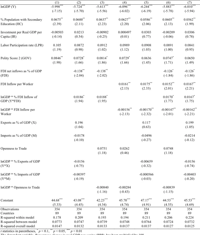
measuring the common trends. Furthermore, the coefficients of the explanatory variables for Model 3 are the most significant out of the three models. Model 3 is also consistent with the theory discussed in the introduction and literature review. The regression equation in column 2 from table 3 is used as the benchmark. Henceforth, in discussing the results of the key estimates, the coefficients of this regression equation are used. The results may slightly vary when moving from column to column. The results of the regression analysis of Model 3 are discussed below.
Dependent variable: Percentage change in real GDP per capita (PPP)
(1) (2) (3) (4) (5) (6) (7)
lnGDP (Y) -5.998*** -5.724*** -5.613*** -6.096*** -6.244*** -5.883*** -6.010***
(-7.15) (-5.70) (-5.56) (-6.02) (-6.19) (-5.78) (-5.94)
% Population with Secondary 0.0675** 0.0600** 0.0637** 0.0627** 0.0586** 0.0605** 0.0562**
Education (HC) (2.39) (2.11) (2.23) (2.20) (2.06) (2.13) (1.99)
Investment per Real GDP per -0.00503 0.0213 -0.00902 0.000497 0.0303 -0.00209 0.0306 Capita (IR) (-0.14) (0.54) (-0.25) (0.01) (0.77) (-0.06) (0.78)
Labor Participation rate (LPR) 0.105 0.0872 0.0912 0.0989 0.0908 0.0891 0.0841
(1.19) (0.98) (1.02) (1.12) (1.03) (1.00) (0.95)
Polity Score 2 (GOV) 0.0846** 0.0728* 0.0814* 0.0729* 0.0636 0.0747* 0.0650
(1.98) (1.66) (1.86) (1.66) (1.45) (1.71) (1.49)
FDI net inflows as % of GDP -0.138** -0.138** -0.126* -0.126*
(FDI) (-2.04) (-2.02) (-1.84) (-1.86)
FDI Inflow per Worker 0.0161** 0.0175** 0.0152** 0.0167**
(2.13) (2.33) (2.01) (2.21)
lnGDP * % FDI Inflow of 0.0186* 0.0188* 0.0170* 0.0167*
GDP (Y*FDI) (1.94) (1.95) (1.77) (1.75)
lnGDP * FDI Inflow per -0.00156** -0.00170** -0.00147** -0.00162**
Worker (-2.13) (-2.32) (-2.01) (-2.21) Exports as % of GDP (X) 0.196 0.117 0.199 (1.04) (0.63) (1.05) Imports as % of GDP (M) -0.0178 -0.0496 -0.0214 (-0.10) (-0.27) (-0.12) Openness to Trade 0.0751 0.0262 0.0748 (1.18) (0.46) (1.18) lnGDP * % Exports of GDP -0.0156 -0.00659 -0.0156 (Y*X) (-0.75) (-0.32) (-0.74) lnGDP * % Imports of GDP -0.00397 -0.000566 -0.00403 (Y*M) (-0.19) (-0.03) (-0.20) lnGDP * Openness to Trade -0.00840 -0.00284 -0.00839 (-1.16) (-0.43) (-1.15) Constant 44.68*** 43.08*** 42.23*** 45.70*** 47.17*** 44.53*** 45.53*** (5.33) (4.45) (4.34) (4.74) (4.91) (4.55) (4.69) Observations 354 354 354 354 354 354 354 Countries 89 89 89 89 89 89 89
R-squared within model 0.178 0.209 0.193 0.194 0.211 0.206 0.224 R-squared between model 0.0773 0.0747 0.0739 0.0748 0.0764 0.0724 0.0732 R-squared overall model 0.0147 0.0132 0.0133 0.0137 0.0137 0.0127 0.0125 t statistics in parentheses, * p < 0.1, ** p < 0.05, *** p < 0.01
The dependent variable, Percentage change in real GDP per capita (PPP), has been multiplied by 100.
Conditional Convergence
An inverse relationship exists between the initial income level and the growth in real GDP per capita (PPP). From regression equation described in column 1, for a one unit increase in the initial GDP level, there is a 0.05998% decrease in the growth rate of real GDP per capita (PPP), controlling for other factors in the model. This result confirms the evidence of
conditional convergence. Based on this study’s results, a country with a lower initial income level experiences a greater increase in growth of real GDP per capita. This study validates Barro and Sala-i-Martin’s (1995) finding and confirms the presence of conditional
convergence.
Trade and FDI, and interaction variables between trade, FDI, and initial income level are included in the model to determine the influence of trade and FDI on the speed of conditional convergence. Since interaction terms are involved, derivatives are used to test for the
influence of trade and FDI on the speed of conditional convergence towards steady state. In the example below, the results of the column 4 and the model without trade and FDI are discussed.
Since trade is not a significant determinant in this study, the derivative of growth in real GDP per capita (PPP) with respect to lnGDP in the presence FDI is calculated. The growth rate in real GDP per capita is shown as a percentage, therefore in discussing the results for
conditional convergence and half life, the coefficients will be divided by 100.
∆ ,
, ∆ ,
0.06096 0.0000156 ,
When the mean of FDI net inflows per worker is included in the model, the derivate of growth in real GDP per capita (PPP) with respect to lnGDP is
∆ ,
Based on the above analysis, this study finds evidence that FDI slightly influences the speed of convergence.
Since Model 3 also focuses on conditional convergence- the ability to reduce the income gap between their current state and steady state, the half life of the countries can be calculated in order to determine how long it takes to reduce their income gap by half.
Without taking into account trade and FDI (as shown in column 1), the half life is calculated as such:
-
2
.05998 11.55
Since trade and FDI enhance the speed of conditional convergence, the half life value goes down. Using the mean level of FDI over time, the new half life to conditional convergence is calculated as such:
-
,
2
0.06096 0.0000156 1604.643 8.06
Assuming the same conditions as in the countries’ steady state, it takes on average 12 years for the countries in the sample to eliminate half of their income gap (between actual GDP and steady state GDP). FDI reduces the half life value slightly. The results of this study support Barro and Sala-i-Martin’s (2004) findings. Barro and Sala-i-Martin (2004) show that the half life of convergence- the time it takes for half of the initial gap to be eliminated- is around 14 years.
Human Capital
The coefficient on percentage of the population with secondary education is significant at a significance level of 5%. This implies that for a one percent increase in the percentage of the
0.06%, controlling for other factors in the model. The percentage of population with secondary education, therefore, plays a significant role in determining economic growth. In order to understand the impact of education level on economic growth, a comparison between India (a low income country based on the 1987 GDP) and the mean of high income countries can be used. 11% of the Indian population has at least a secondary education while the mean percentage of the population with a secondary education in high income countries is 37%. The difference in education level is 26%. Assuming that India and high income
countries have the same education level, India is expected to grow 1.56% faster. For economies to experience economic growth, the government shall focus on educating the population. This is mainly because with an educated population (human capital), economies are able to utilize the population’s expertise to bring in innovation and become more
productive. The skilled labor force is also able to utilize foreign technology. Hence, in the presence of a skilled labor force, a country benefits from FDI inflows, leading to a positive impact on the country’s economic growth. The results of this study match the findings of Bengoa and Sanchez-Robles (2003), and Borenztein et al (1998).They provide evidence that the impact and magnitude of FDI on economic growth depends on human capital and that the more educated the labor force, the greater is the growth in real GDP per capita.
Government/Institution
The regime or government system in place (captured by the variable polity IV score 2) also influences the level of an economy’s growth. The variable, polity IV score 2, is significant with a 90% confidence level. There is a strong positive relationship between government and GDP growth. However, the results cannot be explained using the marginal analysis as there is no meaning in increasing the government score by one unit. Since there is a positive
relationship between government and GDP growth, it can be concluded that a consolidated democracy is more beneficial to the economy. Consolidated democracies, along with higher quality of governance, bring about greater human capital accumulation, less political
instability, less corruption, and greater economic freedom. Levine and Carkovic (2002) explain that FDI remains significantly and positively linked with growth when controlling for inflation or
government size. Plumper and Martin (2003) find evidence that an increase in democracy tends
of economic growth in a non-linear manner. In addition, the beneficial impact of democracy on growth holds true only for moderate degrees of political participation.
Labor force participation
The variable labor participation rate is positively related to the growth in Real GDP per capita (PPP). The coefficient of the variable labor participation rate is only marginally significant in determining economic growth. For a one percent increase in the labor force participation rate, the growth in real GDP per capita (PPP) increases by 0.0872%, controlling for other factors in the model. The study shows that the percentage of people in the labor force does not influence economic growth as much as the skills acquired by the workers (human capital). The results mirror Wijeweera et al. (2010) findings. The coefficient of labor force participation rate has the expected sign and is statistically significant at conventional levels.
Investment per real GDP per capita
The coefficient of investment per real GDP per capita is not significant in determining economic growth. Investment per real GDP per capita is positively related to the growth in Real GDP per capita (PPP)- meaning, for a one percent increase in investment per real GDP per capita, the growth in real GDP per capita (PPP) increases by 0.0213%, controlling for other factors in the model. The results are surprising as the investment level in the country is expected to bring higher growth. The results contradict previous findings of McGrattan (1998), and Bernanke, Gu¨rkaynak (2001), and Farmer and Lahiri (2006), who find a strong positive correlation between growth rates and investment ratios. An explanation for the insignificance of the coefficient of investment ratio in this study may be the uncertain robustness of the variable as a proxy for capital stock. In their study, Rao et al. (2007) mention that when the growth equation is estimated with an instrument variable method, to minimize endogeneity bias, the equation with investment ratio seems to be fragile. Therefore, it is difficult to assess the significance of the coefficient and to draw conclusions based on this result.
Foreign direct investment
Foreign direct investment is represented by FDI net inflows as percentage of GDP and FDI inflow per worker. For both trials, FDI is significant in determining the growth in real GDP per capita (PPP) at a 90% confidence level. Since interaction terms are involved, the
derivative of change in real GDP per capita with respect to FDI is calculated to test for the influence of FDI on economic growth. The benchmark model (column 2) is used as an example.
∆ ,
,
∆ ,
0.138 0.0186 ,
To determine the impact of FDI, the derivative of the log change in real GDP per capita (PPP) with respect to FDI net inflows as a proportion of GDP is taken. In this case, if high countries are able to maintain or increase the proportion of FDI to GDP, then FDI has a higher impact on the GDP of high income countries. High income countries can obviously attract more capital and the labor force can utilize the capital efficiently. Based on the results obtained, it can be concluded that the influence of FDI net inflows as a percentage of GDP on economic growth is widening the gap between low income, middle income, and high income countries. In other words, FDI net inflows account for income divergence instead of conditional income convergence. This analysis confirms Jones (1997) findings that divergence occurs at the bottom of the income distribution ladder.
The graph below depicts the relationship between the log of real GDP per capita (in US$) and FDI net inflows as a percentage of GDP. The higher the log of real GDP per capita (the higher the level of income), the greater is the impact of FDI net inflows on the log of real GDP per capita.