Kena Fox-Dobbs a,b,, Jennifer A. Leonard a,c, Paul L. Koch b

(1)

Pleistocene megafauna from eastern Beringia: Paleoecological and

paleoenvironmental interpretations of stable carbon and nitrogen

isotope and radiocarbon records

Kena Fox-Dobbs

a,b,

⁎

, Jennifer A. Leonard

a,c

, Paul L. Koch

b a

Genetics Program/Department of Vertebrate Zoology, National Museum of Natural History, Smithsonian Institution, Washington, DC, USA b

Department of Earth and Planetary Sciences, University of California Santa Cruz, 1156 High Street, Santa Cruz, CA 95064, USA c

Department of Evolutionary Biology, Uppsala University, 75236 Uppsala, Sweden

Received 2 October 2007; received in revised form 18 December 2007; accepted 23 December 2007

Abstract

Late Pleistocene eastern Beringia is a model paleo-ecosystem for the study of potential and realized species interactions within a diverse mammalian fauna. Beringian paleontological records store a wealth of information that can be used to investigate how predator–prey and competitive interactions among consumers shifted in response to past episodes of environmental change. Two such recent periods of rapid climate change are the Last Glacial Maximum (LGM) and the end of glacial conditions at the beginning of the Holocene. Here we assemble carbon and nitrogen stable isotope, and AMS14C data collected from bone collagen of late Pleistocene carnivores and megafaunal prey species from the interior of eastern Beringia (Alaska), and reconstruct the diets of ancient Alaskan carnivores and herbivores. We are able to account for the relative influences of diet versus changing environmental conditions on variances in consumer isotope values, to identify species hiatuses in the fossil record, and to draw conclusions about paleoenvironmental conditions from faunal chronologies.

Our isotopic results suggest that there was dietary niche overlap among some Beringian herbivore species, and partitioning among other species. We rely uponδ13_{C and}_δ15_{N values of modern Alaskan C}

3plant types to infer Beringian herbivore dietary niches. Horse, bison, yak, and

mammoth primarily consumed grasses, sedges, and herbaceous plant species. Caribou and woodland muskox focused upon tundra plants, including lichen, fungi, and mosses. The network of Beringian carnivore interaction was complex and dynamic; some species (wolves) persisted for long periods of time, while others were only present during specific timeframes (large felids and ursids). Beringian carnivore diets included all measured herbivore species, although mammoth and muskox only appeared in carnivore diets during specific times in the late Pleistocene. We identified the potential presence of unmeasured diet sources that may have included forest-dwelling cervids and/or plant materials. None of the large-bodied carnivore species we analyzed (except short-faced bear) were specialized predators of a single prey species during the late Pleistocene. Differences in carnivore diet and dietary breadth between time periods either reflect changes in the relative abundances of prey on the Beringian landscape, or changes in competitive interactions among Beringian carnivore species.

Keywords:Paleoecology; Carnivore guild; Paleodietary reconstruction;Panthera atrox;Canis lupus;Homotherium;Equus lambei

1. Introduction

Twenty thousand years ago Beringia was a vast open eco-system that extended from the Yukon in North America, across

the Bering Straight and through Siberia in Eurasia (Fig. 1). For much of the late Pleistocene Beringia hosted a productive mosaic of steppe, tundra, and shrub vegetation, and a diverse fauna of large-bodied mammals (Guthrie, 2001; Zazula et al., 2003). This ancient Beringian ecosystem was not analogous to any high-latitude ecosystems present on Earth today. Dynamic changes within the Beringian ecosystem over the past 50,000 yrs were largely driven by glacial–interglacial scale climate fluctuations, and biogeographic communication between continents via the

Palaeogeography, Palaeoclimatology, Palaeoecology 261 (2008) 30–46

www.elsevier.com/locate/palaeo

⁎ Corresponding author. Department of Earth and Planetary Sciences, University of California Santa Cruz, 1156 High Street, Santa Cruz, CA 95064, USA. Tel.: +1 831 459 5088; fax: +1 831 459 3074.

E-mail address:kena@pmc.ucsc.edu(K. Fox-Dobbs).

(2)

Bering land bridge during the Last Glacial Maximum (LGM). The rapid reorganization of Beringian ecosystems at the end of the Pleistocene, which resulted in the establishment of modern tundra and boreal forest habitats, was associated with the extinction of most megafaunal species.

Our understanding of Beringian paleoenvironmental condi-tions and ecosystem dynamics during the late Pleistocene has blossomed in the past several years. We've gained new insight into the vegetation of eastern Beringia via studies of floral composition, isotopic and direct radiocarbon analyses of plant macrofossils (Wooller et al., 2007; Zazula et al., 2007), and analysis of spatio-temporal patterns in late Quaternary pollen data (Brubaker et al., 2005). Likewise, genetic and radiocarbon data extracted from fossils preserved in the permafrost shed light on the spatio-temporal dynamics of ancient mammal pop-ulations during the Pleistocene (e.g. Leonard et al., 2000; Shapiro et al., 2004; MacPhee et al., 2005; Guthrie, 2006; Barnes et al., 2007; Leonard et al., 2007). Yet, we still lack a detailed understanding of Beringian paleoecological connectiv-ity, including food web organization.

Here we use stable-isotope ratios and AMS 14C dates measured on ancient bone collagen to study the paleoecology of Pleistocene megafaunal carnivores and herbivores from eastern Beringia, as well as the paleoenvironment and paleocommunity in which they lived. We restrict the spatial scope of our study to only include predators and prey from the Fairbanks area, Alaska (Fig. 1). This allows us to eliminate potential isotopic variability among individuals due to spatial differences, and instead focus on interactions among animals that could have co-occurred on the Beringian landscape. Currently, there are few isotopic stud-ies of North American late Pleistocene predator–prey systems,

and our knowledge is primarily defined by data collected from the La Brea tar pits in southern California (Coltrain et al., 2004a; Fox-Dobbs et al., 2007), and several sites in Europe (Fizet et al., 1995; Bocherens et al., 1999; Bocherens and Drucker, 2003) and Siberia (Bocherens et al., 1996).

We explore Beringian megafaunal isotope data in two contexts. First, we investigate patterns inδ13C,δ15N, and14C records of megafaunal (N45 kg) carnivores [gray wolf (Canis lupus), American lion (Panthera atrox), scimitar-tooth sabercat (Homotherium serum)] and herbivores [caribou (Rangifer tarandus) and horse (Equus lambei)] from the Fairbanks area. The temporal trends within these δ13C and δ15N records illu-minate changing paleoclimatic and paleoenvironmental condi-tions before, during, and after the LGM in eastern Beringia. Over this N40,000-year time interval Beringian climate tran-sitioned from the relatively mild conditions of Marine Isotope Stage 3 [MIS3; N50,000 to 25,000 radiocarbon years before present (14C yr BP)] to cold and dry during the peak of the LGM (ca. 18,00014C yr BP), followed by rapid warming into the Holocene (for a review of Beringian paleoclimate see;

Anderson and Lozhkin, 2001; Elias, 2001; Bigelow et al., 2003; Brigham-Grette et al., 2004). Extensive stable isotope and14C datasets collected from fossil bone collagen of Pleistocene herbivores in Europe and western Beringia (Siberia) have established that glacial-scale paleoenvironmental changes are reliably recorded in the biogeochemistry of fossil bone (e.g.

Iacumin et al., 2000; Drucker et al., 2003a,b; Richards and Hedges, 2003; Stevens and Hedges, 2004). However no isotopic studies have used stable-isotope values of consumers at different trophic levels (carnivores and herbivores) to in-vestigate paleoenvironmental changes during the LGM.

Second, we combine the wolf, felid, horse, and caribou data with additionalδ13C andδ15N data collected from bison (Bison bison), yak (Bos grunniens), and woodland muskox (Symbos cavifrons). We use these data, along with previously published

δ13

C, δ15N, and 14C data for mammoth (Mammuthus primigenius), brown bear (Ursus arctos), and giant short-faced bear (Arctodus simus) to investigate species interactions among Beringian megafauna. Specifically, we examine patterns of niche partitioning and temporal overlap within the large-bodied carnivore guild. Was prey selection dependent upon size, abundance, and vulnerability of prey species, or upon inter-species interactions (e.g. resource competition, predation, terri-torial exclusion) among carnivores? We also use the herbivore

δ13

C and δ15N records to investigate habitat selection and foraging by Beringian herbivore species.Graham and Lundelius (1984) and Guthrie (1984, 2001) contend that strong niche partitioning among herbivores feeding in productive mosaic of vegetation allowed Pleistocene megafauna to simultaneously maximize available vegetation within a local area. There are no modern high-latitude faunas analogous to the ancient Beringian mammal community, thus our results provide new insight into a unique and extinct food web.

Carbon and nitrogen in collagen are derived from diet, thus theδ13C andδ15N values of consumer collagen reflect theδ13C and δ15N values of their diet (see review by Koch, 2007). Variation in plant δ13C and δ15N values among different

Fig. 1. Map showing western (Siberia) and eastern (Alaska and Yukon) Beringia. All specimens (except mammoth) in this study are from the Fairbanks area, Alaska. Dotted line designates the approximate extent of exposed land (Bering land bridge), and dashed line delineates the approximate edge of the Laurentide ice sheet, both at 18,00014_{C yr BP (redrawn from the Paleoenvironmental Atlas}

of Beringia; available online atwww.ncdc.noaa.gov/paleo/parcs/atlas/beringia/ index.html). Note both the proximity of the Fairbanks area to the continental ice sheet, and isolation from coastal regions to the South and West during the Last Glacial Maximum.

(3)

habitats and plant types (e.g. Ehleringer, 1991; Nadelhoffer et al., 1996; Handley et al., 1999; Ben-David et al., 2001; Wooller et al., 2007) allow us to distinguish among Beringian herbivores with different foraging preferences and to estimate the relative contributions of prey species to the diets of Beringian car-nivores. Isotopic analyses of ancient bone collagen are routinely used in archeological and paleoecological studies to reconstruct the diets of top consumers (humans and carnivores, respec-tively) (e.g. Bocherens et al., 2005; Fox-Dobbs et al., 2006). While fossil predator sample sizes are rarely large enough to investigate local population dynamics or long-term temporal patterns, Alaskan permafrost deposits are an exception; they are one of few Pleistocene depositional environments where both carnivore and herbivore fossil remains are abundant (Guthrie, 1968).

2. Methods

2.1. Sample collection

Fossil specimens were collected over the past century from placer mining gravel deposits within and around Fairbanks, Alaska. While the morphological and biogeochemical preserva-tion of permafrost fossils are generally excellent, they have no stratigraphic context when found in gravel deposits. The speci-mens used in this study were curated at the American Museum of Natural History, New York and the Canadian Museum of Nature, Ottawa. We sampled wolf (n= 82), lion (n= 8), scimitar cat (n= 11), horse (n= 32), caribou (n= 10), bison (n= 6), yak (n= 5), and woodland muskox (n= 10) specimens. We sampled both cranial and postcranial bones that were morphologically diagnostic to the species-level.

2.2. Sample preparation and analysis

Cortical bone samples [∼150 milligrams (mg)] were drilled from specimens with a handheld microdrill, and then crushed into a coarse powder in a mortar and pestle. Collagen extraction methods followBrown et al. (1988). Samples were decalcified in 0.5 N HCl at 4 °C for 1–2 days, and then rinsed in 0.01M NaOH for 4–6 h to remove organic acid contamination. Sam-ples were gelatinized in 0.01 N HCl at 58 °C for 12 h, and the gelatin solution was then passed across a 1.5 μm glass fiber filter. The filtrate was ultrafiltered (pre-cleaned Centriprep ultrafilters;Higham et al., 2006), with retention and lyophiliza-tion of the N30 kDa fraction. Collagen preservation was as-sessed with atomic C:N ratios, and all samples were between 2.2 and 2.8, which is well within the range for viable collagen (Ambrose, 1990).

For stable isotope analyses the collagen samples (1.0 mg) were weighed into tin capsules. Carbon and nitrogen stable-isotope ratios were measured using an elemental analyzer coupled with mass spectrometers at the University of California Davis Stable Isotope Facility, and the University of California Santa Cruz Stable Isotope Laboratory. Stable-isotope composi-tions are reported using the δ notation, and are referenced to Vienna PeeDee Belemnite and air for carbon and nitrogen,

respectively. The standard deviation for replicates of a gelatin standard wasb0.3‰for carbon and nitrogen for samples run at the Davis lab, andb0.2‰for carbon and nitrogen for samples run at the Santa Cruz lab.

Ancient collagen samples analyzed for radiocarbon at the Center for Accelerator Mass Spectrometry, Lawrence Liver-more National Laboratory, were prepared with the method outlined above. Since there is no agreed upon calibration curve for datesN26,00014C yr BP (Reimer et al., 2006), we present all specimen ages as uncalibrated14C dates.

2.3. Eastern Beringian carnivore dietary reconstructions We reconstructed the diets of Beringian wolves, felids, and bears by comparing them to potential Fairbanks area mega-faunal prey species. We used published isotope values for Fairbanks area Pleistocene brown bears (n= 16) and short-faced bears (n= 4) that were also 14C dated (Matheus, 1995, 1997; Barnes et al., 2002). We excluded one Fairbanks area brown bear because the collagen analyzed was from tooth dentine, not bone, and this individual had anomalously highδ13C andδ15N values (Specimen F:AM 96612). In order to account for tem-poral differences inδ13C and δ15N values we group the dated carnivores and herbivores into three climatically relevant time periods. The groups are post-glacial (18,000 to 10,00014C yr BP), full-glacial (23,000 to 18,00014C yr BP), and pre-glacial (N50,000 to 23,00014C yr BP). The post-glacial time period is characterized by the very rapid transition towards warmer, mesic conditions of the Holocene. The full-glacial is the 5000-year period when LGM conditions were the coldest and driest (Elias, 2001; Guthrie, 2001). The pre-glacial period encom-passes mild conditions of MIS3 until∼30,00014C yr BP, and the subsequent onset of LGM cooling.

For each time period we compared carnivoreδ13C andδ15N values to those of14C dated horse and caribou individuals from the same time period, and to a range of bison, yak and woodland muskoxen δ13C and δ15N values from undated specimens, which are represented by their means and standard deviations. Due to the small sample of full-glacial caribou (n= 1), we calculated the full-glacial caribou mean and standard deviation (for carnivore dietary reconstructions) by combing the values of the full-glacial individual with those of the next older and next younger individuals (totaln= 3). We shifted carnivoreδ13C and

δ15

N values by−1.3‰and−4.6‰, respectively, to account for isotopic fractionations between consumers at different trophic levels (Fox-Dobbs et al., 2007). We also included means and standard deviations of δ13C and δ15N values for undated eastern Beringian (Alaska) mammoths (n= 5) in the dietary reconstructions (Bocherens et al., 1994).

2.4. Characterization of carnivore diets using IsoSource model results

In order to quantify the prey preferences of carnivore species from each time period we employedIsoSource 1.3.1, a multi-source stable-isotope mixing model, to estimate the relative contribution of megafaunal herbivore species (diet sources) to

(4)

carnivore diet (Phillips and Gregg, 2003). We ran the model for every individual wolf, lion, scimitar cat, brown bear, and short-faced bear, and included the averageδ13C andδ15N values of caribou and horse from the appropriate time periods as well as undated bison, mammoth, woodland muskoxen, and yak as potential diet sources. Because we used two isotope systems (n= 2), and greater thann+ 1 diet sources, there was no unique combination, or mixture, of diet sources to explain a given carnivore diet. Instead IsoSource output files reported all feasible diet source combinations in increments of 1%, as well as the mean, minimum, and maximum possible contributions of each diet source to an individual carnivore's diet. Dietary in-terpretations for some carnivores were complicated by the fact that both horse and bison had meanδ13C andδ15N values that were intermediate among the other four herbivore species. Specifically, it was impossible to distinguish between a car-nivore diet comprised of only horse or bison, or a mixture of other herbivores.

We categorized an individual carnivore as a muskox, caribou, mammoth or yak ‘specialist’ if theIsoSource model results met both of the following criteria; the mean contribution (for all feasible solutions) of any one prey to the carnivore's diet was greater than or equal to 50%, and the minimum feasible contribution of that same prey to diet was greater than or equal to 33%. Carnivores were also assigned to one of the muskox, caribou, mammoth, and yak specialist categories if their values were within one standard deviation of the mean values of a single prey. We made an exception for two short-faced bears whoseδ13C and/orδ15N values were higher than any measured diet sources, but were within two standard deviations of the mean caribou values (thus classified as caribou specialists). Carnivore individuals whose diet consisted of a range of prey (no diet source had a mean contribution greater than 50%) were classified as‘generalists’or‘horse/bison specialists’, since we could not distinguish between these two categories.

We created a sixth carnivore dietary category, which included individuals that did not meet the criteria for any of the categories described above, or whose diet we interpreted based upon a priori knowledge. This category included pre-glacial wolves, and pre- and post-pre-glacial brown bears, whose

δ13

C andδ15N values were lower than the measured herbivore values, suggesting the presence of an unmeasured diet source with relatively lowδ15N values. Theδ13C andδ15N values of modern Alaskan closed-habitat (forest) cervids are low (Szepanski et al., 1999; Ben-David et al., 2001), and we suggest that moose, deer, and/or elk may have been in the diets of pre- and post-glacial carnivores. Closed-habitat cervids track the expansion of boreal forests in post-glacial Beringia (Guthrie, 2006), and may have inhabited forested areas of Beringia during MIS3. Small mammals such as rodents and lagomorphs are another unmeasured diet source, but we do not know of any empirical evidence that shows modern small mammals have systematically lower δ15N values than co-occurring large herbivores. Alternatively, brown bears with relatively low

δ15

N values may have had more omnivorous diets that included insects, leaves, berries and seeds (Hilderbrand et al., 1996; Hobson et al., 2000). In the dietary reconstructions we assume

all carnivore individuals were hypercarnivorous (pure-meat diet), and use corresponding isotopic trophic fractionations (Fox-Dobbs et al., 2007). Interspecies differences in digestive physiology and inter-individual dietary preferences (e.g. omnivory) may cause variation in carnivore trophic fractiona-tions, but these factors are poorly characterized since bone collagen is rarely analyzed in carnivore feeding studies. Thus, variation in trophic fractionations may be a source of error in the dietary reconstructions. This sixth category also includes full-and post-glacial brown bears full-and lions that were classified as muskox specialists based upon theIsoSourcemodel results. We obtained infinite14C dates for the two dated woodland muskox individuals, suggesting that woodland muskoxen may not have been abundant in the interior of Beringia during the full- and post-glacial. Therefore, it seems unlikely that these full- and

Table 1

Summary of megafaunalδ13C andδ15N values (‰)

Taxon Time period n δ13C

mean δ13 C SD δ15 N mean δ15 N SD Gray wolf (Canis lupus) All 82 −19.3 0.6 7.8 1.1 Post-glacial 9 −19.2 0.6 8.0 0.4 Full-glacial 7 −19.2 0.5 9.8 1.4 Pre-glaciala 23 −19.3 0.5 7.2 1.3 Undated 43 −19.4 0.6 7.8 0.6 Scimitar cat (Homotherium serum) All (Pre-glacial) 11 −19.3 0.6 8.0 1.4 American lion (Panthera atrox) All 8 −19.0 0.4 7.8 0.7 Post-glacial 5 −18.8 0.2 7.5 0.8 Full-glacial 3 −19.3 0.6 8.2 0.2 Brown bear (Ursus arctos)b All 16 −19.0 0.5 6.8 1.6 Post-glacial 8 −18.7 0.4 7.0 1.3 Full-glacial 2 −19.1 0.2 8.2 3.0 Pre-glaciala 6 −19.5 0.4 6.1 1.5 Short-faced bear (Arctodus simus)b All 4 −18.0 0.2 8.4 0.8 Full-glacial 1 −17.8 – 8.0 – Pre-glacial 3 −18.1 0.2 8.6 0.9 Horse (Equus lambei) All 32 −21.2 0.3 3.4 1.1 Post-glacial 8 −21.0 0.2 3.5 1.1 Full-glacial 14 −21.2 0.3 4.0 0.7 Pre-glaciala 10 −21.2 0.4 2.7 1.2 Caribou (Rangifer tarandus) All 10 −19.5 0.4 3.3 1.2 Post-glacial 4 −19.4 0.5 3.5 1.4 Full-glacial 1 −20.1 – 3.6 – Pre-glaciala ₅ ₋_19.4 _0.2 _3.1 _1.2

Bison (Bison bison) Undated 6 −20.5 0.6 4.3 0.9 Yak (Bos grunniens) Undated 5 −21.6 1.5 3.2 2.7 Woodland muskox (Symbos cavifrons) Undated 10 −20.0 0.9 1.2 1.7 Mammoth (Mammuthus primigenius)c Undated 5 −21.1 0.2 7.4 1.0 Post-glacial: 18,000–10,00014_{C yr BP, Full-glacial: 23,000}_–_18,00014_{C yr BP,} Pre-glacial:N50,000–23,00014_{C yr BP.}

a _{Pre-glacial time period includes individuals with infinite}14_{C dates.} b _{Fairbanks area short-faced and brown bear data reported in}_{Matheus (1995)}

andBarnes et al. (2002).

c

(5)

Table 2

Eastern Beringian carnivore specimen ID's,δ13C andδ15N values (‰), and14C dates

Genus Dated Beringian carnivores Time group Undated Beringian wolves (Canis lupus)

Specimen ID δ13_C _δ15_N _{at. C:N} 14_{C yr BP} 14_{C Lab ID} _{Specimen ID} _δ13_C _δ15_N _{at. C:N} Canis AMNH F:AM 30450 −19.4 5.6 2.2 7751 ± 64 AA48695 Holocene AMNH 42416 −19.8 6.6 2.3

Canis AMNH F:AM 67165 −19.2 8.6 2.2 12,600 ± 150 AA42317 Post-glacial AMNH 42417 −18.9 6.8 2.3

Canis AMNH F:AM 67157 −18.7 7.9 2.3 14,690 ± 190 AA42315 Post-glacial AMNH 42418 −19.0 7.8 2.3

Canis AMNH F:AM 70944 −19.2 7.3 2.7 15,268 ± 169 AA38449 Post-glacial AMNH F:AM 142415 −19.1 6.5 2.3

Canis AMNH F:AM 30451 −18.6 8.8 2.4 15,800 ± 90 UCR3761 Post-glacial AMNH F:AM 30454 −18.3 6.8 2.3

Canis AMNH F:AM 68009-A −18.9 8.0 2.8 16,800 ± 210 AA35227 Post-glacial AMNH F:AM 30477 −19.3 8.2 2.3

Canis AMNH F:AM 30453 −18.3 9.3 2.4 19,210 ± 260 AA48702 Full-glacial AMNH F:AM 67158 −18.7 7.9 2.3

Canis AMNH F:AM 70942 −19.8 9.3 2.3 20,150 ± 110 CAMS115775 Full-glacial AMNH F:AM 67164 −19.5 7.9 2.3

Canis AMNH F:AM 67169 −19.3 10.3 2.3 20,305 ± 385 AA35216A Full-glacial AMNH F:AM 67166 −20.2 6.8 2.3

Canis CMN 9929 −19.3 12.7 2.2 20,910 ± 70 UCR3764 Full-glacial AMNH F:AM 67169 −19.2 8.1 2.3

Canis AMNH F:AM 68008-G −19.2 8.5 2.2 23,380 ± 470 AA35222 Full-glacial AMNH F:AM 67185 −19.6 8.4 2.3

Canis AMNH F:AM 67170 −18.3 7.3 2.3 27,620 ± 580 AA48694 Pre-glacial AMNH F:AM 67201 −19.5 8.3 2.3

Canis AMNH F:AM 30431 −19.1 8.6 2.3 28,500 ± 300 CAMS115776 Pre-glacial AMNH F:AM 67204 −19.3 7.4 2.2

Canis AMNH F:AM 67163 −18.8 6.6 2.4 31,800 AA48693 Pre-glacial AMNH F:AM 67209 −19.8 7.8 2.4

Canis CMN 42388 −18.5 8.5 2.6 33,900 ± 1700 AA35221 Pre-glacial AMNH F:AM 67211 −19.4 8.1 2.4

Canis AMNH F:AM 70946 −20.0 5.4 2.5 38,000 AA42313 Pre-glacial AMNH F:AM 68006-E −19.5 8.3 2.3

Canis AMNH F:AM 67243 −20.1 6.2 2.3 38,500 ± 1100 CAMS115772 Pre-glacial AMNH F:AM 68006-F −19.1 8.6 2.3

Canis CMN 17311 −19.1 6.1 2.7 38,790 ± 540 UCR3762 Pre-glacial AMNH F:AM 68006-I −18.9 8.6 2.2

Canis AMNH F:AM 67197 −20.3 5.7 2.4 39,300 ± 1230 CAMS115760 Pre-glacial AMNH F:AM 68006-J −19.5 7.4 2.3

Canis AMNH F:AM 142410 −19.4 6.2 2.3 45,400 CAMS115762 Pre-glacial AMNH F:AM 70935 −19.7 8.3 2.4

Canis AMNH F:AM 142409 −19.4 8.6 2.3 48,130 CAMS115777 Pre-glacial AMNH F:AM 70950 −19.1 8.4 2.3

Panthera AMNH F:AM 69080 −18.8 6.7 2.4 12,990 ± 70 CAMS131350 Post-glacial AMNH F:AM 70951 −19.3 7.8 2.3

Panthera AMNH F:AM 69126 −18.5 8.3 2.4 16,650 ± 110 CAMS131346 Post-glacial

Panthera AMNH 69172 −19.0 8.3 2.5 17,140 ± 110 CAMS131362 Post-glacial

Panthera AMNH F:AM 69078 −19.6 8.4 2.6 18,270 ± 130 CAMS131349 Full-glacial

Panthera AMNH 69142 −19.6 8.2 2.6 18,590 ± 130 CAMS131361 Full-glacial

Panthera AMNH 69140 −18.6 8.1 2.4 20,970 ± 180 CAMS131360 Full-glacial

Homotherium AMNH F:AM 142490 −20.7 6.6 2.4 36,200 ± 1300 CAMS131351 Pre-glacial

Homotherium AMNH F:AM 116840 −20.1 9.7 2.6 40,500 CAMS131363 Pre-glacial

Homotherium AMNH F:AM 30770i −19.2 9.2 2.5 41,900 ± 2600 CAMS131353 Pre-glacial

Ursus AMNH F:AM 95641 −18.4 4.8 na 11,940 ± 100 OxA9798 Post-glacial

(6)

post-glacial carnivores were muskox specialists, and instead may have consumed forest cervids, or had a more omnivorous diet (for brown bears only).

We do not useIsoSourceto reconstruct the diets of Beringian herbivores because few stable-isotope data have been collected from Beringian plant macrofossils. Wide ranges in modern plant

δ13

C andδ15N values would complicate dietary interpretations drawn fromIsoSource results based on modern plant isotopic data. Future isotopic analyses of Beringian plant macrofossils may allow us to explore the diets of ancient herbivores further.

3. Results

The means and standard deviations ofδ13C andδ15N values for all carnivore and herbivore species are included inTable 1, and a full list of specimens, stable-isotope data, and14C dates are presented in Tables 2 and 3. We divided the wolf, felid, bear, horse and caribouδ13C andδ15N values into post-, full-, and pre-glacial time periods. There are no differences in the means (MANOVA–F-test; pN0.05) and variances (Levene's test; pN0.05) of δ13C and δ15N values of wolf, horse and caribou with finite versus infinite14C datesN23,00014C yr BP, thus we treat all individuals with datesN23,000 14C yr BP as one group (hereafter called pre-glacial). Because most lions and scimitar cats fell into single time groups (post-glacial and pre-glacial, respectively), we did not look for temporal trends within the felid δ13C and δ15N data. Due to a small sample size we did not include the short-faced bears in the statistical analyses.

3.1. Temporal trends in Eastern Beringian megafaunal δ13C and δ15N records

We found significant differences in mean δ13C and δ15N values of wolves from the three time periods (MANOVA – Pillai's Trace Test; approximate F4,72= 5.3, p= 0.0009).

Post-hoc pairwise comparisons among groups revealed that full-glacial wolves were highly significantly different than the pre-glacial aged wolves (F-test; F2,35= 14.2, p≤0.0001), and

significantly different than post-glacial wolves (F-test; F2,35= 4.9, p= 0.013). Pre-glacial and post-glacial wolves

were not different (F-test;pN0.5). We note that the differences among wolf groups were primarily driven by differences in

δ15

N values (one-way ANOVA; F2,36= 14.1, pb0.0001),

whereas the mean δ13C values of all groups were within 0.1‰of each other (one-way ANOVA;pN0.05).Leonard et al. (2007) previously showed that there were no significant temporal differences in the variances of wolfδ13C values, but there were differences in δ15N values. In summary, we found that post-glacial wolves had significantly less variable δ15N values than wolves from the earlier time periods, and the pre-glacial wolves had the highest level of variance. The undated wolf δ13C and δ15N values were significantly different than pre-glacial (MANOVA– F-test;F2,63= 4.2,p= 0.02) and

full-glacial (MANOVA – F-test; F2,47= 20.8, pb0.0001) wolves,

but not post-glacial wolves.

There were significant differences inδ13C and δ15N values of horses from pre-glacial, full-glacial and post-glacial time periods (MANOVA –Pillai's Trace Test; approximate F4,58= Table 2 (continued)

Genus Dated Beringian carnivores Time group Undated Beringian wolves (Canis lupus)

Specimen ID δ13_C _δ15_N _{at. C:N} 14_{C yr BP} 14_{C Lab ID} _{Specimen ID} _δ13_C _δ15_N _{at. C:N} Ursus AMNH F:AM 95659 −18.5 8.0 na 13,415 ± 70 OxA9709 Post-glacial

Ursus AMNH 30422 −19.2 10.3 na 19,027 ± 132 AA17507 Full-glacial

Ursus AMNH F:AM 95671 −18.9 6.1 na 20,820 ± 120 OxA9796 Full-glacial

Ursus AMNH F:AM 95601 −20.0 3.3 na 36,137 ± 783 AA17509 Pre-glacial

Ursus AMNH F:AM 95666 −19.5 6.3 na 47,100 ± 3100 OxA9260 Pre-glacial

Ursus AMNH F:AM 95609 −19.2 7.7 na 50,800 ± 1900 OxA9767 Pre-glacial

Ursus AMNH F:AM 95640 −19.6 6.4 na 53,900 OxA9861 Pre-glacial

Arctodus AMNH F:AM 30492 −17.8 8.0 na 20,524 ± 180 AA17511 Full-glacial

Arctodus AMNH F:AM 30494 −17.8 7.7 na 25,496 ± 224 AA17512 Pre-glacial

Arctodus AMNH A-37-10 −18.3 9.5 na 27,511 ± 279 AA17513 Pre-glacial

Arctodus AMNH 99209 −18.1 8.5 na 39,565 ± 1126 AA17514 Pre-glacial na—Not available.

at. C:N—Atomic C:N.

Museum Abbreviations: AMNH—American Museum of Natural History; CMN—Canadian Museum of Nature.

14_{C Lab Abbreviations: CAMS}_—_{Center for Accelerator Mass Spectrometry, Lawrence Livermore National Lab; AA}_—_{NSF Arizona Accelerator Mass Spectrometry}

Lab UCR—Radiocarbon Lab, University of California, Riverside; OxA—Oxford Radiocarbon Accelerator Unit.

Post-glacial: 18,000–10,00014_{C yr BP, Full-glacial: 23,000}_–_18,00014_{C yr BP, Pre-glacial:}_N_50,000_–_23,00014_{C yr BP, Infinite: minimum age given.} δ13_{C and}_δ15_{N values and}14_{C dates for a subset of wolves (}_n_{= 40) are reported in}_{Leonard et al. (2007)}_.

(7)

Table 3

Eastern Beringian herbivore specimen ID's,δ13C andδ15N values (‰), and14C dates

Genus Specimen ID δ13_C _δ15_N _{at. C:N} 14_{C yr BP} 14_{C Lab ID} _{Time group}

Equus AMNH F:AM 142429 −21.28 4.29 2.4 12,310 ± 45 CAMS119982 Post-glacial

Equus AMNH F:AM 60044 −20.85 3.47 2.4 18,630 ± 100 CAMS119970 Full-glacial

Equus AMNH F:AM 60003 −21.25 1.41 2.3 24,260 ± 200 CAMS120077 Pre-glacial

Equus AMNH F:AM 60028 −20.63 4.43 2.4 48,400 CAMS120064 Pre-glacial

Rangifer AMNH F:AM 142443 −19.21 3.26 2.4 16,000 ± 190 AA48686 Post-glacial

Rangifer AMNH F:AM 142438 −20.08 3.63 2.3 21,000 ± 361 AA48680 Full-glacial

Rangifer AMNH F:AM 142446 −19.31 3.13 2.4 29,640 ± 370 CAMS120070 Pre-glacial

Rangifer AMNH F:AM 142439 −19.43 4.67 2.4 40,700 AA48681 Pre-glacial

Rangifer AMNH F:AM 142447 −19.19 1.69 2.5 45,200 CAMS120071 Pre-glacial

Bison AMNH F:AM 5092 −20.08 4.38 2.4

Bison AMNH F:AM 46555 −20.10 5.21 2.4

Bison AMNH F:AM 46858 −20.88 3.73 2.3

Bison AMNH F:AM 46856 −19.77 2.93 2.5

Bison AMNH F:AM 3135 −20.51 5.22 2.4

Bison AMNH F:AM 1636 −21.34 4.38 2.6

Bos AMNH F:AM 142448 −20.73 2.65 2.3

Bos AMNH F:AM 142449 −24.16 0.47 2.3

Bos AMNH F:AM 142450 −20.38 0.98 2.4

Bos AMNH F:AM 142451 −21.68 4.77 2.3

Bos AMNH F:AM 30657 −21.26 7.03 2.4

Symbos AMNH F:AM 142452 −20.32 0.80 2.5

Symbos AMNH F:AM 142453 −20.19 0.01 2.4

Symbos AMNH F:AM 142454 −19.96 −0.40 2.4

Symbos AMNH F:AM 142455 −19.71 −0.24 2.5

Symbos AMNH F:AM 142456 −20.94 1.16 2.4

Symbos AMNH F:AM 142457 −19.92 −0.26 2.4

Symbos AMNH F:AM 142458 −19.89 0.09 2.4 41,200 ± 1500 CAMS120072 Pre-glacial

Symbos AMNH F:AM 142459 −20.36 3.33 2.4 48,800 CAMS120073 Pre-glacial

Symbos AMNH F:AM 142460 −20.72 3.20 2.4

Symbos AMNH F:AM 142461 −17.51 3.96 2.4

(8)

2.9,p= 0.03). Post-hoc pairwise comparisons revealed full- and pre-glacial horse were different (F-test; F2,28= 5.3, p= 0.012).

Again, this difference among horse groups was largely driven by theirδ15N values (one-way ANOVA;F2,29=5.3,p= 0.011), and

not theirδ13C values (one-way ANOVA;pN0.05). Due to the limited number of full-glacial caribou and brown bears, we only tested for a difference between pre- and post-glacialδ13C and

δ15

N values for these species. We found no difference between the values of pre- and post-glacial caribou (MANOVA–F-test; pN0.05). There was a significant difference between pre- and post-glacial brown bearδ13C andδ15N values (MANOVA–F -test;F2,11= 7.8,p= 0.008), driven by a difference in theirδ13C

values (one-way ANOVA;F1,12= 15.4,p= 0.002), and not their δ15

N values (one-way ANOVA;pN0.05). The levels of variance in bear, horse and caribouδ13C andδ15N values did not change through time (Levene's test;pN0.05).

3.2. Eastern Beringian herbivoreδ13C andδ15N values Our interspecies comparison (time independent) of herbi-vore (horse, caribou, bison, yak, woodland muskoxen, mam-moth) δ13C and δ15N values found significant differences (MANOVA– Pillai's Trace Test; approximateF10, 124= 15.1, pb0.0001) among taxa. Post-hoc comparisons showed that all species were distinct (F-test;pb0.05), except for horse and yak, which had overlapping distributions ofδ13C andδ15N values. We made additional (time dependent) comparisons between the two herbivore species with abundant 14C dates (horse and caribou), although we were unable to make a full-glacial com-parison because there was only one caribou in this time period. The difference between horse and caribou persisted though the late Pleistocene; in both the pre-glacial and post-glacial time periods theirδ13C andδ15N values were different (MANOVA– F-test: Pre-glacial; F2,12= 52.0, pb0.0001 and Post-glacial; F2,9= 31.0, pb0.0001). The differences between horse and

caribou were primarily driven by theirδ13C values. 3.3. Eastern Beringian carnivoreδ13C andδ15N values

In the post-glacial there were weak interspecies differences inδ13C andδ15N values among carnivores (wolf, brown bear,

lion) (MANOVA–Pillai's Trace Test; approximateF4,38= 2.6, p= 0.05); post-hoc pairwise comparisons revealed that only wolves and brown bears were significantly different (F-test; F2,18= 6.5, p= 0.008). There were no differences among

car-nivores during the other time periods. Among carnivore species brown bears had the most variable δ13C and δ15N values in each time period. We tested for equal variances in δ13C and

δ15

N values among species from each time period, and found the only significant difference was between bear and wolfδ15N values during the post-glacial (Levene's test; F1,15= 9.3, p= 0.008).

4. Discussion

4.1. Eastern Beringian paleoenvironmental context

Eastern Beringia experienced large shifts in temperature and moisture associated with the climate fluctuations of the late Pleistocene. Beringian LGM paleoclimate was strongly affected by growth and proximity of the Laurentide ice sheet, exposure of the Bering land bridge, and a southward migration of the jet stream (Bartlein et al., 1998; Edwards et al., 2001; Elias, 2001). A range of proxy data from eastern Beringia provides evidence of these climatic changes over the past 40,000 yrs. Pollen records (Ager and Brubaker, 1985; Bigelow and Edwards, 2001), plant macrofossil assemblages (Zazula et al., 2003; Wooller et al., 2007; Zazula et al., 2007), lake sediments (Barber and Finney, 2000), ice-cores (Alley, 2000), ocean sediment cores (Phillips and Grantz, 2001), insect abundances (Elias, 2001), and mammal abundances (Guthrie, 2006) are among the physical and biotic records used to reconstruct former Beringian climate conditions. These records suggest that; 1) the interior of eastern Beringia was cold and arid during the LGM relative to pre- and post-glacial conditions, and 2) large, rapid shifts in temperature and moisture regimes were associated with the transitions into, and out of, the LGM (reviews in Elias, 2001; Guthrie, 2001; Brigham-Grette et al., 2004).

The ramifications of these climate shifts are not well un-derstood at the ecosystem-level, but fossil pollen and plant macrofossil assemblages shed light on first-order patterns of vegetation distribution and composition. In general, the milder

Table 3 (continued)

Genus Specimen ID δ13_C _δ15_N _{at. C:N} 14_{C yr BP} 14_{C Lab ID} _{Time group}

Mammuthus V-74-2a ₋_21.00 _6.40 _na Mammuthus V-78-1b ₋_21.30 _6.85 _na Mammuthus AK-170-V-1a −21.20 8.50 na Mammuthus AK-171-V-1a −21.10 8.30 na na—Not available. at. C:N—Atomic C:N.

Refer toTable 2for museum and14_{C lab abbreviations, and time group definitions.}

δ13_{C and}_δ15_{N values and}14_{C dates for all herbivore specimens are reported in}_{Leonard et al. (2007)}_.

We report14_{C dates here for two}_Symbos_specimens. Mammuthusdata reported inBocherens et al. (1994).

a _{Collagen extracted from tooth dentine.}

(9)

condition of MIS3 corresponded to the presence of both for-ested and open biomes in eastern Beringia (Anderson and Lozhkin, 2001). Forests were absent in Alaska during the LGM; instead vegetation was characterized by a productive ‘ steppe-tundra’biome that included grasses, herbs, shrubs, and sedges

(Anderson et al., 1989; Edwards and Barker, 1994; Walker et al., 2001). Beringian vegetation responded quickly to post-glacial warming and increases in precipitation, and by∼12,000

14

C yr BP the ‘steppe-tundra’ biome was fully replaced by tundra and boreal forests (Ager and Brubaker, 1985; Lozhkin

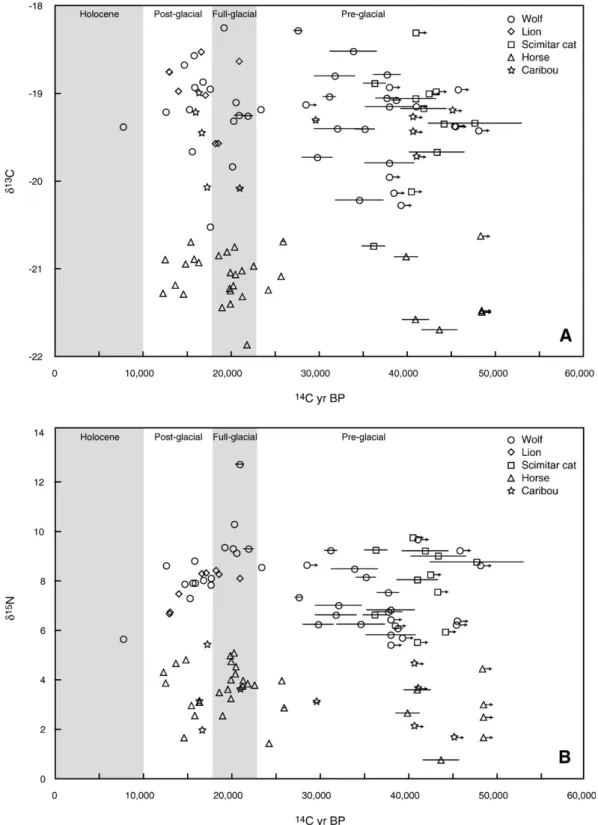
Fig. 2. Temporal records of gray wolf, lion, scimitar cat, horse and caribouδ13_{C (A), and}_δ15_{N (B) values. Records are divided into four time periods with gray shading.}

Lines through symbols indicate the error (± 1 standard deviation) associated with each14_{C date, and empty symbols indicate that the error is}_≤_{the size of the symbol.}

(10)

et al., 1993; Anderson and Brubaker, 1994; Brubaker et al., 2005).

4.2. Megafaunalδ13C records through time

The δ13C values of wolves, felids, horses, and caribou remained constant through the late Pleistocene (Fig. 2A,

Table 1). A similar pattern was observed in theδ13C values of late Pleistocene mammoth and caribou from western Beringia (Russia and Siberia) (Iacumin et al., 2000). Both the eastern and western Beringian megafaunal isotope records are sparse after 15,00014C yr BP, and end at approximately 12,50014C yr BP (Iacumin et al., 2000). Thus, the combined eastern and western Beringianδ13C datasets record neither; 1) the well-documented decrease in herbivore δ13C values that occurred after 13,500

14

C yr BP in Europe (Drucker et al., 2003b; Richards and Hedges, 2003; Hedges et al., 2004; Stevens and Hedges, 2004), and between 15,000 and 12,000 14C yr BP in southern California (Coltrain et al., 2004a), nor 2) the significant increase in theδ13C values of Fairbanks area grass macrofossils between 31,200 and 14,30014C yr BP (Wooller et al., 2007).

The decrease in megafaunal collagenδ13C values has been attributed to changes in plant δ13C values due to either a transition from an open to forested environment (e.g. canopy effect) (Drucker et al., 2003b), or plant ecophysiological response to changing atmospheric CO2concentrations (Richards

and Hedges, 2003; Stevens and Hedges, 2004; Ward et al., 2005).Stevens and Hedges (2004) compared their 40,000 yr records of horse δ13C values to δ13C records collected from wood cellulose, plant leaves, and bulk organic lake sediments and found that all showed a decrease inδ13C values at roughly the same time. Furthermore, when aligned with an ice-core derived record of CO2concentration over the same time interval

the decrease inδ13C values of organic records (herbivore, plant, lake sediment) is coeval with the increase in atmospheric CO2

concentration (Richards and Hedges, 2003; Stevens and Hedges, 2004). The paucity of latest Pleistocene (12,000 to 10,00014C yr BP) Beringian megafaunal samples precludes comparison with European megafaunalδ13C data from that time period.Wooller et al. (2007)correlated the increase in Fairbanks area grassδ13C values from 31,200 to 14,300 14C yr BP to higher aridity associated with the LGM. The pre- and full-glacial Beringian megafaunalδ13C datasets are robust, and yet do not reflect the contemporaneous rise in Beringian grassδ13C values (∼2‰). While grass tissues represent both a temporal and spatial snapshot of environmental conditions, the megafaunal bone collagenδ13C values reflect several years of an animals' diet and movement. From these results we conclude that changes in moisture availability affecting grass isotope values were very local, affected habitats that herbivores did not use, and/or did not affect all plants similarly.

4.3. Megafaunalδ15N records through time

There are two significant shifts in Beringian megafaunal bone collagenδ15N values; an increase between the pre- and full-glacial time periods, and a subsequent decrease between

full- and post-glacial time periods (Fig. 2B, Table 1). The timings of the shifts are similar in Fairbanks area horses, wolves, brown bears, and lions, but the magnitude of the shifts differs among species. The caribou, short-faced bear and scim-itar cat δ15N records are difficult to interpret because of low temporal resolution. There are several ways, and even com-binations of ways, to account for temporal patterns in consumer

δ15

N values. Changes in carnivoreδ15N values can either re-flect shifts in consumption of prey with differentδ15N values, or variation in theδ15N values of a constant diet (specific type of prey). In turn, herbivoreδ15N values record both changes in diet (e.g. grass versus shrub), and environmentally-mediated changes in theδ15N values of plants.

Our results suggest that either all species changed diets synchronously, or that portions of the shifts in the megafaunal isotope values are food web-wide and therefore climate-driven. Horses feed on a mix of grass, herbs, and shrubs (Berger, 1986; Hoppe et al., 2004), so it is possible that shifts in the consumption of different plant types could account for the observed pattern in theirδ15N values. Yet, the coeval changes in wolf, lion and bear δ15N values, none of which were horse-specialists, suggest that the δ15N values of other Beringian herbivore species also shifted, pointing to a bottom-up, climate-driven factor. The magnitude of the shift in carnivore δ15N values is greater than the shift in horse values, and likely reflects both environmental and dietary (prey selection) changes. For example, a greater reliance on mammoth versus muskox in the full- versus pre-glacial can account for the fraction of the shift in wolfδ15N values that is greater than the increase in horseδ15N values. Carnivore diets are discussed in more detail below.

If the changes, or some fraction of the changes, in mega-faunal δ15N values were environmentally-mediated, than the higher averageδ15N values during the full-glacial may reflect increased aridity in the interior of eastern Beringia during the LGM. Modern studies have identified a significant inverse correlation between δ15N values of terrestrial ecosystems and mean annual rainfall (Heaton, 1987; Handley et al., 1999; Swap et al., 2004). In each of these studies the authors found that mean annual rainfall accounted for nearly 50% of the variability in plantδ15N values. In the few modern (non-Arctic) regions where it has been tested, taxon-specific collagen nitrogen isotope values are inversely correlated with moisture-related climate variables (Heaton et al., 1986; Sealy et al., 1987; Cormie and Schwarcz, 1994; Gröcke et al., 1997). Megafaunal

δ15

N values likely also reflect changes in the types of vegetation present between interglacial and glacial periods. The occur-rences of low consumerδ15N values in the pre-glacial and post-glacial may record the presence of forest habitats, as well as generally moister conditions. The relative influences of diet and environment on megafaunalδ15N values may become clearer as additional isotopic and radiocarbon datasets are collected from Beringian fossils.

For comparison, large temporal shifts in Pleistocene European herbivoreδ15N values are neither synchronous between European regions, nor congruent with the pattern we observe in eastern Beringian fauna. Herbivores from northwestern Europe and the United Kingdom have post-glacialδ15N values that are∼5‰

(11)

lower than pre-glacial values (Richards and Hedges, 2003; Stevens and Hedges, 2004). The data from this region are sparse during the LGM, making it difficult to determine if the decrease in

δ15

N values was initiated during, or after the LGM. Post-glacial

δ15

N values remain low until 13,00014C yr BP, and then rebound to pre-glacial levels by 10,00014C yr BP (Richards and Hedges, 2003; Stevens and Hedges, 2004). A similar 15N-depletion (∼3‰) is evident in herbivore records from southwestern France (Drucker et al., 2003a).Stevens and Hedges (2004)highlight the potential effects of temperature on ecosystemδ15N values at the glacial–interglacial scale, and suggest that low post-glacialδ15N values in Europe may have persisted even as temperatures warmed due to increased moisture availability associated with permafrost melting.

4.4. Herbivore habitat use

Recent molecular and radiocarbon studies have shown that Beringian herbivore populations were not spatially or evolutio-narily static during the last 50,000 yrs of the Pleistocene (Shapiro et al., 2004; Drummond et al., 2005; MacPhee et al., 2005; Barnes et al., 2007). Of the herbivore species we analyzed for this study only caribou are present in Alaska today. Horses went extinct in the region between 12,000 and 11,00014C yr BP, coincident with a severe decrease in bison abundance, followed by the extinction of bison at approximately 900014C yr BP (Guthrie, 2006). In the ∼10,000 yrs prior to their extinction it appears that horses underwent a reduction in body size, a response in mammals that can be driven by extended resource limitation (Guthrie, 2003) or a more direct response to climatic warming. Population dynamics of other herbivore species were also changing during this interval; mammoths went extinct in interior Alaska at approximately 11,00014C yr BP, and moose appeared and elk became abundant in the fossil record between 13,000 and 12,00014C yr BP (Guthrie, 2006). However, the most important faunal change at this time in eastern Beringia may have been the arrival of humans. Un-tangling the relative impacts of climate-driven environmental change and human predation upon herbivore population sizes in the latest Pleistocene has proven difficult (Barnosky et al., 2004). In their review of current evidenceKoch and Barnosky (2006) conclude that the megafaunal extinction in eastern Beringia was likely caused by climate-driven changes to the paleoenvironment, exacerbated near the end by the arrival of

Fig. 3. Dietary reconstructions for14C dated late Pleistocene Fairbanks area gray wolves, lions, scimitar cats, brown bears, and short-faced bears from three time periods during the late Pleistocene (as inFig. 2). Brown bear and short-faced bear data are fromMatheus (1995, 1997)and Barnes et al. (2002). In each reconstruction the carnivoreδ13C andδ15N values have been corrected for trophic level isotopic fractionations (−1.3‰forδ13C and−4.6‰forδ15N; Fox-Dobbs et al., 2007), and are compared to isotope values of megafaunal prey species from the Fairbanks area (except for mammoth, which are from sites throughout Alaska;Bocherens et al., 1994). Horse and caribou individuals are

14_{C dated, and isotopic values are included for individuals from each time}

period. Bison, yak, muskox, and mammoth are not14_{C dated, and the same}

ranges of isotopic values (means ± standard deviations) are included for each time period. Dashed lines that delineate the muskox range of values in the full-and post-glacial indicate that muskoxen were included in the dietary reconstructions, but probably were not present in the Fairbanks area during these times periods. B—Bison, C—caribou, H—horse, Mm—mammoth, Mx—woodland muskox, Y—yak.

(12)

humans. They cite as evidence the lack of synchrony in the timing of extinction among megafaunal species, and the mag-nitude of ecosystem change (e.g. steppe-tundra to boreal forest) in Beringia (Koch and Barnosky, 2006). In contrast, the megafaunal extinction in North America south of the LGM ice sheets was highly synchronous among species, suggesting that humans had a larger role in the extinction (Barnosky et al., 2004).

Our isotopic results suggest that in the 30,000 yrs leading up the late Pleistocene extinction there was dietary niche overlap among some Beringian herbivore species, and partitioning among most species (Table 1,Fig. 3). We rely uponδ13C and

δ15

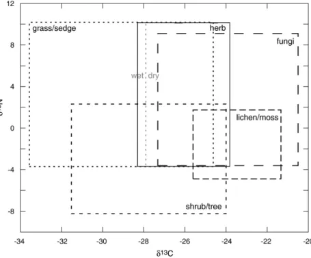
N values of modern Alaskan C3 plant types presented in

Fig. 4 to infer Beringian herbivore dietary niches. We do not directly compare the vegetation and faunal isotope values, but rather use the relative position of different plants and herbivores inδ13C and δ15N space to estimate herbivore habitat use and diet qualitatively. The range in grass and sedgeδ15N values is not wholly empirical, but instead is inferred from the range of values for herbaceous plants (herbs), and sedge values (Nadelhoffer et al., 1996). We assume that the wide range in herbδ15N values captures the potential range in grass and sedge

δ15

N values.

Theδ13C values of the Beringian herbivores are all within the range of values expected for animals feeding within an environment dominated by C3plants (Cerling et al., 1997). At

the regional scaleδ13C values vary amongst C3plants due to

ecophysiological differences, and local aridity and soil moisture conditions, with higher δ13C values correlated to higher plant water-use efficiency and drier environments (Ehleringer, 1991;

Ehleringer and Monson, 1993; Wooller et al., 2007). This has been observed in modern interior Alaskan grasses and sedges collected from wet and dry environments, and we indicate in

Fig. 4theδ13C value half-way between the dry and wet mean values (Wooller et al., 2007). Variation inδ13C values among herbivores likely reflects both the relative contribution of lichens and fungi (tundra vegetation) to diet, and the water-use efficiency of other types of vegetation.

As mentioned previously, plantδ15N values can vary due to a range of ecophysiological and environmental parameters. The variation in δ15N values between Beringian herbivores may reflect the contribution of different plant types to diet, with fungi and grasses/sedges having relatively higherδ15N values than lichens, mosses and shrubs/trees (Nadelhoffer et al., 1996; Ben-David et al., 2001). Herbivores consuming similar plant types in areas with varying soil moisture conditions may also have different δ15N values, with higher moisture levels gen-erally corresponding to lower plantδ15N values (Handley et al., 1999). Differing animal physiologies or dietary quality may also contribute to inter-individual variance in δ15N values. For example, the protein content of herbivore forage can influence the magnitude of the isotopic fractionation that occurs during the assimilation of dietary macromolecules into herbivore bone collagen (Sponheimer et al., 2003). As such, a horse feeding primarily on grass (low protein forage) may have a lower collagen δ15N value than a herbivore feeding on shrubs (high protein forage), even when the two types of vegetation have identical δ15N values. Finally, there may be taxon-specific differences among herbivores, such as the highδ15N values of mammoths (Koch, 1991; Bocherens et al., 1994; Iacumin et al.,

Fig. 4. Theoretical figure demonstrating the range ofδ13_{C and}_δ15_{N values for Beringian plant and habitat types, based upon published values for modern Alaskan}

vegetation. Boxes for each plant type encompass the means and standard deviations ofδ13_{C and}_δ15_{N values. Grass/sedge values are from}_{Wooller et al. (2007)}_and Nadelhoffer et al. (1996), herb and fungi values are fromBen-David et al. (2001), shrub/tree and lichen/moss values are fromBen-David et al. (2001)andNadelhoffer et al. (1996). See text for a description of how the grass/sedge box is defined.

(13)

2000). While the differences in δ15N values of fungi versus lichen, and plants growing in wet versus dry soils have been measured in modern ecosystems, there is no conclusive evi-dence for why mammoths consistently have higherδ15N values than contemporaneous grazing species.

Horse and yak had overlapping distributions of δ13C and

δ15

N values, indicating similar diets that 5 were potentially comprised of grasses, sedges, and herbs (Fig. 4). The exact amount of dietary overlap is difficult to determine with carbon and nitrogen isotopes alone, since C3grasses, sedges and herbs

from the same area can have identical isotopic values (Cerling et al., 1997). Modern bison are obligate grazers (Coppedge et al., 1998), and the slightly higher δ13C andδ15N values of Beringian bison compared to horse and yak during the pre- and post-glacial may correspond to pure-grass diet, versus a mixed grass and shrub/tree diet. Paleoecologic interpretations drawn from dental wear patterns and 14C records provide additional insight into Beringian herbivore habitat use. Specifically, mesowear and microwear patterns on Beringian bison and horse teeth show comparable levels of abrasion, indicative of a graminoid-rich diet for both (Solounias et al., 2004). Likewise,

Guthrie (2006)cited the disappearance of Beringian horses at 11,00014C yr BP and the subsequent abundance of bison in the radiocarbon record as potential evidence for direct competition between grazing species. Our isotopic results do not demon-strate complete dietary overlap between horse and bison, and instead suggest that Beringian bison, yak, and horse foraged on grasses, sedges, and herbs in the same open, steppe-tundra environment, but had slightly different dietary preferences.

We are able to conclude from the caribou and woodland muskoxen δ13C and δ15N data that the two species occupied separate dietary niches from each other, and from the yak/horse/ bison niche. Historic arctic caribou and muskoxen (Ovibos moschatus) also have differentδ13C andδ15N values (Coltrain et al., 2004b), and modern co-existing populations of muskoxen and caribou are known to consume different plant types (Ihl and Klein, 2001). Caribou select lichens, and muskoxen select mosses and sedges. Beringian caribou have relatively highδ13C and δ15N values, and using Fig. 4 as a guide, we infer that caribou diet was lichen/moss- and fungi-rich. Woodland muskoxen also have relatively high δ13C values, but unlike caribou they have very low δ15N values. We propose that ancient woodland muskoxen foraged on sedges in wetter low-land habitats, lichen-rich tundra vegetation, or some combina-tion of the two types of vegetacombina-tion. As withδ15N, the magnitude of the δ13C trophic fractionation between the proteinaceous tissues of a herbivore and its diet can vary (on the order of 0.5‰) depending upon the protein content of the plants con-sumed (protein-rich = larger fractionation;Ayliffe et al., 2004). In modern artic regions lichens are protein-poor compared to grasses, herbs and shrubs (Larter and Nagy, 2001). Variation in trophic fractionations contributes to the error associated with our interpretations of herbivore habitat use. A potential con-sequence is the difference between theδ13C values of Beringian grazers (horse/bison/yak) and tundra browsers (caribou/muskox) underestimates of the actual isotopic difference between Beringian forage types.

The relative isotopic differences among eastern Beringian horse, bison, and caribou have been observed in other Pleis-tocene locations (e.g. Iacumin et al., 2000; Drucker et al., 2003a; Richards and Hedges, 2003; Bocherens et al., 2005). Pleistocene Alaskan caribou dental mesowear and microwear patterns are similar to bison and horse, indicating a grass-rich diet (Solounias et al., 2004). The discrepancy in caribou dietary interpretations drawn from the isotopic and dental wear data may be due to the high abrasiveness of grasses relative to lichens. Even a modest amount of grass in caribou diet could account for a disproportionate fraction of dental wear. When we combine the paleodietary information gleaned from caribou isotope values and dental wear patterns we surmise that Pleistocene caribou had a mixed diet of grasses, and fungi- and lichen-rich tundra vegetation. Modern barren-ground caribou seasonally alternate between a winter diet dominated by lichen and mosses, and a summer diet of herbaceous species (Wilson and Ruff, 1999). Our study expands the geographic scope of the existing under-standing of late Pleistocene megafaunal community dynamics. The relative spacing among late Pleistocene herbivoreδ13C and

δ15

N values appears to have been remarkably conserved across continents, and through time, which implies an impressive fi-delity to dietary niche partitioning among megafaunal species. 4.5. Temporal patterns of carnivore presence and absence

Previous genetic, radiocarbon and isotopic research on Beringian wolves, brown bears, and short-faced bears illumi-nated dramatic changes within the carnivore guild during, and at the end of the late Pleistocene (Leonard et al., 2000; Barnes et al., 2002; Leonard et al., 2007). Our compilation of new and

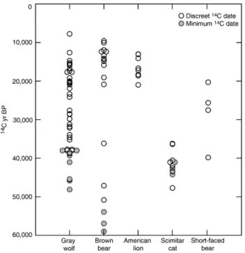
Fig. 5. Fairbanks area megafaunal carnivore ages in radiocarbon years. Open symbols represent discreet14_{C dates, and filled symbols represent minimum}14_C

dates. Brown and short-faced bear dates are fromMatheus (1997)andBarnes et al. (2002).

(14)

existing geochemical data gives further insight into how and when the members of the Beringian large-bodied carnivore guild co-existed on the landscape (Fig. 5). The temporal pat-terns of species presence and absence are compelling; of the five carnivores discussed here, we only found evidence for the persistence of gray wolves through the entire late Pleistocene. Furthermore, during most of the late Pleistocene only two or three of the five carnivore species were present, and therefore potentially interacting. Barnes et al. (2002) highlighted the staggered presence of bear species in eastern Beringia, and the different diets of brown bears that did, and did not, co-occur with short-faced bears. Felids (scimitar cats and lions) also had non-overlapping chronologies, and both were rare in the Fairbanks area during the time when short-faced bears were present (40,000 to 20,50014C yr BP). Thus, short-faced bears either dictated which carnivore species were present, or were able to persist locally while other species were absent.

Isotopic results presented below suggest that both competi-tion for resources and changing environmental condicompeti-tions could have contributed to patterns of carnivore presence/absence, although we emphasize that species interactions between an-cient animals can only be inferred, not defined, from geo-chemical records. Importantly, reconstructions of the Beringian steppe-tundra megafaunal community must be revised to reflect the dynamic patterns of predator presence and absence during the late Pleistocene.

4.6. Carnivore dietary reconstructions

Based upon our isotopic dietary reconstructions from pre-, full-, and post-glacial time periods we conclude that Beringian wolves, felids, and bears consumed a range of prey throughout the late Pleistocene. Yet when we compare dietary patterns revealed by visual assessment of the data (Fig. 3), and the IsoSourcemodel results (Fig. 6) from each time period, there are some subtle differences in prey selection. Short-faced bears were the most specialized carnivore species; all individuals were caribou specialists, including the one full-glacial indivi-dual. Except for two wolf individuals, no other carnivore species were caribou specialists in the pre-glacial. In contrast, lions, brown bears and wolves all preyed upon caribou during the full- and post-glacial. By combining isotope and presence/ absence data, we infer that short-faced bears excluded brown bears and scimitar cats from caribou in the pre-glacial.

The felids and brown bears consumed all the types of prey we analyzed. Most scimitar cats were generalists and/or horse and bison specialists, and had high dietary overlap with pre-glacial wolves. The abrupt disappearance of scimitar cats at

∼36,000 14C yr BP could be related to changing predator guild dynamics (e.g. the recent appearance of short-faced bears) and/or environmental shifts that occurred at the end of MIS3. Without data for scimitar cats from other eastern Beringian locations we cannot know if their disappearance represents a local, or regional extinction. Lions were less isotopically var-iable than the scimitar cats, and their patterns of prey preference were similar to full- and post-glacial wolves. Two post-glacial lions with low δ15N values were classified as forest cervid

specialists, which may indicate foraging in closed habitats just prior to extinction. Brown bears fall into two main categories; post-glacial caribou specialists, and individuals from all time periods that have an omnivorous diet, which included plant food sources (lower δ15N), muskox, and/or consumption of forest cervids. The one full-glacial individual classified as a mammoth specialist was most likely a scavenger, and not a mammoth predator.

Almost 50% of wolves were specialists on tundra herbivores (muskox and caribou) in the pre-glacial, whereas the other 50% were generalists and/or horse and bison specialists, or were feeding on forest cervids. In each time period wolves consumed the widest range of prey among the carnivores, matched only by lions in the post-glacial. Two full-glacial wolves were mam-moth specialists, although as with the brown bears we cannot know if this represents scavenging or predation. Mammoth did not contribute significantly to the diets of felids and short-faced bears, the only other Beringian carnivores large enough to kill a mammoth. Thus, the mammoths consumed by wolves and brown bears either died of natural causes, or were killed by one of these two carnivores. Regardless of the mechanism, it is interesting that mammoth was so rare in the diets of Beringian carnivores.

While we have established that Beringian wolves consumed a range of prey we are unable to determine with isotopes alone

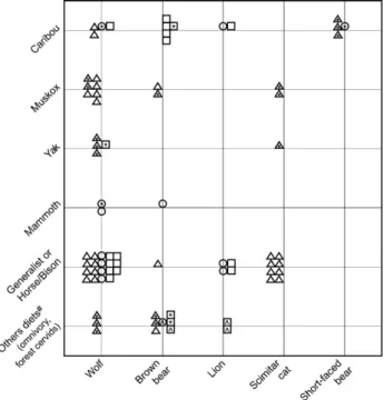
Fig. 6. Carnivore dietary categories, based upon IsoSource stable-isotope mixing model output. Symbols represent different time periods; Δ — pre-glacial, O—full-glacial,□—post-glacial. Empty symbols indicate carnivore dietary categorization derived fromIsoSourceresults, using criteria described in the text. Symbols with ⁎indicate individuals whose dietary categories were inferred from graphical assessment, because theirδ13C and/orδ15N values fell outside the dietary mixing polygon andIsoSourcecould not generate feasible diet source solutions. Symbols with ^ indicate individuals that met the criteria for muskox specialists, but were reinterpreted as omnivores and/or predators of forest cervids (moose/elk/deer). Woodland muskoxen may not have been present in the Fairbanks area in the full- and post-glacial.