A Data Mining Based Approach to Electronic Part Obsolescence Forecasting
Peter Sandborn
CALCE Electronic Products and Systems Center Department of Mechanical Engineering
University of Maryland Frank Mauro and Ron Knox PartMiner Information Systems, Inc.
Abstract – Many technologies have life cycles that are shorter than the life cycle of the product they are in. Life cycle mismatches caused by the obsolescence of technology (and particularly the obsolescence of electronic parts) results in high sustainment costs for long field life systems, e.g., avionics and military systems. This paper demonstrates the use of data mining based algorithms to augment commercial obsolescence risk databases thus improving their predictive capabilities. The method is a combination of life cycle curve forecasting and the determination of electronic part vendor-specific windows of obsolescence using data mining of historical last-order or last-ship dates. The extended methodology not only enables more accurate obsolescence forecasts but can also generate forecasts for user-specified confidence levels. The methodology has been demonstrated on both individual parts and modules.
Index Terms – Electronic parts, obsolescence, life cycle stages, data mining, flash memory, memory modules, DMSMS.
I. INTRODUCTION
A significant problem facing many “high-tech” sustainment-dominated systems is technology obsolescence, and no technology typifies the problem more than electronic part obsolescence, where electronic parts refers to integrated circuits and discrete passive components, [1,2]. The defense industry refers to electronic part obsolescence (and more generally technology obsolescence) as DMSMS – Diminishing Manufacturing Sources and Materials Shortages, [3]. In the past several decades, electronic technology has advanced rapidly causing electronic components to have shorter procurement life spans. QTEC estimates that approximately 3% of the global pool of electronic components goes obsolete every month, [4]. Driven by the consumer electronics product sector, newer and better electronic components are being introduced frequently, rendering older components obsolete. Yet, sustainment-dominated systems such as aircraft avionics are often produced for many years and maintained for decades. Sustainment-dominated products particularly suffer the consequences of electronic part obsolescence because they have no control over their electronic part supply chain due to their low production volumes. This problem is especially prevalent in avionics and military systems, where systems often encounter obsolescence problems before they are fielded and always during their support life.
Part obsolescence dates (the date on which the part is no longer procurable from its original source) are important inputs during life cycle planning for long-field life, sustaintment-dominated products, [5]. Most electronic part obsolescence forecasting is based on the development of models for the part’s life cycle. Traditional methods of life cycle forecasting utilized in commercially available tools and services are ordinal scale
based approaches, in which the life cycle stage of the part is determined from a combintation of technological attributes, e.g., [6,7] and available in commercial tools such as TACTRACTM, Total Parts Plus, and Q-StarTM. More general models based on technology trends have also appeared including a methodology based on forecasting part sales curves [8,9], and leading-indicator approaches [10]. Note, obsolescence forecasting is a form of product deletion modeling, e.g., [11], that is performed without access to internal knowledge of the manufacturer of the part.
Existing commercial forecasting tools are good at articulating the current state of a part’s availability and identifying alternatives, but are limited in their capability to forecast future obsolescence dates and do not generally provide quantitative confidence limits when predicting future obsolescence dates or risks. While a variety of electronic part obsolescence mitigation approaches exist (see [2]), they are primarily reactive in nature (applied after obsolescence occurs). Strategic obsolescence management requires more accurate forecasts, or at least forecasts with a quantifiable accuracy. Better forecasts with uncertainty estimates would open the door to the use of life cycle planning tools that could lead to more significant sustainment cost avoidance, [5,12].
This paper demonstrates the use of data mining based algorithms to augment commercial obsolescence risk databases thus increasing their predictive capabilities. The method is a combination of life cycle curve forecasting and the determination of electronic part vendor-specific windows of obsolescence using data mining of historical last-order or last-ship dates. The methodology not only enables more accurate obsolescence forecasts but can also generate forecasts for user-specified confidence levels. The methodology has been demonstrated on both individual parts and modules.
While successful electronic part obsolescence forecasting involves more than just predicting part-specific last order dates, being able to predict original vendor last order dates more accurately using a combination of market trending and data mining is an important component of an overall obsolescence risk forecasting strategy.
II. OBSOLESCENCE FORECASTING APPROACH
The obsolescence forecasting approach discussed in this paper is an extension of a previously published life cycle curve forecasting methodology based on curve fitting sales data for an electronic part [8,9]. In the existing methodology, attributes of the curve fits (e.g., mean and standard deviation for sales data fitted with a Gaussian) are plotted and trend equations are created that can be used for predicting the life cycle curve of future versions of the part type (see the next section for an example). Similar procedures could be used to forecast the life cycle trends of secondary attributes such as bias level or package type. This obsolescence forecasting approach used a fixed “window of obsolescence” determined as a fixed number of standard deviations from the peak sales year of the part. This method was evaluated along with several other approaches by Northrop Grumman (in the Air Force CPOM program) and shown to be about the same accuracy as the commercial ordinal scale forecasting approaches.
A. Example Life Cycle Curve Forecasting Algorithm – Flash Memory
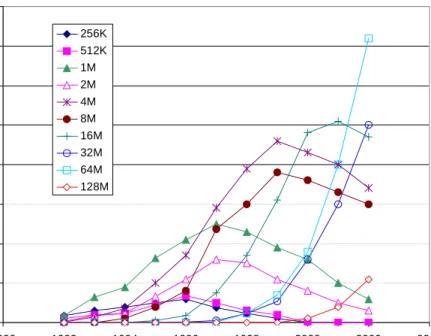
This subsection provides an example for life cycle curve forecasting for flash memory using the methodology in [8,9]. Figure 1 shows the historical and forecasted sales data for monolithic flash memory (from [13] and supplemented with more recent market
numbers). The values of μp and σp that resulted from the best Gaussian fits to the data
sets in Fig. 1 were plotted; the trends for μpand σp are shown in Figs. 2 and 3. For flash
memory the trend in peak sales year and standard deviation in number of units shipped is given by, 1997.2 ) 1.5663ln(M μp = + (1) 2.2479 M) -0.0281ln( σp = + (2)
where M is the size of the flash memory chip in megabits. The resulting trend equations, (1) and (2), can be used reproduce the life cycle curve for the parts that were used to create the relationships and for parts that are introduced in the future. For example, for M = 1 megabit, the trend equations gives μp = 1997.2 and σp = 2.25 (you can compare these
to the actual data in Fig. 1). Similarly, plugging in M = 512 megabits into (1) and (2)
0 50 100 150 200 250 300 350 400 1990 1992 1994 1996 1998 2000 2002 2004 Year N u m b e r o f U n it s S h ip p e d (M illi o n s ) 256K 512K 1M 2M 4M 8M 16M 32M 64M 128M
gives μp = 2007 and σp = 2.07 (this is a monolithic flash memory chip that was not
included in the original dataset).
When generating the life cycle curve trend equations one should be careful not to mix mil-spec parts and commercial parts. For example, (1) and (2) were generated for
y = 1.5663Ln(x) + 1997.2 1994 1996 1998 2000 2002 2004 2006 0.1 1 10 100 1000 Size (M) P e a k Sa le s Ye a r
Fig. 2. Trend equation for peak sales year (μp), for flash memory.
y = -0.0281Ln(x) + 2.2479 0 0.5 1 1.5 2 2.5 3 0.1 1 10 100 1000 Size (M) S tan d a rd D evi a ti o n ( y ea rs )
commercial flash memory chips and should only be applied to commercial flash memory chips. Mil-spec flash memory chips (if they existed) would be considered a completely different part and unique trend equations would need to be developed for them.
B. Determining the Window of Obsolescence via Data Mining
The methodology described above provides a way to create or re-create the life cycle curve for a part type given its primary attribute. Where primary attributes are attributes that can be identified with the evolution of the part over time. In the original baseline methodology, [8,9], the “window of obsolescence” specification was defined to be at 2.5σp to 3.5σp after the peak sales date (μp). In reality, the window of obsolescence
specification is not a constant but depends on numerous factors.
We suggest that the window of obsolescence specification is dependent on manufacturer-specific and part-specific business practices. For a particular part type (e.g., flash memory), historical last order date data is collected and sorted by manufacturer.1 Each part instance (data entry) in the resulting sorted data has a specific value of primary attribute (e.g., 32M) for which the peak sales date (μp) and standard
deviation (σp) can be computed using the previously created trend equations (for flash
memory these are given in (1) and (2)). The last order date for the part instance is then normalized relative to the peak sales year (i.e., the last order date is expressed as a number of standard deviations after the peak sales year). The normalization is performed for every part instance for the selected part type and manufacturer.
1 The last order date is the last date that a manufacturer will accept an order for the part. After the last order date has passed, the part is considered to be obsolete. Obsolescence of a part does not necessarily correlate to the part’s availability, i.e., some parts remain available through aftermarket sources and brokers for
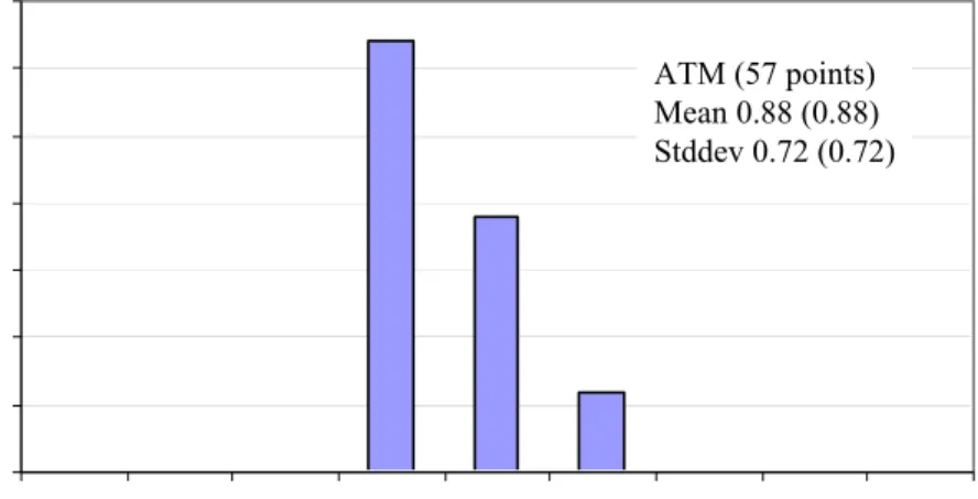
Next a histogram of the normalized vendor-specific last order dates is plotted; the histogram represents a probability distribution of when (relative to the peak sales year) the specific manufacturer obsoletes the part type. As an example, Fig. 4 shows the histogram for Atmel (ATM) flash memory (based on 57 last order dates mined from PartMiner CAPS Expert). In order to quantify the manufacturer-specific obsolescence probability, the histogram is fit with a Gaussian form and the parameters of the fit are extracted, i.e., μlo and σlo. The window of obsolescence specification is then given by,
(
μ xσ)
σp μwindow ce
Obsolescen = p + lo ± lo (3)
where x depends on the confidence level desired (i.e., x = 1 represents a 68% confidence that you have the range that accurately predicts the obsolescence event, similarly, x = 2 represents 95% confidence).
By combining the life cycle curve trends and the ATM-specific obsolescence window, the resulting obsolescence dates for ATM flash memory are given by the following equation as a function of the size in megabits (M) and confidence level desired:
0 5 10 15 20 25 30 35 -2.5 -1.5 -0.5 0.5 1.5 2.5 3.5 4.5 More Num ber of standard deviations past the peak
Nu m b e r ATM (57 points) Mean 0.88 (0.88) Stddev 0.72 (0.72)
Equation (4) assumes that the uncertainty in the window of obsolescence dominates the model uncertainty associated with the trend equations.
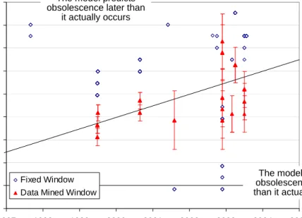
Using the methodology for the entire set of flash memory provided by PartMiner (262 data points), yields the results shown in Fig. 5. The diagonal line in the plot represents exact agreement between prediction and actual. The error bars represent a 68% confidence level. The accuracy with which the improved algorithm forecasts the obsolescence of parts is a substantial improvement over the original algorithm (“Fixed Window”).
Obsolescence date = 1.5663ln(M)+1997.2 + [0.88 ± 0.72x](-0.0281ln(M)+2.2479) Peak sales date Standard deviation
in sales data Number of standard deviations past the peak for ATM Flash
1992 1994 1996 1998 2000 2002 2004 2006 2008 2010 1997 1998 1999 2000 2001 2002 2003 2004 2005 Actual Obsolescence Date
P red ic te d O b sol e scen c e D a te Fixed Window Data Mined Window
The model predicts obsolescence later than
it actually occurs
The model predicts obsolescence earlier than it actually occurs
Fig. 5. Forecasting results for monolithic flash memory chips. 262 flash memory chips plotted. Fixed Window model = assumes a fixed window of obsolescence specification of 2.5σp to 3.5σp, Data Mined Window model = (4)
C. Application of Data Mining Determined Windows of Obsolescence to Memory Modules
As a further demonstration of the methodology described in this paper, consider its application to memory modules that are made up of multiple chips. The obsolescence of memory modules is not generally dictated by the obsolescence of the memory chips that are embedded within them. Rather, the obsolescence of memory modules is related to the beginning of availability of monolithic replacements for identical amounts of memory. As an example, in Fig. 6, the 16M DRAM module became obsolete when monolithic 16M DRAM chips became available.
In the case of DRAM memory modules, the last order date data is collected. Each module instance (data entry) has a specific value of primary attribute (e.g., 16M). For each module instance, the peak sales date (μp) and standard deviation (σp) are computed
Year 0 500 1000 1500 2000 2500 3000 92 93 94 95 96 97 98 99 00 01 02 03 04 05 U n it s s h ip pe d (i n mi ll ions )
Life cycle profile parameters:
μ= 1998.2
σ= 1.6 years
16M actual 16M forecast
Life Cycle Curve for a 16M DRAM
Monolithic 16M DRAM goes obsolete here A 16M DRAM module
might go obsolete here
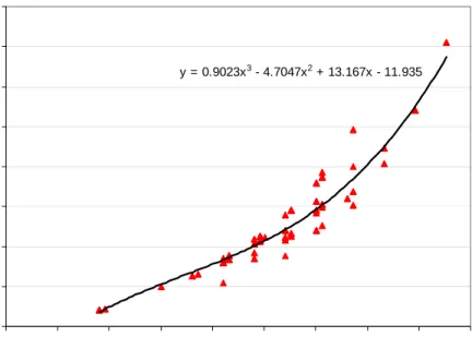
for the monolithic equivalent. The last order date for the module instance is then mapped (normalized) to the standard deviations before the peak sales date for the monolithic equivalent. In the case of memory modules, there was no need to sort the data by vendor – all the vendors considered appear to be obsoleting memory modules based on the same driver. Figure 7 shows a curve fit of the resulting data mined last order dates mapped to the life cycle curve of the monolithic equivalents.
Armed with the relation shown in Fig. 7 and the life cycle curve trends for DRAMs (e.g., see [8,9]), obsolescence dates for DRAM memory modules are given by,
In (5), x = log(M) ± α, where the value of α depends on what confidence level you want (i.e., α =0 gives you the curve fit in Fig. 7, α = 0.3 gives ~90% confidence level).
III. DISCUSSION
Successful use of existing commercial electronic part obsolescence forecasting relies on the assumption that the forecasting is updated often and that the forecasts become better (more accurate) the closer you get to the actual obsolescence date. This implies that real forecasting value depends on an organization’s ability to institute a continuous monitoring strategy and its ability to act quickly if a part accelerates toward
(5) = 1991.8M0.0011- [0.9023x3-4.7047x2+13.167x-11.935](3.1M-0.23)
Peak sales date of monolithicDRAM
Standard deviation in sales data for the monolithicDRAM Number of standard deviations before the peak of an equivalent monolithicDRAM
obsolescence.2 Unfortunately, the closer to the actual obsolescence event you get before
the forecast converges, the less useful the forecast is, and thereby the value of strategic refresh planning is limited. Being able to estimate the obsolescence date years in advance obviously provides many more options than knowing it one month in advance.
Two different types of obsolescence forecasting cases are discussed in this paper. In the first case (monolithic flash memory chips), there is not necessarily a strong correlation between the appearance of a replacement (or more technologically advanced chip) and the obsolescence of older chips, so obsolescence forecasting is based on data mining the history of how specific vendors have obsoleted parts in the past. Alternatively, for the memory modules, the forecasting algorithm leverages off the strong correlation between the appearance of a monolithic replacement for the module.
2 This implies that organizations should very carefully consider the update frequency of the electronic part
availability risk forecasting data before subscribing to a particular tool or service if they expect to make practical use of the forecasts provided.
y = 0.9023x3 - 4.7047x2 + 13.167x - 11.935 -5 0 5 10 15 20 25 30 35 0 0.5 1 1.5 2 2.5 3 3.5 4 4.5 log(size M) N u m b e r o f st a n d a rd d evi at io n s b e fo re t h e p eak
The methodology presented in this paper is a move in the direction of providing more accurate obsolescence forecasting with quantifiable confidence limits. However, the work presented in this paper does not represent a standalone solution. This approach needs to be combined with subjective information included in traditional obsolescence forecasting tools, e.g., number of sources, market share, technology factors, etc. In addition, forecasting the last order data should be combined with consolidated inventory and demand to form an effective obsolescence date for the part, e.g., [14].
It should be pointed out that the two examples presented in this paper are straightforward applications of the methodology (they are “easy” cases). Not all part types have easily identifiable primary attributes (attributes that can be identified with the evolution of the part over time), therefore, we do not claim that the methodology will be useful on every part type.
ACKNOWLEDGEMENTS
This work was funded in part by PartMiner Information Services and the National Science Foundation (Division of Design, Manufacture, and Industrial Innovation) Grant No. DMI-0438522.
REFERENCES
[1] P. Hamilton and G. Chin, “Military electronics and obsolescence part 1: The evolution of a crisis,” COTS Journal, vol. 3, no. 3, pp. 77-81, March 2001.
[2] R.C. Stogdill, "Dealing with obsolete parts," IEEE Design & Test of Computers, vol. 16, no. 2, pp.17-25, April-June 1999.
[3] H. Livingston, “GEB1: Diminishing manufacturing sources and material shortages (DMSMS) management practices,” Proceedings of the DMSMS Conference, 2000. [4] QTEC, http://www.qtec.us/Products/QStar_Introduction.htm, 2006.
[5] P. Singh and P. Sandborn, "Obsolescence driven design refresh planning for sustainment-dominated systems," The Engineering Economist, Vol. 51, No. 2, pp. 115-139, April-June 2006.
[6] A.L. Henke and S. Lai, “Automated parts obsolescence prediction.” Proceedings of the DMSMS Conference, 1997.
[7] C. Josias and J.P. Terpenny, “Component obsolescence risk assessment,” Proceedings of the 2004 Industrial Engineering Research Conference (IERC), 2004. [8] R. Solomon, P. Sandborn and M. Pecht, “Electronic part life cycle concepts and
obsolescence forecasting,” IEEE Trans. on Components and Packaging Technologies, vol. 23, no. 4, pp. 707-713, December 2000.
[9] M. Pecht, R. Solomon, P. Sandborn, C. Wilkinson, and D. Das, Life Cycle Forecasting, Mitigation Assessment and Obsolescence Strategies, CALCE EPSC Press, 2002.
[10] M. Meixell and S.D. Wu, “Scenario analysis of demand in a technology market using leading indicators,” IEEE Transactions on Semiconductor Manufacturing, vol. 14, no. 1, pp 65-78, 2001.
[11] G.J. Avlonitis, S.J. Hart and N.X. Tzokas, “An analysis of product deletion scenarios,” Journal of Product Innovation Management, Vol. 17, 2000, pp. 41-56.
[12] P. Sandborn, "Beyond reactive thinking – We should be developing pro-active approaches to obsolescence management too!," DMSMS Center of Excellence Newsletter, vol. 2, no. 3, pp. 4 and 9, July 2004.
[13] B. Matas and C. de Suberbasaux, “Chapter 5. The flash memory market,” Memory 1997, Integrated Circuit Engineering Corporation, 1997, http://smithsonianchips.si.edu/ice/cd/MEMORY97/SEC05.PDF
[14] J.R. Tilton, Obsolescence management information system (OMIS), http://www.jdmag.wpafb.af.mil/elect%20obsol%20mgt.pdf.