Road Geometry Estimation Using a Precise Clothoid Road Model and
Observations of Moving Vehicles
Maryam Fatemi, Lars Hammarstrand, Lennart Svensson, Ángel F. García-Fernández
∗ Abstract— An important part of any advanced driverassis-tance system is road geometry estimation. In this paper, we develop a Bayesian estimation algorithm using lane marking measurements received from a camera and measurements of the leading vehicles received from a radar-camera fusion system, to estimate the road up to 200 meters ahead in highway scenarios. The filtering algorithm uses a segmented clothoid-based road model. In order to use the heading of leading vehicles we need to detect if each vehicle is keeping lane or changing lane. Hence, we propose to jointly detect the motion state of the leading vehicles and estimate the road geometry using a multiple model filter. Finally the proposed algorithm is compared to an existing method using real data collected from highways. The results indicate that it provides a more accurate road estimation in some scenarios.
I. INTRODUCTION
Nowadays, active safety and autonomous driving systems provide vehicles with advanced functionalities to warn or as-sist the driver in dangerous situations. Many of the functions within these systems can benefit from accurate road geometry information. Since map data is either not accurate enough or not available for some roads, this information needs to be extracted from noisy observations provided by the on-board sensors. Two useful sources of information are measurements of the lane markings and the moving vehicles.
Road geometry estimation is a well studied subject, ex-amples of which can be found in [1], [2] and [3]. Most of these papers focus on near range road geometry estimation which is enough for some applications. However, in highway scenarios where the host vehicle has a high speed, accurate long distance information can be crucial.
Using the lane marking measurements to estimate the road has been reported in several papers including [4] and [5]. In [1], [6] and [7] the authors use the measurements of moving vehicles to update the road state. The measurements of leading vehicles can be misleading when the vehicle is changing lane/taking an exit. Therefore, in order to use these measurements correctly, one alternative is to design a mechanism that can help us distinguish between keeping lane and changing lane scenarios.
Measurements of the leading vehicles are used to jointly improve the estimation of the road geometry and host vehi-cle’s state in [1], where the algorithm only assumes that these vehicles follow their lane. Not accounting for lane changes
∗ This work was supported by VINNOVA. M. Fatemi, L.
Ham-marstrand and L. Svensson are with the department of Signals and Systems, Chalmers University of Technology, Gothenburg, Sweden. {maryam.fatemi, lars.hammarstrand, lennart.svensson}@chalmers.se. Á. F. García-Fernández is with the department of Electrical and Computer Engineering, Curtin University, Perth, Australia. [email protected].
could explain why according to the authors, their algorithm performs best when driving alone. In [6] the authors use the lateral movement of the vehicles to update the road state and they propose using a detection algorithm to distinguish between vehicles which are keeping lane and those which are not. However, according to the authors the detection algorithm suffers from a high false alarm rate. In [7], the heading of the leading vehicles is used and to avoid updating with vehicles that are changing lane/taking an exit, gating [8] is applied. In situations where we are uncertain about the road at far distances, making a hard decision about the motion state of the vehicles can lead to more sensitivity towards outliers.
In this paper we present a Bayesian inference algorithm based on a segmented clothoid-based road model that can estimate the road ahead of the host vehicle up to 200 meters. We use the shape of the lane markings and the heading of the leading vehicles to update the road state. To distinguish between keeping lane/changing lane vehicles, a multiple-model filter has been used. By following this approach we get a more robust description of our uncertainties and avoid the disadvantage of having to deal with false detections while making efficient use of the available information. Two commonly used multiple-model filters are the interacting multiple model (IMM) filter [9] [10] and the generalized pseudo-Bayesian (GPB) filter [9]. Due to computational complexity and storage considerations of the fusion system we are currently working with, GPB1 algorithm is the one that suits our purpose best. Our algorithm is evaluated on real data collected from highways across Europe. The road estimation root mean-squared error (RMSE) is used as the measure of performance.
The paper is organized as follows. We lay out the road estimation problem in Section II. The proposed road model, its resultant state parametrization and process model are explained in Section III. Section IV includes the measure-ment models. We explain our implemeasure-mentation in Section V. The evaluation of our algorithm is presented in Section VI followed by concluding remarks in Section VII.
II. PROBLEMFORMULATION ANDSYSTEMDESCRIPTION We are interested in estimating the road geometry up to 200 meters ahead of the host vehicle in highway scenarios. The road geometry is defined as the shape of the middle of the host vehicle’s lane. The road state, denotedrk, contains
that given rk, there exits a mapping1 that can describe
the road geometry in the local Cartesian coordinate system
(xlk, ylk) attached to the host vehicle. We assume that the position of the host vehicle(xhk, ykh)and its orientationψkh is known in a fixed global Cartesian coordinate system(xg, yg). In this work we consider having only one road, i.e., exits and forks are not accounted for in the designed model. Furthermore, we are working within an asynchronous fusion framework similar to the one described in [11]. This implies that the sensors are asynchronous and upon receiving the measurement of each one we align the time index of the state vector with that sensor and update with the measurement.
We aim at estimating the road geometry accurately using the measurements provided by the on-board sensors. Besides inertial measurement sensors and wheel speed sensors, our vehicle is equipped with a camera and a radar. The camera detects the left and right lane markings and describes each side by a third degree polynomial. These polynomials are given in the local coordinate system (xlk, ykl)as
ylk=l 0 k+l 1 kxlk+l 2 k(xlk) 2 +l3 k(xlk) 3 (1) ylk=r 0 k+r 1 kxlk+r 2 k(xlk) 2 +r3 k(xlk) 3 (2) where zlk = [l0 kl 1 kl 2 kl 3
k]T are the coefficients for the left
lane markings and zrk = [r0
kr 1 kr 2 kr 3
k]T for the right. These
coefficients are accompanied by two confidence values, one for each side telling us how much we can trust the coeffi-cients and up to what distance the polynomial is accurate. We use these confidence values to decide if the lane marking measurements are accurate enough to be used.
The radar detects and tracks moving objects on the road. For each observed vehicle i a measurement zi
k is reported
by the sensor given as, zik = [xi
k, yik, φik, vik]T (3)
where(xi
k, yik)is the position in the local coordinate frame
and φi
k is the heading angle relative to the heading of the
host andvi
k is the speed in that direction. It should be noted
that these values are filtered by the sensor supplier and they are not raw measurements.
The sequence of measurements up to and including timek are presented byZ1:k, the aim is to recursively calculate the
posterior density of the road staterkgiven these observations
p(rk|Z1:k).
III. ROADMODEL
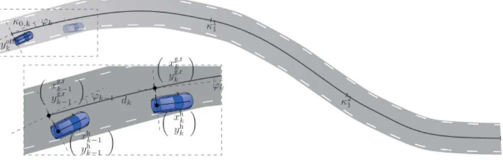
Road constructors usually follow a set of guidelines that are placed to ensure a smooth ride for the users. Among other things, this indicates that the curvature of the road can not change abruptly [12]. Based on this notion we have designed our road model. In this section we describe the clothoid-based road model, the resulting state parametrization and the process model which are illustrated in Fig. 1.
1The details of this mapping are explained in Section III-A.
A. State Parametrization
Our proposed road model consists of n connected seg-ments. Each segment is described by a clothoid, i.e., a parametric curve that has a linearly changing curvature κr(s). Therefore the curvature of segmentiis described by
κi
r(s) =κi0+κi1s (4) wheresis the arc length,κi
0 is the initial curvature and κi1 is the curvature change rate. The segments are connected to each other in a manner that ensuresG2-continuity, i.e., the position, heading and curvature of two segments are equal at their joints. Moreover, at the beginning, all the segment lengths are equal to the default segment length which isls=
lr/nwherelr denotes the road length and nis the number
of segments.
In order to describe the geometry of the road relative to the host vehicle, we need the curvature at the host vehicle’s position denoted by κ0,k and the curvature change rate
of each segment κ1
1, . . . , κn1. Furthermore, to complete our description we need the distance between the host vehicle (offset) and the starting point of the road and the heading of the road at that point denoted by ykoff and ϕk, respectively.
Note that the road parameters are expressed in the local coordinate system. Finally we can put all of these together to form the road state, which is described as
rk= [yoffk , ϕk, κ0,k, κ
1
1,k, . . . , κn1,k]T. (5)
The curvature change rates, κ1
1,k, . . . , κn1,k, are related to a
fixed part of the road andyoffk , ϕk andκ0,kare related to the
current position of the host vehicle.
A description of each segment of the road given byrk in local Cartesian coordinates is
xi r(s) = xi0+ ˆ s 0 cos(ϕi r(s))ds (6) yir(s) = yi0+ ˆ s 0 sin(ϕir(s))ds (7)
wheresdenotes the arc length into segmentiand ϕir(s) = ϕi0+κ i 0s+ κi 1 2 s 2 (8)
is the heading of segment i at that arc length. Note that xi
0, yi0, ϕi0 and κi0 are the position, heading and curvature of the starting point of segment i. Due to G2-continuity, these values are the same as the last point of the previous segment. The integrals in (6) and (7) do not have a closed form solution and we solve them by calculating the Taylor series expansion of the integrand overls/2.
B. Process Model
The parameters of the state vector describe the road ahead at each time step and as we drive along the road these parameters will change accordingly. The process model describes these changes and consists of two parts. The first part compensates for the host vehicle movement and the second part describes the evolution of the road.
The first three elements of our state vector namely ykoff, ϕk andκ0,k describe the road at the current position of the
host vehicle. So in order to calculate their time evolution we need to compensate for the movement of the host vehicle. Knowing how much we have moved along the road, we can locate the new starting point of the road and derive its offset, heading and curvature.
We receive the position and orientation of the host vehicle in a fixed global coordinate system from the fusion system. These parameters, at previous and current time stamp, are de-noted by(xhk−1, yhk−1, ψkh−1) and(xhk, yhk, ψkh), respectively.
We denote the starting position of the road at the previous time stamp by(xg,rk−1, y
g,r
k−1)and the current time stamp by
(xg,rk , yg,rk ). These coordinates are illustrated in Fig. 1. The traveled distance along the road is expressed as
dk = q (xg,rk −xg,rk−1) 2+ (yg,r k −y g,r k−1) 2. (9)
Note that (xg,rk , yg,rk ) is the intersection of two lines one originating from(xg,rk−1, y
g,r
k−1)in the direction of ϕk−1 and the other originating from(xhk, ykh)in the direction ofψhk+
π/2. Additionally, the process models of ykoff, ϕk and κ0,k
are calculated by yoffk+1 = −sin(ψhk) cos(ψkh) xg,rk −xhk ykg,r−yhk + νky ϕk+1 = ϕr(dk)−(ψkh−ψhk−1) +ν ϕ k κ0,k+1 = κr(dk) +νkκ (10)
whereκr(·)andϕr(·)are described by (4) and (8),
respec-tively. Moreover,νκ k,ν
y k andν
ϕ
k are Gaussian process noise
terms which account for the uncertainties that exist in the calculations of the host vehicle’s movement.
As stated previously, the road model consists of n seg-ments. When the host vehicle is driving within a segment, dk is subtracted from the first segment and added to the last,
additionally, the curvature change rates of all the segments remain the same.
κi
1,k+1=κi1,k ∀i= 1. . . n (11)
When the host vehicle reaches the end of the first segment, this segment is removed and a new segment is added at the end. The segment lengths are adjusted such that the road has the same total length. As the first segment is removed, the curvature rates of the remaining segments shift to the left
κi
1,k+1 =κi +1
1,k ∀i= 1. . . n−1. (12)
The curvature change rate of the new segment is calculated according to
κn
1,k=νκ
1
k (13)
where the uncertainty is modeled byνκ1
k ∼ N(0, σ
2
κ1).
IV. MEASUREMENTMODELS
We use two sets of measurements to estimate the road geometry, namely the lane marking measurements and mea-surements of the moving vehicles. Although we receive filtered tracks from the sensors, since we are not given any information about their covariances we treat them as raw measurements. In this section we describe the corresponding measurement models.
A. Lane Markings
The information about the lane markings are provided by the camera as coefficients of a third-degree polynomial. To more conveniently relate this information to the road state, we sample each polynomial by four equally spaced points up to the length where the sensor states that it is accurate. These points which completely describe the third degree polynomials, are collected in a vector calledpk.
The measurement model describes the relationship be-tween the sampled points and the state vector. The geometry of the left and right lane markings is described by translating the road half a lane width to the left and to the right. The translation is carried out by calculating the parallel clothoid of each segment similar to [5]. The following constraints are used to make sure that the translated clothoid of each segment (to either right or left), is parallel to the segment
˜ ϕ0 = ϕ0 ˜ si = si −ω L k 2 ∆ϕ i ˜ κi 0 = 1 1 κi 0 + ωL k 2 ∆ϕi = ∆ ˜ϕi (14) where∆ϕi=κi 0si+ κi1 2(s
i)2is the difference of the heading between the start and the end of segmenti. The lane width at time k is denoted by ωL
k the calculation of which is
explained in Section V-A.ϕ˜0 andϕ0 denote the heading at the beginning of the segment of the translated and original clothoid, respectively. Furthermore, s˜i, ˜κi
0 and κ˜i1 denote the segment length, the curvature at the current position of the host vehicle and the curvature change rate of segment i, respectively, of the translated clothoid. Accordingly, the measurement model is described by
pk=g(rk,sk, ωLk) +wlk(sk) (15)
whereg(·) is a nonlinear function performing the sampling and the translation described by (14). Furthermore,sk is a
vector which contains the sampling distances in arc length andwl
k ∼ N(0,Rl) describes the uncertainty around
mea-surement points.
B. Moving Vehicles
We use the heading of the moving vehicles to update the road state using the assumption that if the vehicle is following its lane, its heading and the heading of the road at the position of the vehicle should be approximately the same. Since this assumption is not always valid, e.g., when
xg,rk−1 yk−1g,r xh k−1 yh k−1 ϕk−1 xg,rk ykg,r xhk yh k ϕk dk yoff k κ0,k ϕk κ1 1 κ2 1
Fig. 1. Illustration of the road model, state parametrization and process model.
the vehicle changes lane or takes an exit, we propose two measurement models each describing these two scenarios. Assuming that vehicle i keeps its lane, its heading denoted by φi
k at position [xik, yki]T is approximately equal to the
heading of the road at that distance. This is expressed as φi
k = ϕr(s(xik, yki)) +η i,0
k (16)
wheres(·)denotes the arc length associated with the position of vehicleiandηki,0∼ N(0, σ2
η0).
For the case where the vehicle is changing lane/taking an exit, we propose to use the same model structure but with a higher noise level. This is described by
φi
k = ϕr(s(xik, yki)) +η i,1
k (17)
whereηi,k1∼ N(0, σ2
η1)and since the vehicle is not parallel to the road anymore,σ2
η1 has a large value . Based on these two noise models, we have two modes for each vehicle. One mode states that the vehicle follows its lane while the other states that it is changing lane/taking an exit. We denote the modes of a single vehicle at time k bymk ∈ {0,1} where
mk = 0states that the vehicle is following its lane.
Finally, to model how a vehicle transitions between these two modes, we use a transition probability matrix where each element represents a probability of the form Pr{mk|mk−1}. The transitional probabilities which have been calculated by the method mentioned in [13] are
Π=
0.982 0.018 0.008 0.992
At time k we get observations on nk leading vehicles. As
each of these vehicles can have two modes, we can form N = 2nk mode hypotheses. We denote theqth hypothesis at
timekby
mqk =
mq,k1, mq,k2, ..., mq,nk
k
The resulting nk-dimensional measurement model for a
given hypothesis is expressed as
φk =h(rk) +wok(mqk) (18)
where φk ∈ Rnk is a vector that includes the heading
measurements of all the vehicles at time k, h(rk) is a
linear function described according to (16) and (17) for each vehicle and wo
k(m q
k) ∼ N(0,Rq). Since we assume
the measurements to be independent, the measurement noise
covariance is a diagonal matrix denoted by Rq ∈ Rnk×nk
where each entry of the diagonal is equal to either σ2
η0 or σ2 η1 depending onm q k. V. IMPLEMENTATION
We follow a Bayesian approach to form the posterior density of the state vectorrkgiven measurements of the lane markings and the moving objects. This approach consists of two steps, prediction and measurement update. As the process model is nonlinear, we use a square root cubature Kalman filter (sqCKF) [14] to approximate the predicted density using the process model described in Section III-B. In this section we explain how we have implemented the measurement update step to form the posterior density. The pseudo-code of the complete filtering algorithm is presented in Algorithm 1.
ifThe filter has been initialized then
Prediction (see Section III-B);
ifLane marking measurements received then
Update with the lane marking measurements (see Section IV-A);
end
ifOther vehicles measurements receivedthen
Update with other vehicles (see Section IV-B);
end else
Initialize the filter (see Section VI);
end
Algorithm 1:Pseudo-code of the filtering algorithm.
A. Lane Markings
We use (15) to do the measurement update and since this model is nonlinear we use the sqCKF. The square root implementation is chosen due to its robustness. The lane width at timekin (15) is calculated as
ωL k = k X j=k−L l0 j−r 0 j L (19) wherel0 k andr 0
k are the zero order coefficients of the lane
marking polynomials on the left and right, respectively and Lis the window size over which we perform the averaging.
If a lane change is detected, before performing the update we translate the predicted road state accordingly (to the left or right) using (15). We detect a lane change by monitoring the offset measurements (l0
k,r
0
k) where a jump comparable to
a lane width indicates a lane change.
B. Moving Vehicles
In this part, we only use mature tracks, i.e. we wait a bit before we start using the leading vehicles observations to update our road estimates. The posterior density that results from such measurements, more specifically the heading of other vehicles on the road, is expressed as
p(rk|Z1:k) = N X
q=1
Pr{mqk|Z1:k}p(rk|mqk,Z1:k) (20)
As can be seen, we need to calculate a multiple-model posterior density for which there exists different approxi-mations e.g. the IMM filters [9] [10] and the GPB filters [9]. We are working within a real-time asynchronous fusion system which imposes some constraints on the choice of the multiple-model algorithm. More specifically, in order to use the IMM filters or the GPB filters with depth more than one, we need to propagate the means and covariances of all the models throughout the whole system. Therefore, to avoid the resulting storage and computational complexity demand, we choose the GPB1 algorithm where we can approximate the posterior density with a single Gaussian. Since we have used the sqCKF for lane marking measurement update, we have implemented the square root GPB1. This implementation increases the robustness of our filter.
We can see in (20) that calculating the multiple-model posterior density boils down to calculating the posterior den-sity resulting from each hypothesisp(rk|mqk,Z1:k)together
with its weight Pr{mqk|Z1:k}. Given the hypothesis and the
heading measurements, the posterior density is described by p(rk|mqk,Z1:k)∝p(rk|Z1:k−1)p(φk|mqk,rk) (21)
where the prediction density is calculated using the process model described in Section III-B and the likelihood function is explained in (18). The probability of each hypothesis is expressed as
Pr{mqk|Z1:k} ∝ p(φk|mqk,Z1:k−1)
× Pr{mqk|Z1:k−1} (22) where the first term is the distribution of the innovation
p(φk|mqk,Z1:k−1) = N(φk; ˆφk|k−1,Sq) (23)
and the second term is the predicted weight. These weights are calculated as Pr{mqk|Z1:k−1} = nk Y j=1 1 X mjk −1 =0 Pr{mq,jk |mjk−1} × Pr{mjk−1|Z1:k−1} (24)
where the first term comes from the transition probability matrixΠ which is explained in Section IV-B. To make the picture complete we need to calculate the following
Pr{mjk−1= 0|Z1:k−1} =
X
q∈H
Pr{mqk−1|Z1:k−1} Pr{mjk−1= 1|Z1:k−1} = 1−Pr{mjk−1= 0|Z1:k−1} where H is the set of all hypotheses in which we assume that thejth vehicle follows its lane.
As stated before, we approximate the multi-modal poste-rior in (20) as a single Gaussian. The first two moments of this approximated density are the estimated road state and its covariance. Note that we are working with the square root covariance rather than the covariance itself. We use the following notations to present the derivation of the estimated road state and its square root covariance
p(rk|mqk,Z1:k) = N(rk; ˆrqk|k,Pˆ q k|k) Pr{mqk|Z1:k} = ωq where Pˆq k|k ∈ R
n×n and n is the dimension of the state
vector. The estimated road state is expressed as
ˆ rk|k = N X q=1 ωqˆrqk|k.
We derive the square root covariance of the estimate by using techniques similar to the one presented in [15]. The estimated covariance of the Gaussian mixture of (20) is expressed as
ˆ Pk|k = X q ωqPˆqk|k + X q ωq(ˆrqk|k−ˆrk|k)(ˆrqk|k−ˆrk|k)T (25) By factoring Pˆq k|k = A q k|kA qT
k|k, where T denotes matrix
transpose, the square root covariance is found by performing two QR decompositions. The first decomposition gives us the square root matrix resulting from the first term in (25)
Mk =qr{[√ω1A1k|k ... √ωNANk|k]T}
whereMk ∈ Rn×n and qr{·} denotes performing the QR
decomposition and extracting the first n rows and columns of the transpose of the resultingRmatrix. Following the same notation the square root of the covariance matrix is
Ak|k =qr{ h h √ ω1∆ˆr1k|k ... √ωN∆ˆrNk|k i Mk i } where ∆ˆri
k|k = (ˆrik|k−ˆrk|k). Since we approximated the
posterior density in (20) by a single Gaussian distribution, it is completely described by its meanˆrk|k and square root covarianceAk|k.
VI. EVALUATION
In this section we evaluate the performance of our filter on real data collected from highways. We are mainly interested in calculating the road estimation error, i.e., we compare the true road sampled every 20 meters up to 200 meters to the estimated road sampled at the same distances. We use the
road estimation RMSE as the measure of performance. The true road is calculated from the host vehicle’s path in the global coordinate system and the lane marking coefficients l0
k andr
0
k. We calculate the host path by the dead-reckoning
method, i.e., using the internal sensor measurements. The precision of this method and the assumptions upon which we find this method reasonable are discussed in detail in [7].
We evaluate the performance in two different scenarios. The first, only using lane marking measurements to estimate the road and the second using measurements of both lane markings and moving vehicles. By comparing the results in the two scenarios, we show the benefit of using moving vehicle measurements. Furthermore, for the case where we use moving vehicle measurements, we compare the results of two different measurement update methods. The first is the sqCKF-GPB1 filter described in Section V-B and the second is the sqCKF-gating used in [7]. Gating is an outlier detection method where a measurement is only accepted as a valid measurement if the Mahanolobis distance between the measurement and the predicted measurement is below a threshold. The sqCKF-GPB1 and sqCKF-gating use the same state parametrization and process model. Their key difference in the measurement update is how they treat the measurements of other vehicles.
Both filters are initiated by the first measurements of the left and right lane markings. The settings for the process and measurement noise are expressed in terms of their standard deviations. Both filters use the same setting for the process noise, i.e., σyk = 0.4m, σkϕ = 0.5◦, σκ
k = 10−
5m−1, σκ1
k = 2e10−6m−
2, as well as for the measurement noise of the lane marking samples. The noise of the lane marking samples are 0.01m and 0.025m+sk/10 for the x and y
coordinates, respectively, wheresk is the sampling distance
in arc length. For the leading vehicles, the measurement noise is set to ση0 = 0.5◦ (keep lane) and σ
η1 = 3◦ (changing
lane), for the sqCKF-GPB1. These values are increased by the rate of 1◦/100m based on the longitudinal distance to the host vehicle. The sqCKF-gating algorithm usesση0 as the
measurement noise and the gate size is set to three. These values are set by reasoning and trial and error.
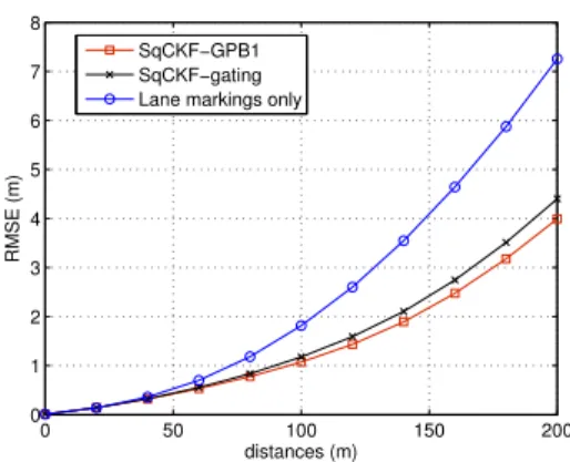
Fig. 2 compares the RMSE error of the three different cases. For this evaluation we chose a rather windy highway, the profile of which is depicted in Fig. 3, and where there were many vehicles present around the host vehicle. As can be seen, using the heading of the leading vehicles improves the performance significantly. The improvement happens for the distances over 50-60 meters and that is exactly the distances up to which we typically have lane marking mea-surements. Additionally, the sqCKF-GPB1 performs better than sqCKF-gating.
In Fig. 4 we have compared the road estimation RMSE averaged over ten log files which constitute a total of 30 minutes of driving (62.4 km). The data of these log files contain measurements recorded from different highway scenarios, i.e., windy, straight, flat and hilly highways. It should be mentioned that these log files include both busy
0 50 100 150 200 0 1 2 3 4 5 6 7 8 distances (m) RMSE (m) SqCKF−GPB1 SqCKF−gating Lane markings only
Fig. 2. Comparison of road estimation RMSE using only lane marking measurements and using both lane marking measurements and the heading of the leading vehicles. When using both measurements the sqCKF-gating and the sqCKF-GPB1 are used.
1000 2000 3000 4000 −2000 −1500 −1000 −500 0 500 1000 x axis (m) y axis (m)
Fig. 3. True road in the global coordinate system. The dots denote the position of the host vehicle on the road every 20 seconds.
0 50 100 150 200 0 0.5 1 1.5 2 2.5 3 3.5 4 4.5 5
distance along the road (m)
average RMSE (m)
lane markings only SqCKF−GPB1 SqCKF−gating
Fig. 4. Comparison of road estimation RMSE averaged over 30 minutes of driving (62.4 km).
0 20 40 60 80 100 120 140 160 180 200 0 10 20 30 40 50 60 70 80 90 100
distance along the road (m)
% Error < one lane width
sqCKF−GPB1 sqCKF−gating
Fig. 5. Percentage of the time that the road estimation RMSE is below one lane width for sqCKF-GPB1 and sqCKF-gating.
and empty highways. More specifically, in some of the log files there are many leading vehicles present while in others there are only one or two vehicles besides the host. As such, the data that has been used for evaluation includes many different real-world highway situations. The result clearly indicates that using the heading of other vehicles improves the performance significantly, additionally, the sqCKF-GPB1 filter performance is only slightly better than the sqCKF-gating algorithm. We believe the reason for this is that detecting a lane change at far distances on a rather empty and windy road is a difficult problem for both algorithms.
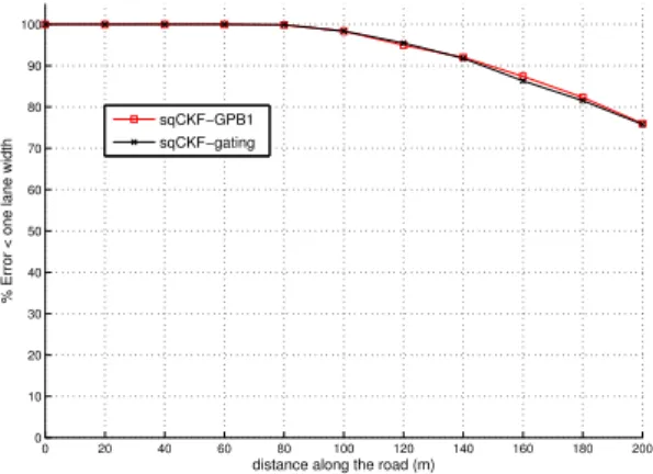
Finally, Fig. 5 depicts the percentage of the times that the road estimation RMSE is lower than one lane width for sqCKF-GPB1 and sqCKF-gating. This percentage is calculated from the same data used to generate Fig. 4. We can see that the RMSE at 200m from the host vehicle is less than one lane width 76% of the times for both algorithms.
VII. CONCLUSION
In this paper, we develop a Bayesian inference algorithm to estimate the road ahead of the host vehicle up to 200 meters, using a segmented clothoid-based road model. We use observations of the shape of the lane markings and the heading of the leading vehicles to update the road state. We use the GPB1 algorithm to distinguish between the vehicles which are keeping their lane and those that do not. We evaluate our algorithm on real data collected in highways across Europe. The results show that using the heading of leading vehicles improves the road estimation error significantly. Additionally, the sqCKF-GPB1 performs better than the sqCKF-gating in some scenarios.
Use of other sources of information such as the measure-ments of the guardrails could improve the performance of the road geometry estimation. We will address this issue in our future research.
VIII. ACKNOWLEDGMENTS
We would like to thank Volvo Car Group for providing us with the data used in the evaluations.
REFERENCES
[1] C. Lundquist and T. B. Schön, “Joint ego-motion and road geometry estimation,”Information Fusion, vol. 12, no. 4, pp. 253–263, 2011.
[2] K. Kaliyaperumal, S. Lakshmanan, and K. Kluge, “An algorithm for detecting roads and obstacles in radar images,”IEEE Transactions on Vehicular Technology, vol. 50, no. 1, pp. 170–182, Jan. 2001.
[3] Z. Zomotor and U. Franke, “Sensor fusion for improved vision based lane recognition and object tracking with range-finders,” in
Proceedings of IEEE Conference on Intelligent Transportation System, 1997, pp. 595–600.
[4] R. Chapuis, R. Aufrere, and F. Chausse, “Accurate road following and reconstruction by computer vision,”IEEE Transactions on Intelligent Transportation Systems, vol. 3, no. 4, pp. 261–270, Dec. 2002. [5] C. Gackstatter, S. Thomas, and G. Klinker, “Fusion of clothoid
segments for a more accurate and updated prediction of the road geom-etry,” inIntelligent Transportation Systems (ITSC), 13th International IEEE Conference on, Funchal, Sep. 2010, pp. 1691 – 1696.
[6] T. B. Schön, A. Eidehall, and F. Gustafsson, “Lane departure detec-tion for improved road geometry estimadetec-tion,” in Intelligent Vehicle Symposium, Tokyo, Japan, June 2006.
[7] A. F. García-Fernández, L. Hammarstrand, M. Fatemi, and L. Svens-son, “Bayesian road estimation using on-board sensors,”IEEE Trans-action on intelligent transportation systems, 2014.
[8] Y. Bar-Shalom and E. Tse, “Tracking in a cluttered environment with probabilistic data association,” Automatica, vol. 11, no. 5, pp. 451– 460, 1975.
[9] Y. Bar-Shalom and T. Fortmann, Tracking and Data Association. Academic Press, 1988.
[10] H. A. P. Blom and Y. Bar-Shalom, “The interacting multiple model algorithm for systems with markovian switching coefficients,” IEEE Transaction on Automatic Control, vol. 33, no. 8, pp. 780–783, 1988. [11] F. Bengtsson and L. Danielsson, “A design architecture for sensor data fusion systems with application to automotive safety,” in15th world congress on Intelligent Transport Systems, 2008.
[12] A. Gern, U. Franke, and P. Levi, “Robust vehicle tracking fusing radar and vision,” inInternational Conference on Multisensor Fusion and Integration for Intelligent Systems, 2001, pp. 323–328.
[13] A. K. Kristian Weiss, Nico Kaempchen, “Multiple-model tracking for the detection of lane change maneuvers,” in Intelligent Vehicles Symposium, IEEE, July 2004, pp. 937 – 942.
[14] I. Arasaratnam and S. Haykin, “Cubature Kalman filters,” IEEE Transactions on Automatic Control, vol. 54, no. 6, pp. 1254–1269, June 2009.
[15] R. van der Merwe and E. A. Wan, “The square-root unscented Kalman filter for state and parameter-estimation,” in Acoustics, Speech, and Signal Processing, IEEE International Conference on, Salt Lake City,